Chapter 4 Unified Models of Choice and Response Time
4.1 Evidence Accumulation Models
In lexical decision tasks, participants are presented with a series of words and non-words, which they must classify accordingly (i.e., by responding ‘word’ or ‘non-word’). An EAM account of this task would assume that evidence about which category each stimulus belongs to is repeatedly sampled from the environment (which potentially includes memory and the use of cognitive heuristics) until enough evidence is gathered to trigger a response.
In this example, the two possible responses are “word” or “non-word”. If the stimulus was “FOLK”, the correct response is “word”, and so we would expect evidence to be gathered at a faster rate for the “word” response (assuming that the participant knew the word) compared to the “non-word” response. For easy/familiar/highly discriminable stimuli, drift rate is high, and evidence accumulates more quickly towards the correct response. High drift rates produce fast and accurate responses. For difficult/unfamiliar/poorly discriminable stimuli, drift rate is low, and evidence accumulates more slowly towards the correct response. Low drift rates produce slow and error-prone responses.
We also estimate “non-decision time”. Non-decision time measures the extra time that occurs from “non-decision” elements, such as perceptual encoding of the stimulus, and the time taken to execute a motor response (e.g., pressing a response key). Many EAMs also include “start point” parameters, which represent where evidence starts accumulating. For example, if we have a bias towards a certain response, or prior knowledge of what the stimulus is likely to be, we may set higher start points for some decisions.
Finally, EAMs can have a variety of variability parameters (which many differ depending on the model) that control between- and within-trial variability in drift rate, and between-trial variability in start point. These parameters allows EAMs to account for the variable nature of human decisions, as even a highly practiced participant repeatedly making the same response to that same stimulus will produce a varied distribution of response times.
There are many types of evidence accumulation models, of which the commonly used models (and models used for this software) are shown in the following chapter.
4.2 Basic EAM example
In the following example, we use the Linear Ballistic Accumulator (LBA) model of decision making. This example uses no EMC2 functionality, as you can see below. A graphical description of the model is also shown. The LBA assumes a linear ballistic accumulation rate, meaning that evidence accumulates linearly, and that the accumulation process is stable over time (i.e., not subject to perturbation from within-trial noise). LBA parameters include accumulation rate v, threshold b, non-decision time t0, start point A, and accumulation rate variability sv. For this example, lets assume that we are looking at the responses from one person, for one type of simple decision, where the individual has to decide if the Gabor patch lines are tilted to the left or right.


Figure 4.1: Gabor Patches for left facing stimuli (left) and right facing stimuli (right)
4.2.1 Setup
First we load the rtdists package, which has functions for calculating the density and randomly generating data using a wide variety of EAMs.
#clear our space
rm(list=ls())

# load packages
library(rtdists)
4.2.2 Parameters
As noted above, the parameters we need to decide are: A (start point), b (threshold), t0 (non-decision time) and a v (drift rate) for each response option. Here, we assume sv = 1 for each drift rate. This follows the recommendations of Donkin et al. (Donkin et al. 2011). To generate some data using the rtdists function, we need to input some parameter values. Alternatively, we could estimate the likelihood of some parameter values given some response times and responses, but we’ll see more on that later.
4.2.2.1 Make parameters
Here we put some values into the model that we’ve come up with (these are pretty reasonable). We make the start point up to 1, t0 of 150ms (notice it is 0.15 in the model as we work on the seconds scale), we have a threshold which is added to the start point (to make sure that threshold is larger than start point, i.e., b = B + A). Drift rates are tricky, because we need one for each response. Here, we set the drift rate for response 1 (left) higher than the rate for response 2 (right) because we’re assuming this is the correct response. Let’s make some parameters and then plug them in:
A = 1               # start point
b = 1.5 + A         # threshold + start point
t0 = .15            # non-decision time
vs = list(3,1.3)    # drift rates for the two different options i.e., (response left, response right)
4.2.3 Simulation
Let’s put these values into our random generator function. One single response isn’t really informative (because of noise and variability), so here we generate 200 responses, as if a participant responded to this type of trial 200 times.
tmp <- rtdists::rLBA(n=200, A=A,b=b,t0=t0,mean_v=vs,sd_v=c(1,1),distribution="norm")
head(tmp)
## rt response
## 1 1.9608448 2
## 2 0.6539567 1
## 3 1.0933659 1
## 4 1.1582390 1
## 5 0.6360073 1
## 6 0.5741938 1Great! Now we have some data, so lets visualize this first;
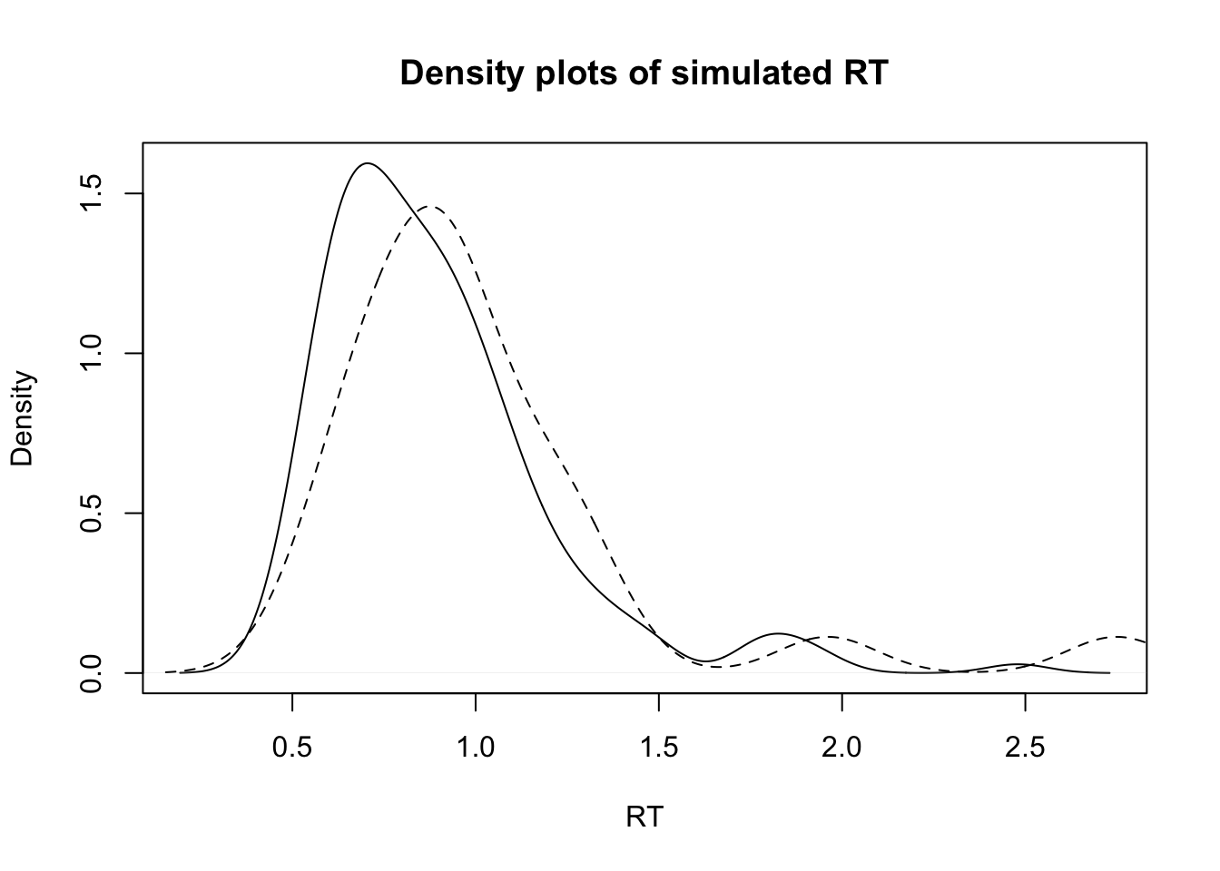
## Correct RT   Error RT
##  0.8884827  1.0234573
So we see some RT distributions and the means for correct (solid line) and incorrect (dashed line) responses. Now lets see how the likelihood works when we give it different combinations of parameters. Here we start with something bad, then something improved, and then finally the true data-generating parameters.
4.2.4 Obtain the likelihood
As mentioned above, we can also use these functions to calculate the density for model parameters, that is, the likelihood of some data given the parameter inputs. If the parameters we input to the density function are similar to that used to generate the data, then the likelihood of the parameters will be high. However, if we suggest totally wrong values, the likelihood will be low (all provided that the model actually works and recovers). This likelihood calculation is a key step in doing model estimation, which we will look at later. For now, lets see what happens if we check the likelihood given some “bad” (i.e. very different to data generating) parameters:
### Bad
A = 1
b = 0 + A
t0 = .05
vs = list(1.5,3)

ll <- rtdists::dLBA(rt=tmp$rt, response = tmp$response,A=A,b=b,t0=t0,mean_v=vs,sd_v=c(1,1))
sum(log(ll))
## [1] -1148.81Here we take the sum of the likelihood so that we can get the likelihood across all the data. You’ll notice that ll returns a vector of likelihoods. This vector has one likelihood (probability) per trial. Due to noise and variability, sometimes the “bad” parameters might seem like the right parameters. By taking the probability across all the trials, we get a more informed view (by the way, this is why we need many experimental trials to get the right parameter estimates). Now, lets see what happens when we move the parameters closer to the real ones:
### Better
A = 1
b = 0 + A
t0 = .1
vs = list(3,2)

ll <-rtdists::dLBA(rt=tmp$rt, response = tmp$response,A=A,b=b,t0=t0,mean_v=vs,sd_v=c(1,1))
sum(log(ll))
## [1] -1111.52Great! The likelihood improved (went up). It’s also worth noting here that different parameter combinations can lead to similar results (in terms or RT and responses). However, over many trials, the models can distinguish between faster drift rates and lower thresholds (generally). Finally, lets try it with the data generating parameters:
### generating

A = 1
b = 1.5 + A
t0 = .15
vs = list(3,1.5)
ll <-rtdists::dLBA(rt=tmp$rt, response = tmp$response,A=A,b=b,t0=t0,mean_v=vs,sd_v=c(1,1))
sum(log(ll))
## [1] -97.96703Again our likelihood is improved. When we do model estimation, a very similar process occurs where we continually try different parameter values until we find the most likely parameter values given the data.