Chapter 9 Advanced

9.1 Reinforcement Learning EAMs (RL-EAMs)

Data from experiment 1 of https://elifesciences.org/articles/63055 55 participants performing 52 trials on each of 4 pairs of stimuli with different levels of probabilistic reinforcement for or choosing one or other pair member.

rm(list=ls())
setwd("~/emc_advanced/")
source("emc/emc.R")
print(load("Data/mileticExp1.RData"))

## [1] "dat"

We need to first do a couple of operations on the data.

data <- dat[!dat$excl,] # Excluded participants
data$pp <- factor(as.character(data$pp))
data <- data[!is.na(data$rt),]
# Ignore presentation side, low/high reward pairs are 
# 0.6(0.8-0.2) = tT, 0.4(0.7-0.3) = eD, 0.3(.65 - 0.35) = hJ 0.2(0.6 - 0.4) = kK
# Make S factor in order of increasing ease (.2,.3,.4,.6)
data$S <- factor(paste(data$low_stim,data$high_stim,sep="_"),levels=c("k_K","h_J","e_D","t_T"))
data <- data[,c("pp","TrialNumber","S","reward","choiceIsHighP","rt")]
data$reward <- data$reward/100
names(data) <- c("subjects","trials","S","reward","R","rt")
data$R <- factor(data$R,labels=c("low","high"))
head(data)

##      subjects trials   S reward    R       rt
## 3121        7      1 e_D      1 high 0.750092
## 3122        7      2 t_T      0  low 0.866725
## 3123        7      3 e_D      0 high 1.100030
## 3124        7      4 h_J      0 high 0.708232
## 3125        7      5 k_K      1 high 1.174540
## 3126        7      6 h_J      1 high 1.483390

Looking at the data, the two lowest probability pairs not much different;

round(tapply(data$R=="high",data$S,mean),2)

##  k_K  h_J  e_D  t_T 
## 0.66 0.67 0.74 0.86

This example collapses across stimulus side, so just designates stimuli as high vs. low (reward probability).

9.1.1 Racing diffusion model with reinforcement learning

First we need to load in this particular RL model.

## [1] "dat"

source("models/RACE/RDM/rdmRL.R")

We now need to add a special component of design for adaptive models here, with only a component for adapting stimulus value, but architecture allows other components. Note that the adapt design requires reward Fcovariate and Ffunctions making one column for each stimulus (e.g., two columns for 2AFC) and corresponding columns names (p_ + stimulus name) with the probability of getting a reward.

adapt <- list( 
  stimulus=list(
    # 2AFC stimulus components whose value is to be adapted
    targets=matrix(c("K","k","J","h","D","e","T","t"),nrow=2,ncol=4,
               dimnames=list(c("high","low"),c("k_K","h_J","e_D","t_T"))),
    # adaptive equation, creating "Q" values for each stimulus component
    init_par=c("q0"),
    adapt_par=c("alpha"),
    feedback=c("reward"),
    adapt_fun=function(Qlast,adapt_par,reward) # new Q value  
      Qlast + adapt_par*(reward - Qlast),
    # Output equation, uses Q values and parameters to update rates for stimulus components
    output_par_names=c("v0","w"),
    output_name = c("v"),
    output_fun=function(output_pars,Q) # rate based on Q value
            output_pars[,1] + output_pars[,2]*Q
  ),
  fixed_pars=c("B","t0","A") # Non-adapted parameters
)


sLow <- function(d){factor(unlist(lapply(strsplit(as.character(d$S),"_"),function(x){x[[1]]})))}
sHigh <- function(d){factor(unlist(lapply(strsplit(as.character(d$S),"_"),function(x){x[[2]]})))}
pLow <- function(d){levels(d$S) <- 1-c(.6,.65,.7,.8); as.numeric(as.character(d$S))}
pHigh <- function(d){levels(d$S) <- c(.6,.65,.7,.8); as.numeric(as.character(d$S))}

matchfun <- function(d){d$lR=="high"} # "correct" (higher expected reward) response

design <- make_design(
  Ffactors=list(subjects=levels(data$subjects),S=levels(data$S)),
  Ffunctions=list(low=sLow,high=sHigh,p_low=pLow,p_high=pHigh),
  Fcovariates = c("reward"),
  Rlevels=levels(data$R),matchfun=matchfun,
  Flist=list(v0~1,v~1,B~1,A~1,t0~1,alpha~1,w~1,q0~1),
  constants = c(A=log(0),v=log(0)),
  adapt=adapt, # Special adapt component
  model=rdmRL)

##    v0     B    t0 alpha     w    q0 
##     0     0     0     0     0     0 
## attr(,"map")
## attr(,"map")$v0
##     v0
## 551  1
## 
## attr(,"map")$v
##     v
## 551 1
## 
## attr(,"map")$B
##     B
## 551 1
## 
## attr(,"map")$A
##     A
## 551 1
## 
## attr(,"map")$t0
##     t0
## 551  1
## 
## attr(,"map")$alpha
##     alpha
## 551     1
## 
## attr(,"map")$w
##     w
## 551 1
## 
## attr(,"map")$q0
##     q0
## 551  1

You will note that this is quite a few complex functions that are needed for this part, but notice that above, we only adapt some parameters (v) and keep others fixed. Further, note the alpha, q0 and w parameters that are used by the RL model.

Now we add covariates to the data (as it is used by adapt so we cannot wait until make_samplers adds it).

data <- add_Ffunctions(data,design)
head(data)

##      subjects trials   S reward    R       rt low high p_low p_high
## 3121        7      1 e_D      1 high 0.750092   e    D  0.30   0.70
## 3122        7      2 t_T      0  low 0.866725   t    T  0.20   0.80
## 3123        7      3 e_D      0 high 1.100030   e    D  0.30   0.70
## 3124        7      4 h_J      0 high 0.708232   h    J  0.35   0.65
## 3125        7      5 k_K      1 high 1.174540   k    K  0.40   0.60
## 3126        7      6 h_J      1 high 1.483390   h    J  0.35   0.65

Let’s now check that the likelihood is correct.

p_vector <- sampled_p_vector(design,doMap = FALSE)
# Average parameter table from Militic for Exp 1
p_vector["v0"] <- log(1.92) 
p_vector["B"] <- log(2.16)
p_vector["t0"] <- log(.1)
p_vector["w"] <- log(3.09)
p_vector["alpha"] <- log(0.12)
p_vector["q0"] <- log(.1) # was fixed to zero in estimated model


# All identical subjects
simdata <- make_data(p_vector,design=design,trials=52)

plot_defective_density(simdata,layout=c(2,2),factors=c("S"))

#This is slow to compute so view pdf vignettes/ReinforcementLearning/samples/profile1.pdf

Figure 9.1: RDM Likelihood

Let’s now create the model and check that the likelihood recovers using profile plots.

dadmRL <- design_model(simdata,design)
# log_likelihood_race(p_vector,dadm=dadmRL)
par(mfrow=c(2,3))
profile_pmwg(pname="v0",p=p_vector,p_min=.3,p_max=1,dadm=dadmRL)
profile_pmwg(pname="B",p=p_vector,p_min=.5,p_max=1,dadm=dadmRL)
profile_pmwg(pname="t0",p=p_vector,p_min=-3,p_max=-2,dadm=dadmRL)
profile_pmwg(pname="alpha",p=p_vector,p_min=-2.5,p_max=-1.5,dadm=dadmRL)
profile_pmwg(pname="w",p=p_vector,p_min=.75,p_max=1.5,dadm=dadmRL)
profile_pmwg(pname="q0",p=p_vector,p_min=-2.75,p_max=-2,dadm=dadmRL)

If you run these plots, you’ll see that q0 is worst estimated, in some runs down biased, in other runs up biased.

Let’s now try a larger value of q0

p_vector["q0"] <- log(1) # was fixed to zero in estimated model
simdata1 <- make_data(p_vector,design=design,trials=52)

plot_defective_density(simdata1,layout=c(2,2),factors=c("S"))

dadmRL <- design_model(simdata1,design)
# head(log_likelihood_race(p_vector,dadm=dadmRL))
par(mfrow=c(2,3))
profile_pmwg(pname="v0",p=p_vector,p_min=.3,p_max=1,dadm=dadmRL)
profile_pmwg(pname="B",p=p_vector,p_min=.5,p_max=1,dadm=dadmRL)
profile_pmwg(pname="t0",p=p_vector,p_min=-3,p_max=-2,dadm=dadmRL)
profile_pmwg(pname="alpha",p=p_vector,p_min=-2.5,p_max=-1.5,dadm=dadmRL)
profile_pmwg(pname="w",p=p_vector,p_min=.75,p_max=1.5,dadm=dadmRL)
profile_pmwg(pname="q0",p=p_vector,p_min=-.5,p_max=.5,dadm=dadmRL)

q0 is now well estimated.

Now we can fit the RL-RDM to real data. Here we use ms resolution as no compression is possible (i.e., trial by trial variables and parameter functions means each trial is updated, so there is little to no compression).

miletic1_rdm <- make_samplers(data,design,type="standard",rt_resolution=.001)
# save(miletic1_rdm,file="miletic1_rdm.RData")
# run by run_miletic1_rdm.R

First, let’s load in the samples;

print(load("~/Desktop/emc_advanced/vignettes/ReinforcementLearning/samples/miletic1_rdm.RData"))

## [1] "adapted"        "miletic1_rdm"   "ppmiletic1_rdm"

Let’s now check the sampling

# Sampling looks good after 500, giving 4500 good samples

check_run(miletic1_rdm,subfilter = 500)

We can also plot the fit of the data;

# Fit aggregated over participants and trials fairly good, although some misfit for t_T
plot_fit(data,ppmiletic1_rdm,layout=c(2,2),factors="S")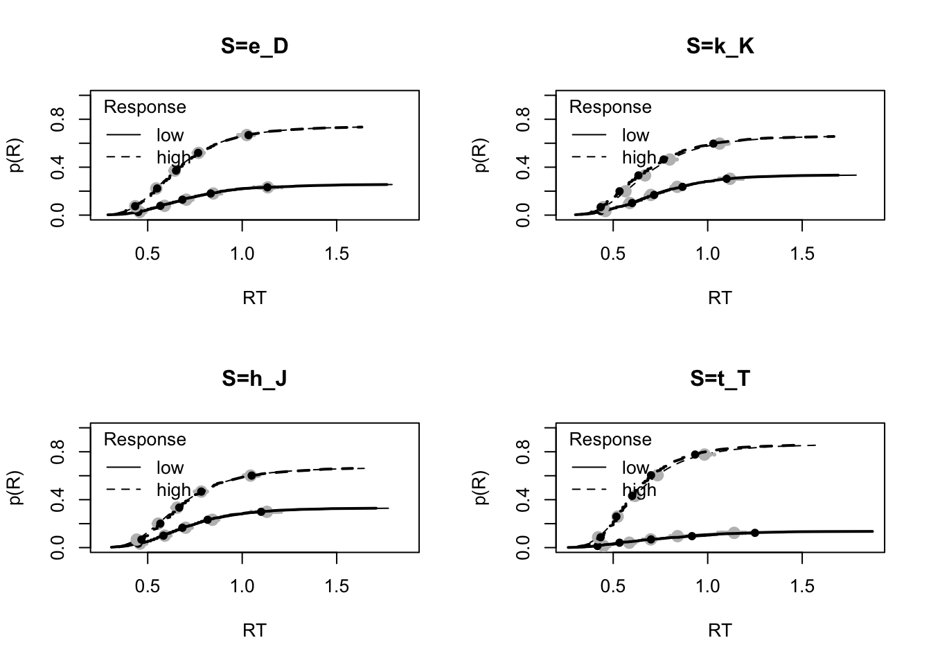

# Priors clearly dominated
ciMiletic1_rdm <- plot_density(miletic1_rdm,layout=c(2,3),selection="mu",subfilter=500)
# Estimates fairly similar to Miletic et al.'s estimates with q0 fixed at zero.

# Plot observed rt and response probability averaged over subjects
plot_adapt(data = data,design=design,do_plot="R",ylim=c(0,1))
plot_adapt(data = data,design=design,do_plot="rt",ylim=c(0.3,1.05))

# Get adaptive estimates and fits to allow plotting of 95% CIs
# Base estimates on posterior means for each participant
pars <- parameters_data_frame(miletic1_rdm,selection="alpha",subfilter=500,stat=mean)
# # This is slow so use pre-computed. Also watch out for RAM use!
# adapted <- plot_adapt(data = attr(miletic1_rdm,"data_list")[[1]],design=design,
#   do_plot=NULL,reps=500,n_cores=11,p_vector=pars)

# Plot adaptive estimates
plot_adapt(adapted=adapted,do_plot="learn",ylim=c(0.1,.85))
plot_adapt(adapted=adapted,do_plot="par",ylim=c(2,5))
# Plot trial fits to rt and response probability averaged over subjects
plot_adapt(adapted=adapted,do_plot="R",ylim=c(0,1))
plot_adapt(adapted=adapted,do_plot="rt",ylim=c(0.45,1.15))
# There is some misfit early in learning 

# save(adapted,miletic1_rdm,ppmiletic1_rdm,
#      file="vignettes/ReinforcementLearning/samples/miletic1_rdm.RData")

#### Parameter recovery study ----

# Simulate data from the posterior means
miletic1_rdm_simdat <- post_predict(miletic1_rdm,use_par="mean",n_post=1,subfilter=500)
# Looks like the real thing.
plot_adapt(data = miletic1_rdm_simdat,design=design,do_plot="R",ylim=c(0,1))
plot_adapt(data = miletic1_rdm_simdat,design=design,do_plot="rt",ylim=c(0.3,1.05))
# If we provide parameters we can see the average learning and rates
plot_adapt(data = miletic1_rdm_simdat,design=design,do_plot="learn",ylim=c(0,1),
           p_vector=attributes(miletic1_rdm_simdat)$pars)
plot_adapt(data = miletic1_rdm_simdat,design=design,do_plot="par",ylim=c(2,5),
           p_vector=attributes(miletic1_rdm_simdat)$pars)



# can we recover these?
miletic1_rdm_sim <- make_samplers(miletic1_rdm_simdat,design,type="standard")
# save(miletic1_rdm_sim,file="miletic1_rdm_sim.RData")
# run in run_miletic1_rdm_sim.R

# Looks fine over last 1500
print(load("vignettes/ReinforcementLearning/samples/miletic1_rdm_sim.RData"))
check_run(miletic1_rdm_sim,subfilter=500)

# Excellent stationary fit
plot_fit(miletic1_rdm_simdat,ppmiletic1_rdm_sim,layout=c(2,2),factors="S")

# Some updating but likely shrinkage influential
tabs <- plot_density(miletic1_rdm_sim,selection="alpha",layout=c(2,3),
                     pars=attributes(attr(miletic1_rdm_sim,"data_list")[[1]])$pars)
# Note mapped=TRUE does not work for adaptive models.

# OK recovery, shrinkage understandable given small sample size per participant
plot_alpha_recovery(tabs,layout=c(2,3))
# Coverage is fairly decent , maybe a bit under
plot_alpha_recovery(tabs,layout=c(2,3),do_rmse=TRUE,do_coverage=TRUE)

# Plot observed rt and response probability averaged over subjects
plot_adapt(data = miletic1_rdm_simdat,design=design,do_plot="R",ylim=c(0,1))
plot_adapt(data = miletic1_rdm_simdat,design=design,do_plot="rt",ylim=c(0.45,1.15))

# Get adaptive estimates and fits, which can be done by providing the samples
# object. We can provided the posterior mean parameters as before by and
# appropriate setting of p_vector (other statistics such as "median" can be 
# used) along with a subfilter if needed. Again stored to avoid slow compute
# adapted_sim <- plot_adapt(samples = miletic1_rdm_sim,do_plot=NULL,reps=500,n_cores=11,
#   p_vector="mean",subfilter=500)

# Plot adaptive estimates
plot_adapt(adapted=adapted_sim,do_plot="learn",ylim=c(0.1,.85))
plot_adapt(adapted=adapted_sim,do_plot="par",ylim=c(2,5))
# Plot trial fits to rt and response probability averaged over subjects
plot_adapt(adapted=adapted_sim,do_plot="R",ylim=c(0,1))
plot_adapt(adapted=adapted_sim,do_plot="rt",ylim=c(0.45,1.15))
# As expected when fitting the true model the misfit has disappeared.

# A better approach to fully represent uncertainty is to sample parameters
# from the posterior (one per rep) as below.
# adapted_sim_sample <- plot_adapt(samples = miletic1_rdm_sim,do_plot=NULL,reps=500,n_cores=11,
#   p_vector="sample",subfilter=500)

# Plot adaptive estimates
plot_adapt(adapted=adapted_sim_sample,do_plot="learn",ylim=c(0.1,.85))
plot_adapt(adapted=adapted_sim_sample,do_plot="par",ylim=c(2,5))
# Plot trial fits to rt and response probability averaged over subjects
plot_adapt(adapted=adapted_sim_sample,do_plot="R",ylim=c(0,1))
plot_adapt(adapted=adapted_sim_sample,do_plot="rt",ylim=c(0.45,1.15))
# In this case there is very little change to the credible intervals.


# save(adapted_sim,adapted_sim_sample,miletic1_rdm_sim,ppmiletic1_rdm_sim,
#      file="vignettes/ReinforcementLearning/samples/miletic1_rdm_sim.RData")