Model Based Sampling with EMC2 - Extended Models of Choice
2022-08-05
Chapter 1 Overview
This project provides a tutorial for learning about cognitive models, namely evidence accumulation models (EAMs), their implementation and their applications. The tutorial was prepared by Andrew Heathcote, Dora Matzke, Russell Boag, Niek Stevenson and Reilly Innes.
The GitHub repository for this project can be found here. The accompanying samples for the code provided here can be found at here.
1.1 Key Terms
Throughout this guide, we’ll use some complex terminology for different aspects of modelling. We know that models exist, and in particular, models of decision making exist, but we want to know how we can connect the models with data. These models have a mathematical structure, which allow a computational account of behaviour, and within this, parameters allow flexibility to account for different types of behaviour under the same formal explanation. How do we then find the best parameters, given our data? And how can we compare competing theories of behaviour? And how well does our model describe the data? For models of choice, this guide will provide a framework for us to answer all of these questions.
Generative Model: A mathematical structure instantiated as a computer program that generates simulated data.
Model Parameters: Variables whose values determine the data generated by the model. The model acts in different ways, depending on the parameters. Can be either fixed a priori (constants) or determined based on empirical data (estimated parameters - these allow flexibility). These might be varied to test competing theories.
Model Estimation: A complex process of choosing a set of parameter values that provides the best match between some observed data and the data generated by the model. This is complicated because the models are flexible, so could account for the data in a number of ways. When estimating parameters, we want to be able to use the estimates to test our theory, i.e., condition 1 should be higher in parameter x than for condition 2. As the parameters have psychological meaning, we may need to constrain these parameter estimates.
Fit Metric / Objective Function: A measure of the quality of the data-model match (“goodness-of-fit” or “deviance”). Here we can also think about phenomena such as “over-fitting” our models or allowing for greater flexibility.
Model Selection: A method of selecting from a set of estimated models the one that is “best” in the sense of matching both that data from which it was estimated and potential future data it aims to explain.
Parameter-based inference: Inferences about (latent) psychological processes made directly based on parameters that describe them rather than indirectly based on directly observed (manifest) behaviour. Related to model estimation, we can test whether parameter x is greater in condition 1 or 2.
Sampled/Sampling: When we estimate the model, we use an MCMC process which proposes potential ‘good’ parameter values (for the model given the data). On each iteration of this process we take a “sample”, and hence, we refer to “sampling” as the process of obtaining samples (fitting the model) and “sampled” as an object that has been sampled.
Transformations: Models often use parameters that are on a certain scale. For example, a probability estimate may be between 0 and 1 and some parameters may need to strictly positive (i.e., response time cannot be negative). When estimating the model, samples are given on the real line (-Inf to Inf), meaning that we may need to transform some of these parameters so that the model can actually use them (and avoid returning NaN’s and infinite values).
Natural scale: Following transformations, we refer to the natural scale as the scale used by the model. Hence if the probability parameter was p = 0.5 on the natural scale (and a probit transformation was used), we could know that the sampled value was qnorm(0.5) and the estimated probability parameter as used by the model was 50%.
Sampled scale: The sampled scale is the opposite of the natural scale. These are values that are the actual values sampled before any transformations have been done.
Mapping: Mapping is referred to throughout as the process by which we take parameters (such as intercept and effect terms) and map these to conditions. This means that in each cell of the design, we get a mapped parameter, such that it is assigned the correct values as we intended. For example, condition 1 should get the corresponding parameters for conditions 1 (including any calculations such as mean + effect terms).
1.2 “All models are wrong but some are useful” – Box, (1979)
Importantly, many of the models discussed in this guide should be considered as just that - models. Models are not the system that they are modelling, but rather an abstraction of that system. Like a model train does not represent a real train, models ignore some parts of the environment in order to understand the main system of interest. However, these models allow us to extract information in order to explain unobservable phenomena.
1.3 Computational Cognitive Models
Computational cognitive models are used to represent latent cognitive processes underpinning observed behaviour. We can use models as tools to gain further insight into data from behavioural experiments. This means that rather than just assessing descriptive statistics, such as means of choices or response times across conditions, we can model the data, parameterising our models in such a way that these mathematical models resemble a cognitive process.
For a simple example involving Signal Detection theory, see here
1.4 Uncertainty and Noise in Models of choice
When analysing observed behaviour, we tend to observe noise in the behaviour (and measurement). For example, when responding to a stimuli repeatedly, some of our responses may be fast, whilst other responses may be slower. Over many responses, we’ll build up a distribution of response times (RT). When formalising our model, and estimating the parameters of the model, we want to be able to capture this noisy distribution as best we can. For this, we can use distribution functions.
1.4.1 Distribution Functions
Here we describe some concepts that are key to our modelling approach.
Normal distribution: the sum of many small uncertainties (i.e., like the example of RTs above).
Typically associated with the frequentist perspective and the means of measurements due to the central limit theorem: the distribution of sample means approximates a normal distribution as the sample size gets larger, regardless of the population’s distribution (i.e., of epistemic uncertainty).
Density: The instantaneous probability of getting a number. In the example figure, 0 is highly likely, whereas 4 is very unlikely. Density functions in R are written as d-dist, for example for a normal distribution, this is dnorm. The function pnorm on the right, is the integral of the function dnorm on the left. Note that pnorm is often called a “probit” transformation and used to project a bounded variable to the real line. Logarithms are used for a similar purpose when only one end is bounded.
Random Generation: On the other hand of density functions are the random generation functions (written as r-dist in R). These functions similarly take in parameter values, but rather than calculating the density, instead generate values by drawing from the theoretical distribution.
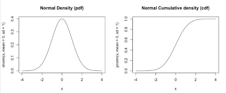
Figure 1.1: Example Distributions
1.5 Likelihood and Probability Density
Before we dive into model-based sampling any further, it’s important to understand the engine to model-based sampling; likelihoods.
The likelihood is a probability measure, where higher likelihoods indicate higher probability. When estimating a model given some data, we want to find the parameters of the model that best describe the data. For example, if our data was normally distributed, we might want to find what the mean and sd were, so we could use the dnorm function and test lots of different mean’s and sd’s until we found the values with the highest likelihood. This process is akin to what we do in model-based sampling, where we search for likely parameters, given our models.
However, not all models will have such straightforward (and analytically solvable) density functions. In EMC2, we generally use models where the likelihood can be directly computed. Further, in EMC2 we often want to compute the differences in parameters across conditions - i.e., not just mean and sd overall, but a difference in parameters across conditions. EMC2 gives us a method of achieving this.
1.6 Introduction to Model-Based Sampling
Model-based sampling is the process of model estimation given some data. For this exercise, we propose a model (and parameterisation) and then estimate the values of the parameters given the data to find the “best fitting parameters” - which means the most likely parameters. EMC2 is designed to facilitate model-based sampling. Here, we use state-of-the-art sampling methods that are robust, efficient and reliable. These methods include both hierarchical and single-subject sampling schemes. The sampling scheme used for hierarchical modelling also allows for different group level parameterisations, however, the standard method shows an advance on other sampling methods (such as DE-MCMC and STAN) by estimating a group level multivariate normal model, which allows us to estimate the means of parameters and the correlations between parameters. This method is known as particle metropolis within Gibbs sampling (PMwG).
To estimate the models and reach the posterior, we use an MCMC sampling method. For this sampling method we draw a number of proposals (particles) at each step (iteration) and select the best particle (relative to the previous run) for each participant. The rate of new particles taken for each subject is termed “acceptance”. We tend to aim for around 60% acceptance. To start, we sample some start points from the prior. We then do a period of “burn-in”.
The burn-in period is used to get the sampler to a “good” area of the sampling distribution which is close to the posterior. When the samples have reached the posterior and are stationary, we term this “convergence”. For PMwG, we often see that the sampler reaches this point relatively quickly (~100 iterations). We know the sampler has reached this area when the samples are stable. To see stationarity, we view parameter chains. These parameter chains are the sampled values for each iteration for each parameter. We can see stationarity when the chains appear to be flat, with no slope. These chains should also include some variance, so may resemble “hairy caterpillars”.
Following burn-in, the sampler has two other stages – adaptation and sampling. The adaptation stage creates a more efficient sampling distribution for each subject, whilst the sampling stage draws samples from this efficient distribution and these are the posterior samples we make inference on.
Rather than using point estimates, we use many samples from the posterior so that we create a posterior distribution. We can then asses the mean or median of this distribution to make inference about parameter values and differences, as well as the variance, so that we can account for certainty in the model. We only use samples from the posterior distribution for this, as these are the samples with the highest likelihood, and therefore, the most representative. That is, we fit a model and obtain estimates of its parameters that best describe the data by sampling from the model.
1.6.1 Single Subjects and Group Levels
In EMC2, we show two types of sampling methods, single subjects or hierarchical. In single subjects sampling, we aim to find the posterior likelihood of each subject’s parameters, conditional on the data. For hierarchical, we aim to find the posterior likelihood of the population parameters, conditional on the estimates of each subject’s parameters.
For single subjects sampling, each subjects’ parameters are sampled independently for each subject, accounting for the prior. There are some advantages for single subject sampling in that we can efficiently sample parameters for each individual, which is especially useful with low sample sizes. In EMC2 for single subject sampling, on each iteration for each individual, the proposal particles are sampled from both a distribution centered around the individuals’ previous accepted particle and samples from the prior. This means that there is some “protection” for individuals if their estimates are “stuck” in a bad area by using the prior. This can however be slow to converge.
For hierarchical sampling, there are other benefits and limitations. In hierarchical sampling, we assume that each individual is part of a population, where the population influences individuals’ parameter estimates and individuals influence the population parameter estimates. In hierarchical sampling, we often make inference on the group level, as this is informed by each participant. This means that participants who have parameter estimates far away from the group have less impact over the results. Similarly, the group level imposes constraints on the individuals, such that individuals with more extreme parameter estimates are pulled closer to the group – this is known as “shrinkage”. In EMC2, on each iteration for each individual, the proposal particles are sampled from both the group level distribution and a distribution centered around the individuals’ previous accepted particle. This means that there is some “protection” for individuals if their estimates are “stuck” in a bad area by bringing them closer to the group distribution. This also means that convergence is faster.
1.6.2 Priors
In a hierarchical model we assume that each subject’s parameters are sampled from population distributions. For an introduction to the benefits of such models see Shiffrin, R., Lee, M., Kim, W., & Wagenmakers, E.-J. (2008). A Survey of Model Evaluation Approaches With a Tutorial on Hierarchical Bayesian Methods. Cognitive Science: a Multidisciplinary Journal, 32(8), 1248–1284.
For all the model sampling we show here, we use Bayesian estimation methods. This means that the likelihood of each parameter proposal takes into account the prior. In many Bayesian applications we may have to decide what prior we use. This prior relates to the distribution from which parameter values are sampled. That is, our parameters are treated as random variables having their own associated probability distributions. For example, t0 could not have negative values (as it relates to non-decision time), so often a truncated normal distribution is used.
For PMwG, we use a multivariate normal distributed prior across parameters. This means that some values need to be transformed (like t0). The prior constrains the values that are proposed. This means that the prior should include any reasonable values. If the “true” values are outside of the prior, the values estimated will be in the tails of the prior. Hence, any estimated values that are against the prior means that we should broaden or shift our prior. An example of this can be seen below.
1.6.2.1 Single subject priors
The prior for single subjects sampling is somewhat simpler in that we need not account for the group level distribution. Here, parameters are sampled from a normal distribution for each parameter.
1.6.2.2 Transformations and Implied Priors
EMC2 estimates values on the real line, so for many parameters, transformations are required. However, in transforming the values of these parameters, we now have a different implied prior. For many of our transformations, an exponential transform is used (i.e., exp), such that parameter values are strictly positive. When considering the output of the sampler, we should consider these values on both the real line and natural scale. On the natural scale, this means we also need to attain our implied prior.
1.6.2.3 Alternate Group Level Priors
EMC2 also offers users the flexibility of specifying alternate group level models. These alternate group level models make different assumptions about the distribution of group level variances, where the variance is changed from a variance-covariance matrix. The different types of models include Factor Analysis, Blocked Covariance, Independent and Factor Regression. Each of these uses a different group level prior, specifically for the covariance matrix. The user need not make any changes to these alternate model priors, which are included in the code. For more on the alternate group level models, see Advanced.
1.6.3 Posterior
The posterior is our target distribution. The posterior mode contains the values which are most likely (given data and priors). To reach the posterior, we need to take many samples from the proposal distribution to ensure we have explored the entire space and found the region which contains the most likely parameters. This relies on an updating process which is explained above. When the sampler has converged on the posterior, we can draw samples from this region which we use to make inference. We will show diagnostic measures to ensure convergence later on, but think of this simply as a region where the likelihood is highest and parameter estimates are stable (with some noise due to sampling variability).
Using these samples, we can make inference on the location and variability. For the location, we may wish to draw inference on between condition parameter estimates, so here we can evaluate the differences between parameters. Further, we can do this with a margin of error because we have many posterior samples that form a distribution. If the distribution is wide, we will have less certainty and vice-versa.
1.6.4 Likelihood
Calculating the likelihood is key to the sampling process. In hierarchical sampling we have two types of posterior likelihood to consider: (a) The posterior likelihood of each subject’s parameters, conditional on the data (b) The posterior likelihood of the population parameters, conditional on the estimates of each subject’s parameters.
For (a), this is the same as in the single subject case (but with one instance for each subject), except that the prior is calculated relative to the current estimates of the population parameters (i.e., it changes over MC iterations)
For (b) we need to specify a prior for the population parameters (which does not change over iterations). The relevant likelihood is of the current parameters for each subject (which do change over iterations) under the population model.
This means that for each proposal, the likelihood is estimated conditional on the data for each subject, as well as conditional on the group level distribution, where the group level distribution is conditional on the prior (hence the hierarchy).
1.6.5 PMwG Specific
EMC2 uses the PMwG sampling algorithm (Gunawan et al. 2020) for hierarchical sampling and a modification of this for single subject sampling. In PMwG, on each iteration, a number of particles are generated that represent proposals for each participants’ parameters (alpha). These particles are n parameters long, and are compared to each other, as well as the previous most likely particle. If a proposed particle is more likely than the previous iteration, it is kept to the next iteration, and the process continues until the posterior is reached.
A key difference in the hierarchical and single subject sampling schemes is where these proposals are generated from. For hierarchical sampling, a proportion of particles is generated using values from the group level and from the individuals’ previous best particle. In single subject, rather than proposals from the group, a small proportion are sampled from the prior.
There are many more nuances and deeper details involved in the sampling algorithm and the group level models used, which can be seen in Gunawan et al. (2020) and in the PMwG samplers documentation. For EMC2, this algorithm and sampling functions are hidden to the user, so all that matters is how to use the code, how to diagnose problems and how to interpret the output. For the output, there are three key areas of interest, subject level parameters (also known as random effects or \(\alpha\)), group level mean parameters (\(\theta_\mu\)) and group level variance covariance parameters (\(\theta_\Sigma\)).
1.6.5.1 Priors
Gunawan et al. (2020) proposed priors for PMwG, which we follow in EMC2. Most of these prior settings are hard coded as they are broad and accommodate the vast majority of estimation exercises. The location of these priors can be set with reasonable prior knowledge, however, the general setting of 0 is typically fine for EAMs. Further, we would warn against changing the variance parameters as this is both more difficult and has further consequences for the implied prior.
In PMwG, the prior for the group level is a multivariate normal distribution, with mean \(\mu\) and covariance \(\Sigma\). The mean of the group level is assumed to be another multivariate normal distribution, with mean (location) default set to 0 (but can be changed) and the variance an identity matrix. The prior on the covariance is specified by Huang and Wand (2013), using a mix of inverse Wishart distributions with mixture weights given by an inverse Gaussian distribution. Using Huang and Wand (2013) leads to marginally non-informative priors on the correlation coefficients and half-t distributed priors on the standard deviations (Wall et al. 2021).
These are all hard coded into the PMwG algorithm (for the standard group level model) and generally require no user interaction or changes. As noted above, there are alternate group level models available in EMC2, however, the priors for these models are also hard coded and require no user interaction. Consequently, for EMC2, the only choices required from the user regarding priors are; (a) what group level model to use – e.g., standard, factors, independent (diagonal), etc; (b) whether there is evidence to suggest the location prior of \(\mu\) (i.e., theta_mu_mean) needs to be specified.
1.6.5.2 Subject estimates
For the subject level estimates \(\alpha\), the sampler returns a matrix of size subjects x parameters x iterations. Looking at the posterior, we can evaluate each subjects’ best fitting parameters conditional on the data and influenced by the group level parameters. We can use these estimates to perform inference at the subject level, or, more importantly, generate posterior predictive data.
Posterior predictive data is often used to evaluate model fit. Here, we take random samples of \(\alpha\) for each subject from the posterior. Using these samples, we generate data as outlined above. We can then compare the generated data to the observed data to see how well the model fits the data.
1.6.5.3 Group Mean
We often conduct the majority of our inference on the group mean (\(\theta_\mu\)). The sampler returns a matrix of size parameters x iterations. The group mean is often called the “hyper” level distribution. A lot of diagnostic checks are conducted on samples from this level. This is because we are most interested in effects at the group level. These are the parameters used for most tests, especially across conditions, where we may investigate the difference in a given parameter due to a manipulation.
1.6.5.4 Covariances & Correlations
Finally, PMwG also estimates a variance covariance matrix (\(\theta_\Sigma\)). This matrix is size parameters x parameters x iterations, where a matrix is given for each iteration. Here, we can see the within parameter variance over the group for each iteration (on the diagonal) and the covariance between parameters for off-diagonal cells. Further, we can easily transform this into a correlation matrix, where we can look at the distribution of correlations across iterations to make inference about relationships between parameters. This is especially useful for models with high colinearity and joint-models.