Chapter 8 Joint Models
Joint models are models which combine multiple sources of data, or multiple models of different sources of data. For instance, let’s say we have an experiment where participants complete two behavioural tasks. Task 1 is a memory task and Task 2 is a working memory task. To analyse this data, we could assess correlations to understand the links between tasks. If you are good at long term recognition memory, maybe you are also good at working memory? Let’s assume we are using a model-based design, because we want a deeper insight into the latent variables underpinning behaviour in this task, so we will use decision making models for each task.
If we do sampling for both models, then look at the correlations, these are likely to be attenuated (for more on this see Matzke et al. 2017). This means that any true correlations that exist will be underestimated and may wash out in the analysis. Further, because the same people are doing the tasks, and we can assume that there are similar processes being employed for each task (i.e., decision making tasks), then we could model the behaviour in a joint fashion. For this, we would not want a single model to describe both data sets - we know these are fundamentally different. So we need to come up with a “joint model” that allows us flexibility to assess relationships that may exist.
8.1 Types of Joint Models
There are many types of joint models, which are introduced concisely in Turner 2015?. These can be broken into three main categories; directed joint models, covariance joint models and integrative joint models.
8.1.1 Directed joint models
Directed joint models use data from one source to directly inform the other model. For example, one might take neural activity (either direct measurements or a model of this) and use it to inform parameters of another model. If we can use something like a direct measurement of neural activity to inform a parameter like drift rate in a decision making model, this means we have less parameters to estimate, and a direct link between the two sources of data. Here, we can directly test hypotheses we may have about one source of data informing the other. However, this is problematic due to the strong assumptions that need to be made.
8.1.2 Integrative joint models
Integrative joint models assume that the data is the result of a single integrative model. These models are highly appealing as they provide a “single model to rule them all”. This means that one process leads to all the data. However, for this type of model, it is very rare that one model could describe all the data, at least for tractable models that we fit in EMC.
8.1.3 Covariance joint models
Covariance joint models are models where the group level model provides a link between subject level models/sources of data. This means that we can have a model for each component of the data (i.e., Task 1 and Task 2 components) and estimate a group level model which accounts for both underlying models. This is implemented through estimating a covariance matrix. In estimating a covariance matrix, we can directly estimate the correlations between model parameters across components, such that if parameters are in some way dependent, we will observe correlations between these parameters.
8.1.4 Seminal work from Wall facilitated by Gunawan/PMwG
Wall et al., (2021) used the covariance matrix in their study to show correlations in parameters across behavioural tasks. This seminal work of behaviour-behaviour modelling highlighted the strengths of the covariance matrix, where the group level model showed positive correlations between threshold parameters across tasks. This result indicated that participants set similar thresholds across the different tasks. This example provides a clear, data-driven result for assessing the “joint” nature of behaviour, where we can assume that behaviour is related across tasks.
Additionally, the work by Wall et al., (2021) was one of the first practical psychological applications of the PMwG sampler (which underpins EMC sampling). The strength in the standard PMwG approach comes from both the group level model estimation, where the group level model assumes a multivariate normal distribution of parameters, and from the particle sampling, where proposed particles include the full vector of parameters to be estimated, meaning that colinearity is accounted for (i.e., parameter estimation is not done independently). Here, the group level multivariate normal model of parameters includes estimation of the mean (which can be used for inference on parameter differences), and importantly, a covariance matrix. Here we can use the covariance matrix to estimate correlations between parameters.
8.2 Covariance Matrix
In a joint model using the standard PMwG approach, if we simply combine the vectors of parameters to be estimated for each model, we now have a larger vector of parameters to estimate for each particle, a larger vector of mean parameters and a larger covariance matrix. Within this covariance matrix, the off diagonal rectangles provide estimates of the covariances (and correlations) between parameters of the different models. This means that in Task 1 and Task 2, if we had parameters;
$= v_{Task1}, b_{Task1}, t0_{Task1}, v_{Task2}, b_{Task2}, t0_{Task2} $
Then we could look at the relationships between \(v_{Task1}\) and \(v_{Task2}\) etc. A graphical example of this structure can be seen below;
FIGURE
8.2.1 Why so useful?
This group level model estimated by PMwG is highly useful to (covariance) joint modelling applications, as it allows us to estimate a covariance matrix within the group level model, on which inference can be made. Further, there are no specific assumptions that are required and we can rely on models that are unique to each data set. This means that we could use any subject level model, as long as each subject had data for each component. For example, we could estimate a model of the decision making behaviour using the LBA and a model of neural activity using a regression model. Then after sampling the model, we could assess the correlations between estimated drift rates and beta’s (for example).
Importantly, estimating a covariance matrix limits the potential attenuation of correlations. As shown in Matzke et al. (2017), when correlation statistics are taken for point esitmates, correlations tend to be attenuated. For example, if we estimate a model for two tasks and then correlate the median posterior parameter estimates, these can be attenuated as it does not account for the full distribution, or for the measurement noise. You can think of it this way, if we don’t take into account for the noise in our measurement, all that noise will end up diluting our correlations. However, if we estimate the correlations (i.e., a covariance matrix), then this implicitly accounts for any measurement noise and provides an estimate of confidence around the correlation, i.e., a credible interval on the correlation estimate. This means when estimating the distribution of correlations, we not only observe the median correlation (which no longer suffers from attenuation), but we can also see the spread of this estimate, where a peaked distribution would indicate a higher confidence, whereas a distribution with greater spread would show us greater confidence in that estimate.
Evidently, the covariance matrix estimated as part of the group level model is highly useful for joint modelling applications. This also means we have a data driven model, as opposed to relying on specific hypotheses about links between the data. In later lessons, we’ll also give some insight into new methods for parameterising the group level model, such as using factor analysis rather than a covariance matrix.
8.2.2 Why not used before?
Previous attempts had been made at estimating a covariance matrix, however, often these were limited by the sampling approach. For example, in DE-MCMC, we could estimate a multivariate group level model, however, there were issues with estimation. Further, the PMwG algorithm enforces dependence of parameters, as we propose vectors of parameters (particles) on each iteration, rather than independently estimating parameters. Evidently, this highlights that PMwG is a state of the art sampling method, which is why we use this as the engine for EMC.
8.3 Exercises
Here we show two joint modelling exercises. These two examples are examples of standard joint modelling examples one may wish to run. The first is a behaviour-behaviour joint model and the second is a joint model of behavioural and neural data. For the behaviour-behaviour joint model, we have behavioral data for a within-subjects design, where each participant completed two tasks (or in this case, the same task across two environments).
There are many potential uses for this kind of joint modelling - across multiple tasks, environments, instruction manipulations, days of the week etc. As long as each subject has data in each cell, we could fit a joint model across the space and then assess the correlations between parameters. This would allow us to answer questions like, “Is drift rate correlated over days of the week?” or “Does threshold change between tasks?”. Using this approach, we could assess correlations between parameters to make inference on whether participants who have high drift rate in one task, have high drift rates in another task.
For the neural-behavioural joint model, we apply this approach to data collected within a fMRI scanner, where each participant has both behavioural data and functional imaging data. Here, we can model the contrasts, and model the behavioural data, and then use the covariance matrix to assess relationships between these sources of data. Often researchers only show descriptive statistics (i.e., threshold went up in condition x and so did activation at location y) or post-hoc correlations. However, this is problematic as it uses point estimates, which fails to account for the measurement noise we might experience in the study. By modelling this data, we can provide an estimate for distributions of data, which inherently suck up some of that measurement noise. In estimating correlations on these parameters, we can then get an estimate of the correlation between parameters, to make stronger inference on correlations that do not suffer from attenuation.
8.3.1 Behavioural x Behavioural Data
In this behaviour-behaviour design, we again use data from the Forstmann, et al. (2008) study, however, this time, we also include the “out-of-scanner” data. For this data, participants completed the same experiment both in and out of an MRI machine. Previously, studies have shown t0 and threshold increases, as well as a slight decrease in drift rate. This makes sense given the environment might be more distracting to the participant. However, we want to look at the links between these tasks. For example, is threshold even related? It could be that thresholds are not linked across the contexts, and by chance they appear lower when looking at point estimates. Using the correlation approach, we can look at the correlations between parameters across the environments, to make stronger inference on within-subject performance consistency.
To do this, we’re going to fit the same model to both contexts. Then, we’re going to join the models together. In EMC, we use a trick where we first get to the posterior of each individual model, and then sample them together for efficiency (in case one model dominates the other/s). Let’s first load in the data and set up the designs.
rm(list = ls())
source("emc/emc.R")
source("models/RACE/LBA/lbaB.R")
load("Data/PNAS_InAndOut.RData")
data$R <- as.factor(data$resp)
data$subjects <- data$subject
data$E <- as.factor(data$cond)
data <- data[,c("subjects", "R", "E", "scan", "rt")]
For our designs, we need a design for each component, so let’s set these up to have the same parameterisations;
# Average rate = intercept, and rate d = difference (match-mismatch) contrast
ADmat <- matrix(c(-1/2,1/2),ncol=1,dimnames=list(NULL,"d"))

Emat <- matrix(c(0,-1,0,0,0,-1),nrow=3)
dimnames(Emat) <- list(NULL,c("a-n","a-s"))


dat1 <- data[data$scan == 0,]
design_ses1 <- make_design(
  Ffactors=list(subjects=unique(dat1$subjects), E=unique(dat1$E)),
  Rlevels=levels(dat1$R),
  Clist=list(R=ADmat, E=Emat),
  Flist=list(v~E*R,sv~R,B~E,A~1,t0~1),
  constants=c(sv=log(1)),
  model=lbaB)
## v v_Ea-n v_Ea-s v_Rd v_Ea-n:Rd v_Ea-s:Rd sv_Rd B
## 0 0 0 0 0 0 0 0
## B_Ea-n B_Ea-s A t0
## 0 0 0 0
## attr(,"map")
## attr(,"map")$v
## v v_Ea-n v_Ea-s v_Rd v_Ea-n:Rd v_Ea-s:Rd
## 41 1 0 -1 -0.5 0.0 0.5
## 101 1 0 -1 0.5 0.0 -0.5
## 1 1 0 0 -0.5 0.0 0.0
## 61 1 0 0 0.5 0.0 0.0
## 21 1 -1 0 -0.5 0.5 0.0
## 81 1 -1 0 0.5 -0.5 0.0
##
## attr(,"map")$sv
## sv sv_Rd
## 41 1 -0.5
## 101 1 0.5
##
## attr(,"map")$B
## B B_Ea-n B_Ea-s
## 41 1 0 -1
## 1 1 0 0
## 21 1 -1 0
##
## attr(,"map")$A
## A
## 41 1
##
## attr(,"map")$t0
## t0
## 41 1dat2 <- data[data$scan == 1,]
design_ses2 <- make_design(
Ffactors=list(subjects=unique(dat2$subjects), E=unique(dat2$E)),
Rlevels=levels(dat2$R),
Clist=list(R=ADmat, E=Emat),
Flist=list(v~E*R,sv~R,B~E,A~1,t0~1),
constants=c(sv=log(1)),
model=lbaB)## v v_Ea-n v_Ea-s v_Rd v_Ea-n:Rd v_Ea-s:Rd sv_Rd B
## 0 0 0 0 0 0 0 0
## B_Ea-n B_Ea-s A t0
## 0 0 0 0
## attr(,"map")
## attr(,"map")$v
## v v_Ea-n v_Ea-s v_Rd v_Ea-n:Rd v_Ea-s:Rd
## 21 1 -1 0 -0.5 0.5 0.0
## 81 1 -1 0 0.5 -0.5 0.0
## 1 1 0 0 -0.5 0.0 0.0
## 61 1 0 0 0.5 0.0 0.0
## 41 1 0 -1 -0.5 0.0 0.5
## 101 1 0 -1 0.5 0.0 -0.5
##
## attr(,"map")$sv
## sv sv_Rd
## 21 1 -0.5
## 81 1 0.5
##
## attr(,"map")$B
## B B_Ea-n B_Ea-s
## 21 1 -1 0
## 1 1 0 0
## 41 1 0 -1
##
## attr(,"map")$A
## A
## 21 1
##
## attr(,"map")$t0
## t0
## 21 18.3.1.1 Combine Designs
Now, you might be wondering how we take these two separate designs and make them into one object to estimate. We’ve built in a “trick” to make this as simple as possible. Simply make a list of the designs you wish to estimate using the functions below. This means you only need a model of each “component” to fit the joint model. Here, we define a component as one piece of the joint model – i.e., a model of data from one part, which could be task 1, or could be behavioural data (compared to neural data).
These functions will combine the designs to make a single model to be estimated. This means on each iteration, the proposed parameters will be for all components. If we had two component models with 7 parameters each, we would estimate 14 parameters per iteration. It is important to note the ordering of the joint model too. EMC will name each parameter as “1|parameter_x” for component 1, “2|parameter_x” for component 2 and so on.
samplers <- make_samplers(list(dat1, dat2), list(design_ses1, design_ses2),type="standard",rt_resolution=.02)8.3.1.2 Sample
Sampling is the same as we’ve shown before. Simply run the code to sample the joint model.
samples <- run_emc(samplers, nsample = 2500, cores_for_chains = 1, cores_per_chain = 20, verbose = T, verbose_run_stage = T)Let’s load in the pre-sampled data instead;
load("~/Desktop/emc_advanced/vignettes/JointModels/samples/joint_PNAS.RData")We also check whether our chains converged;
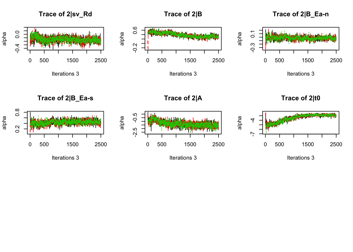
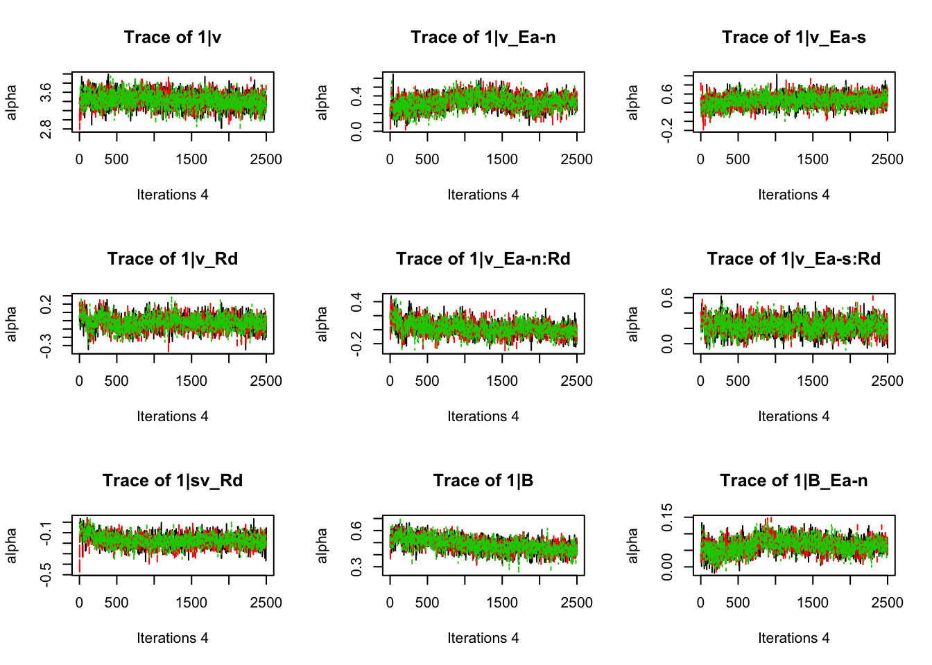
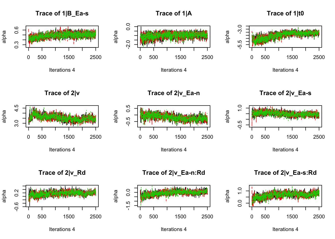
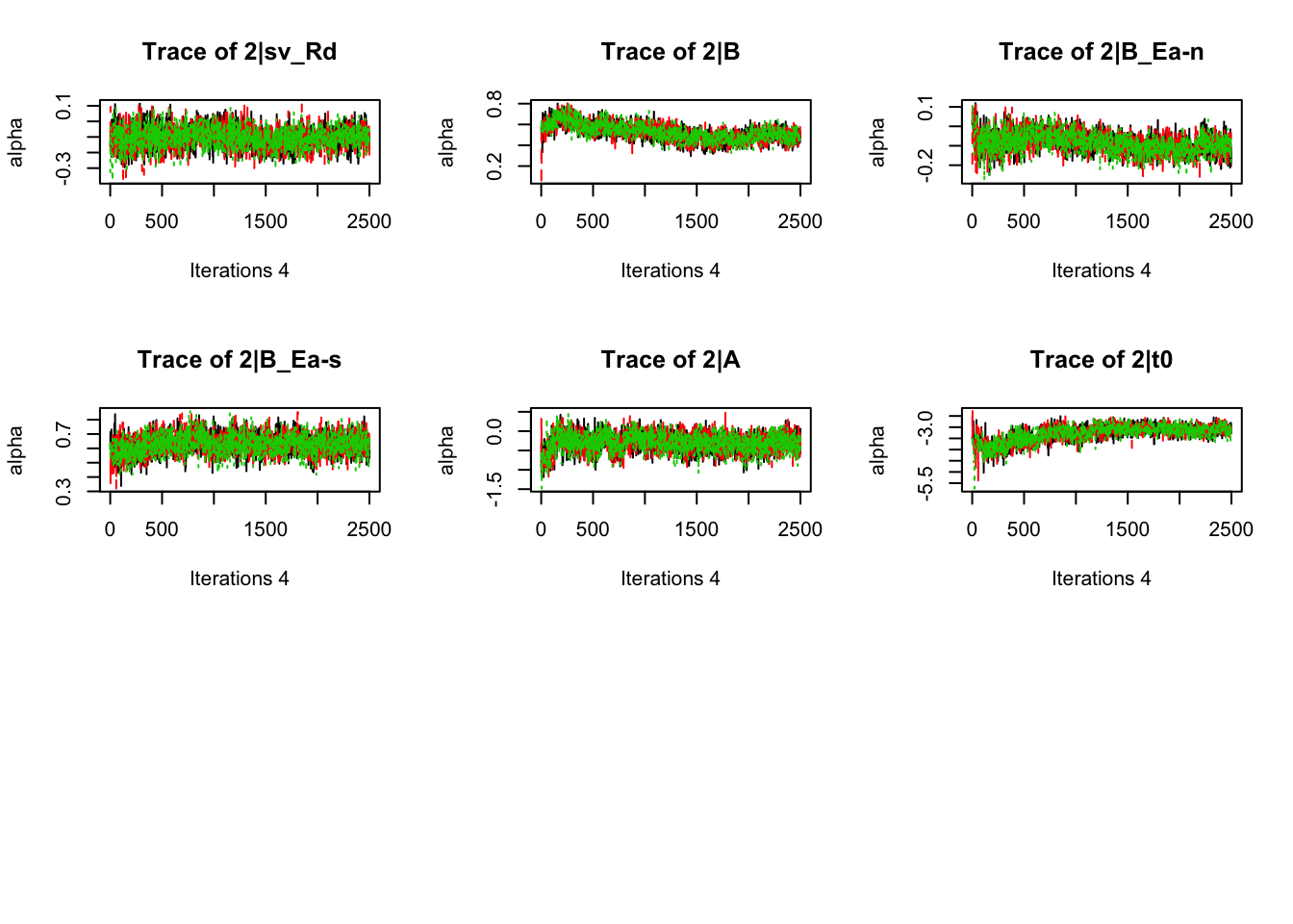
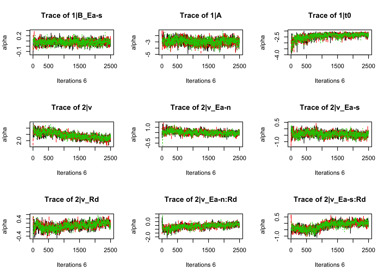
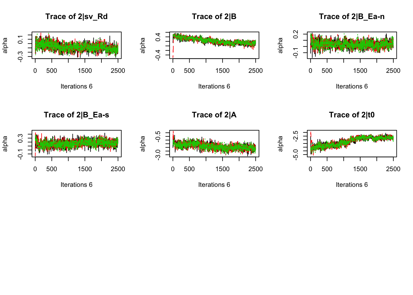
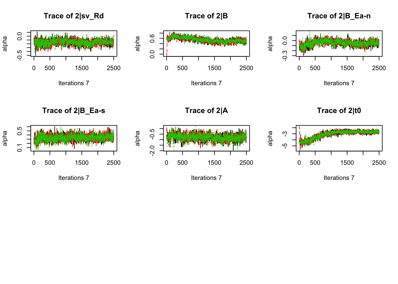
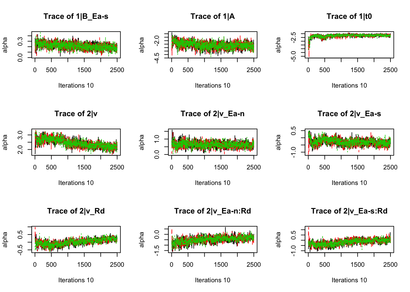
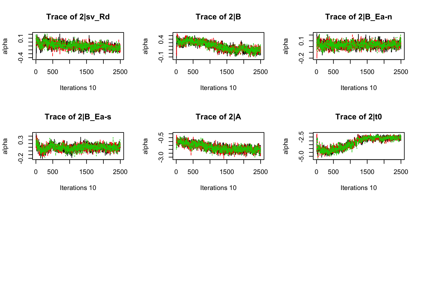
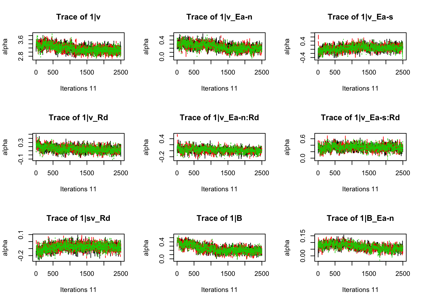
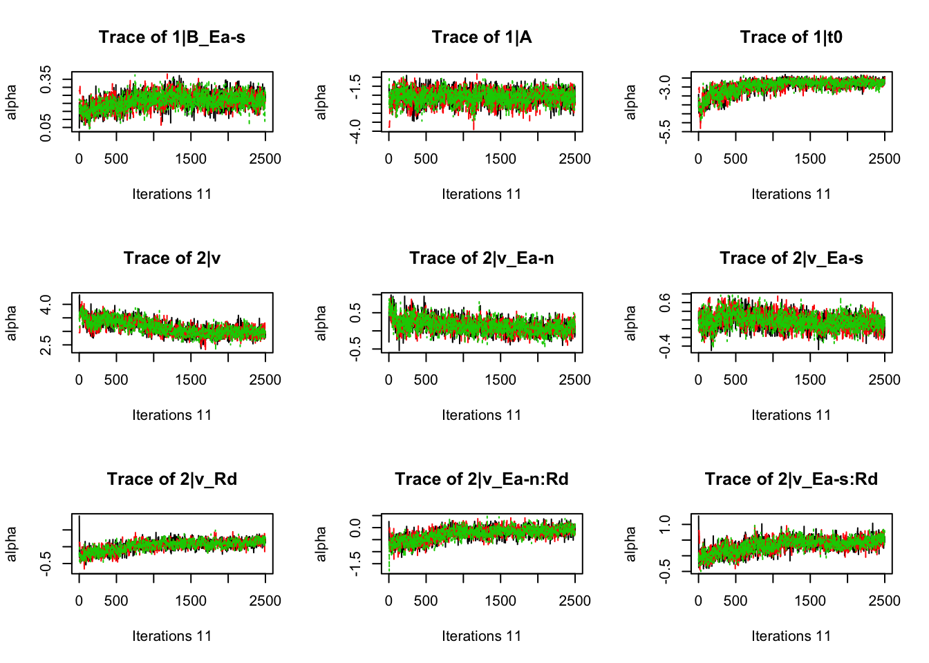
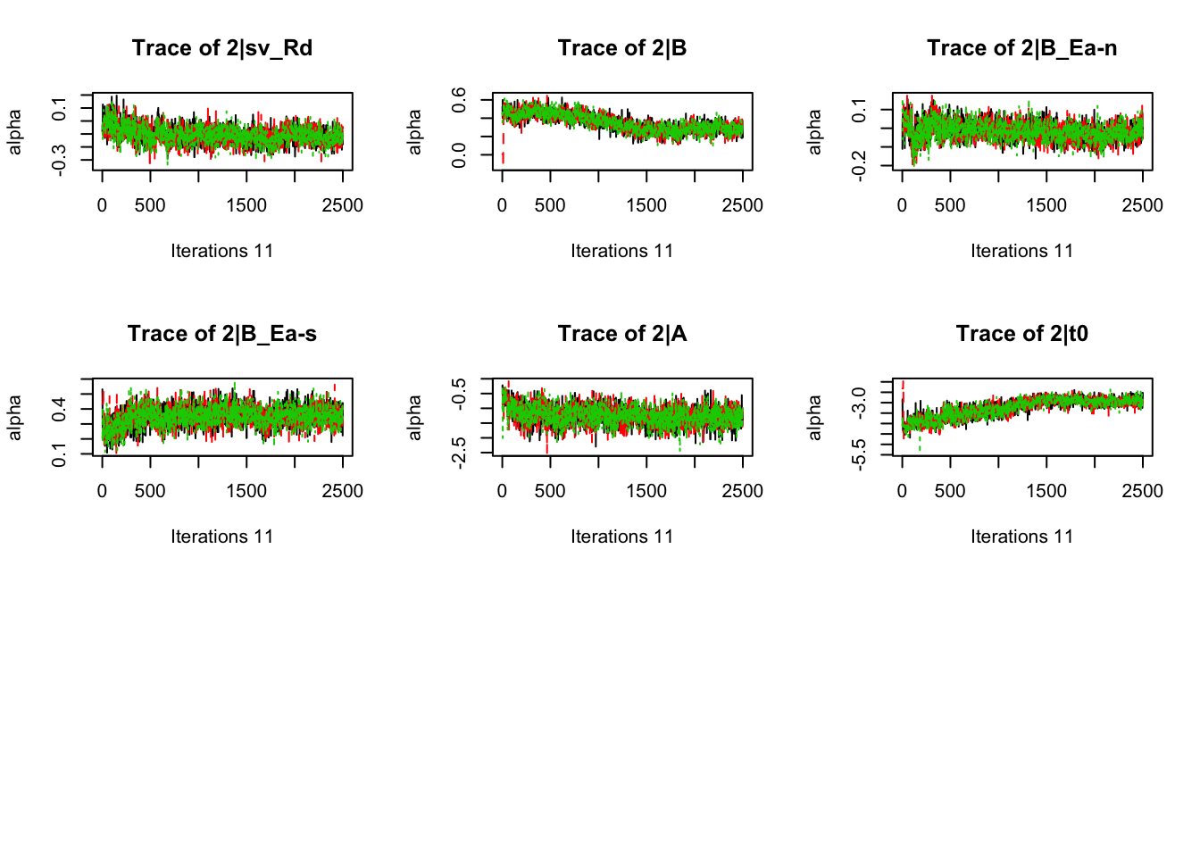
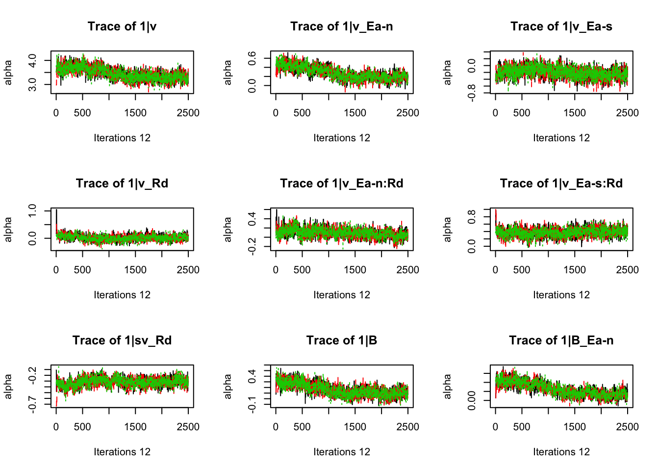
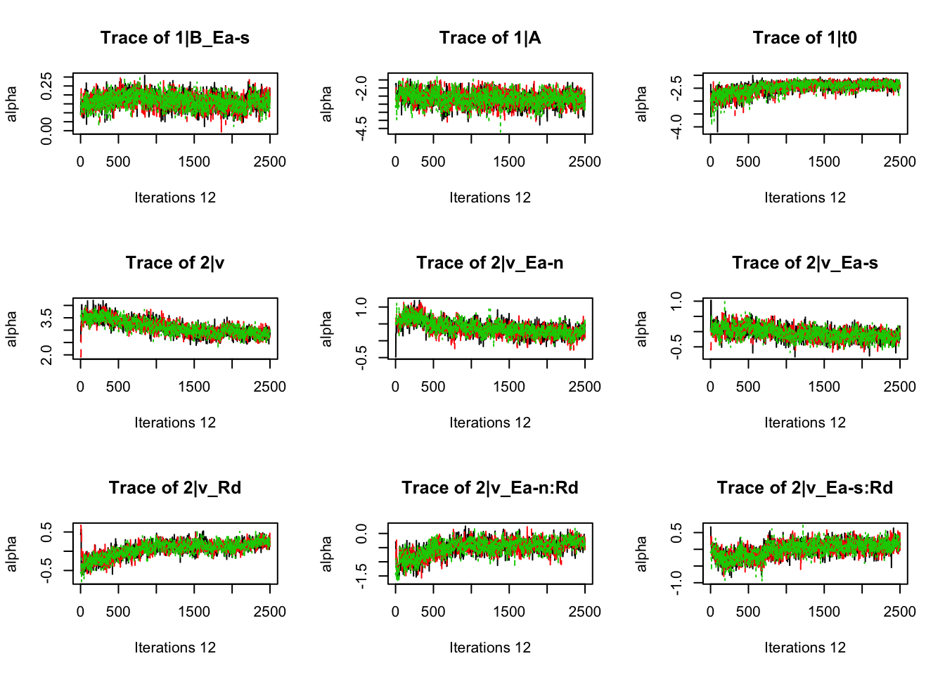
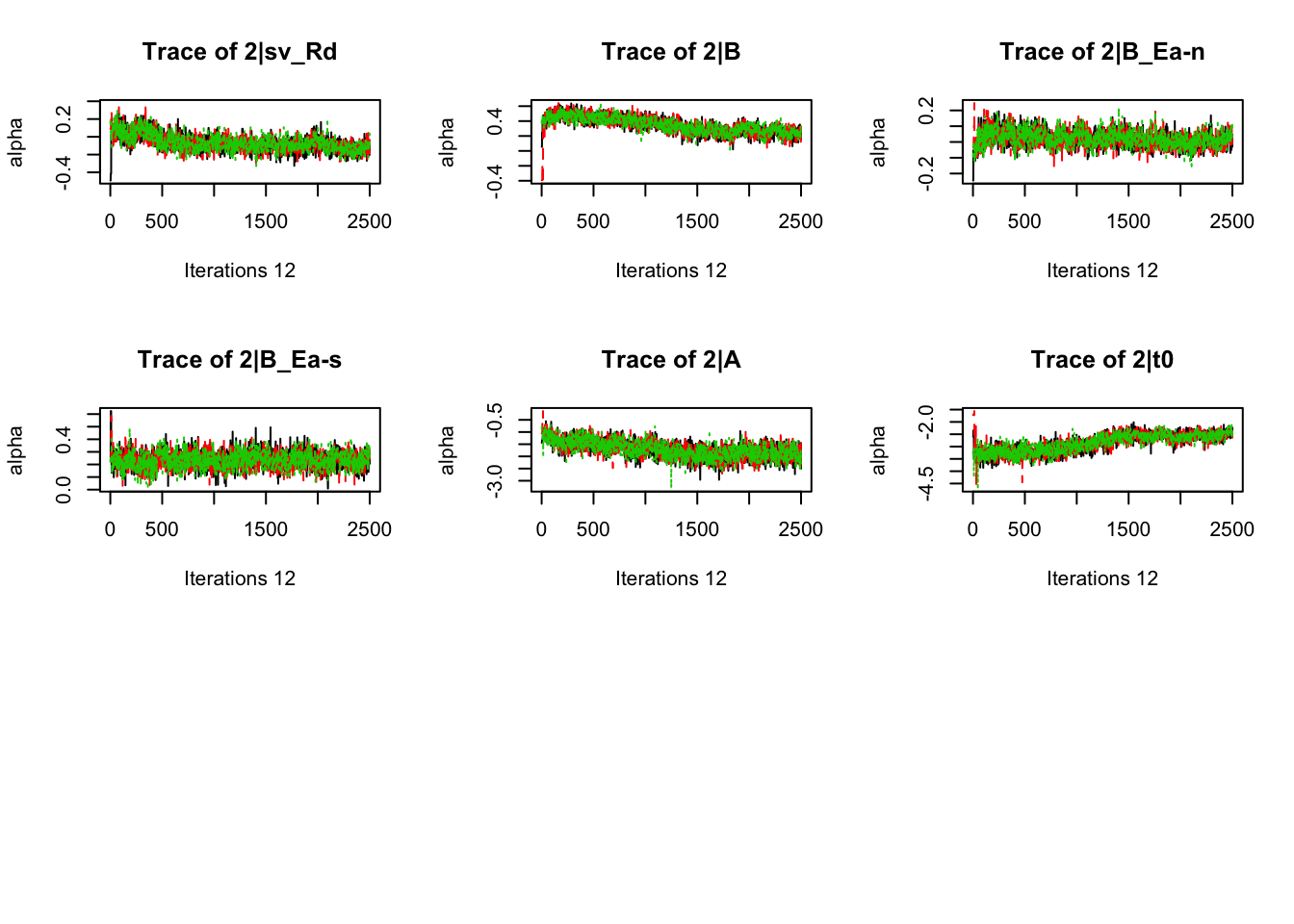
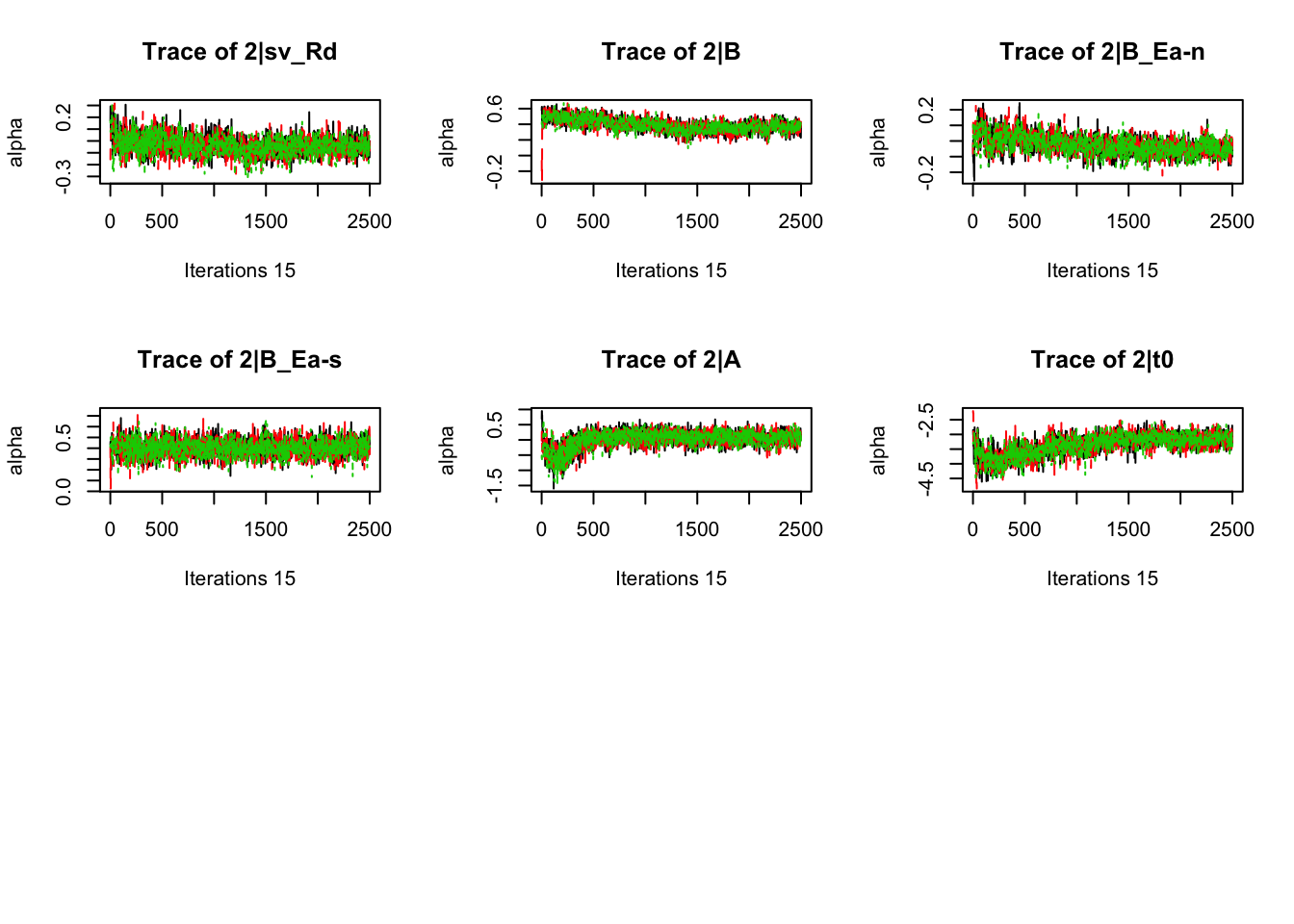
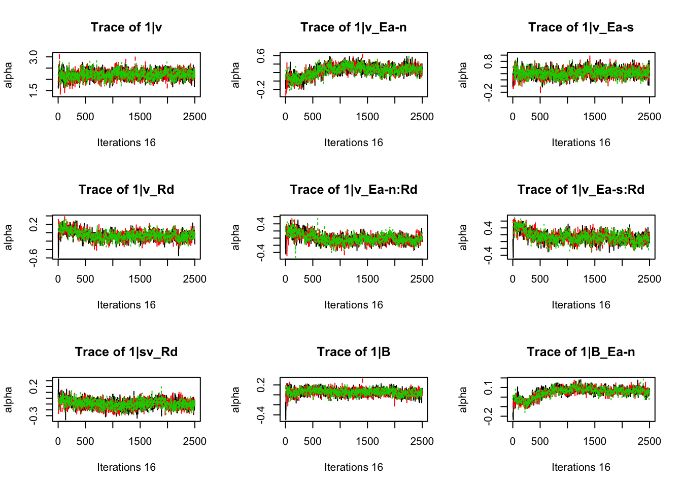
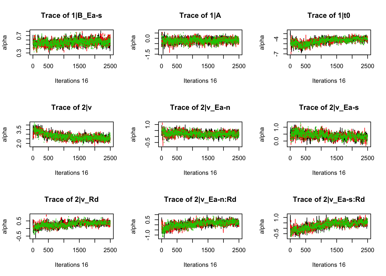
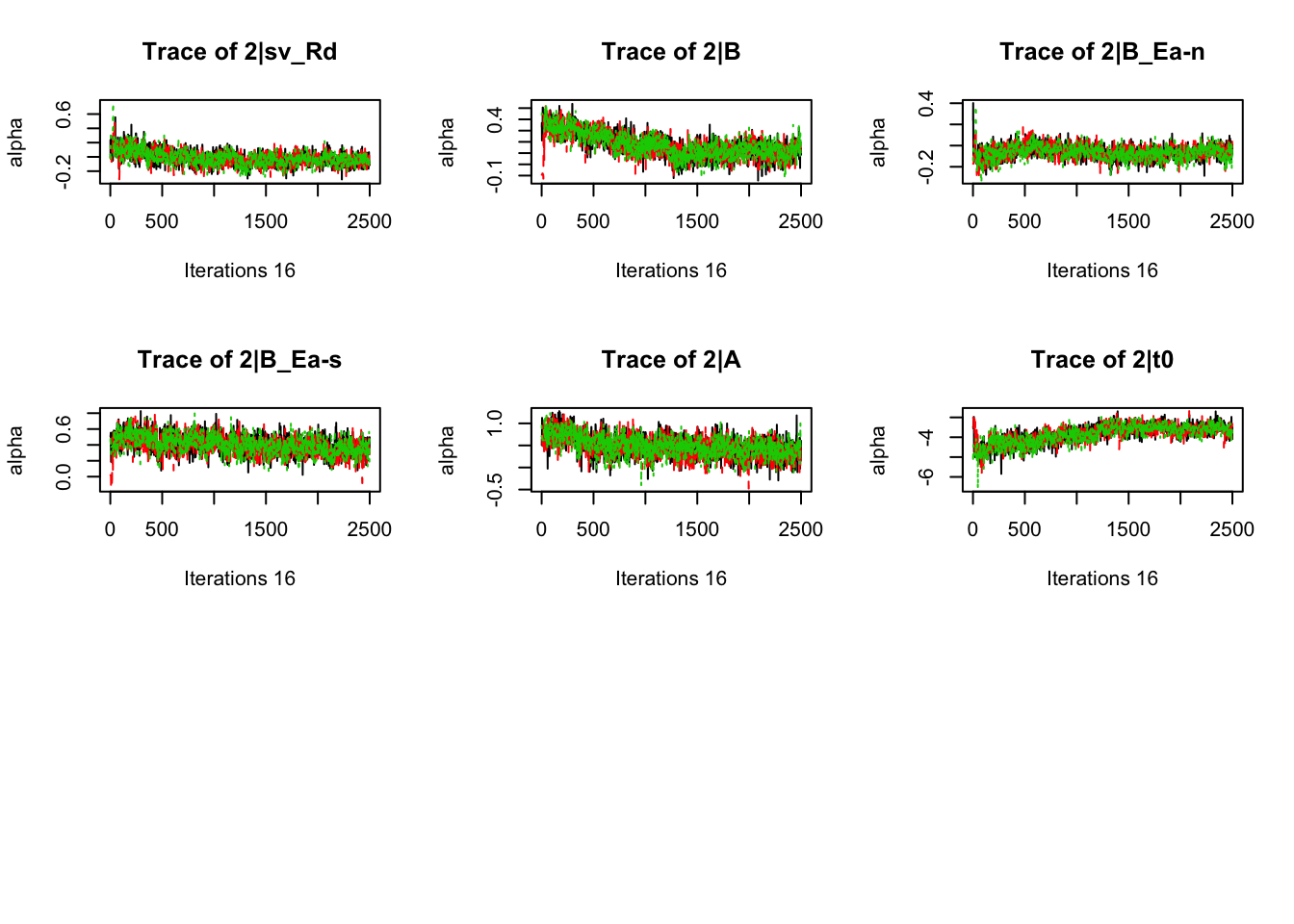
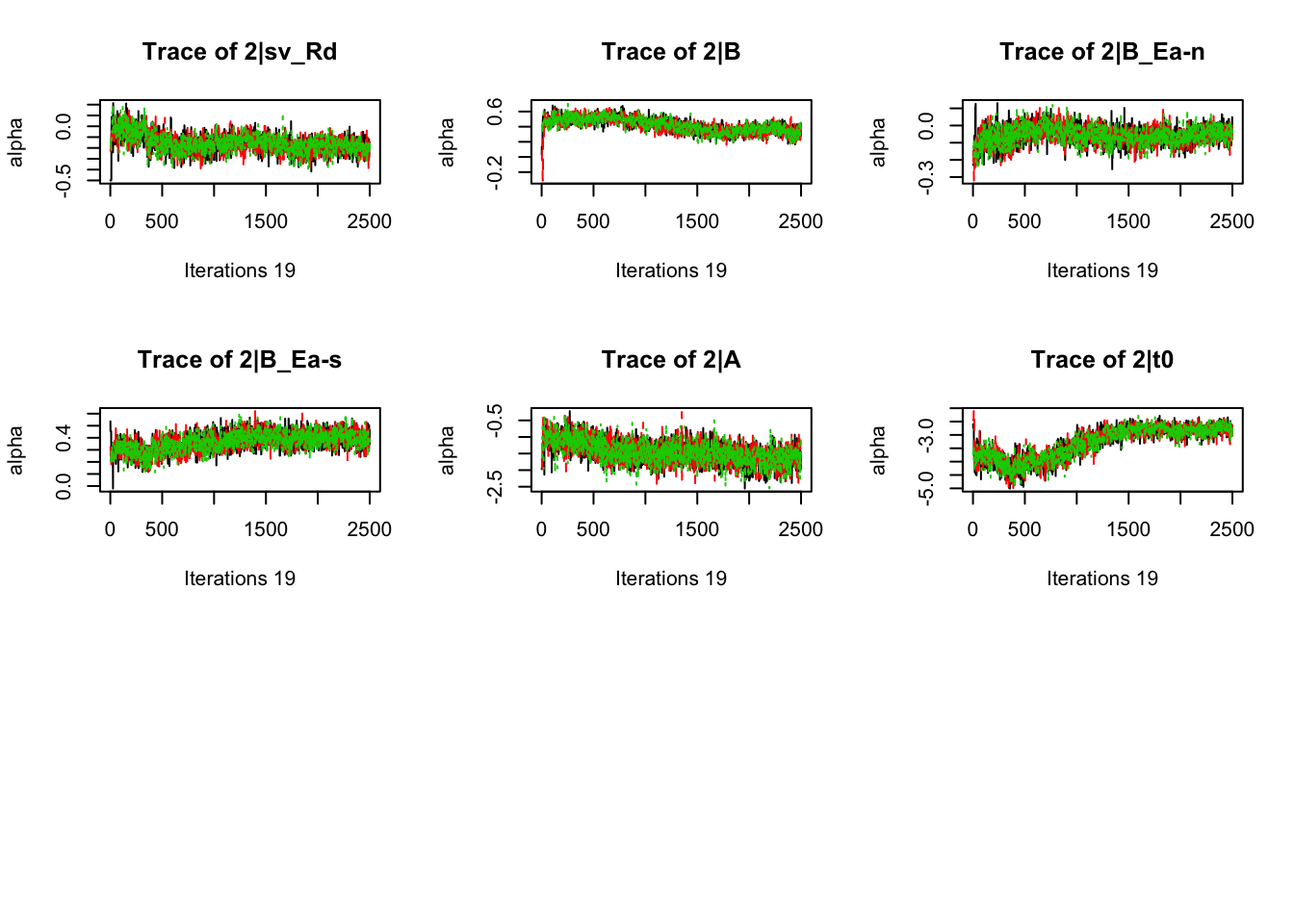
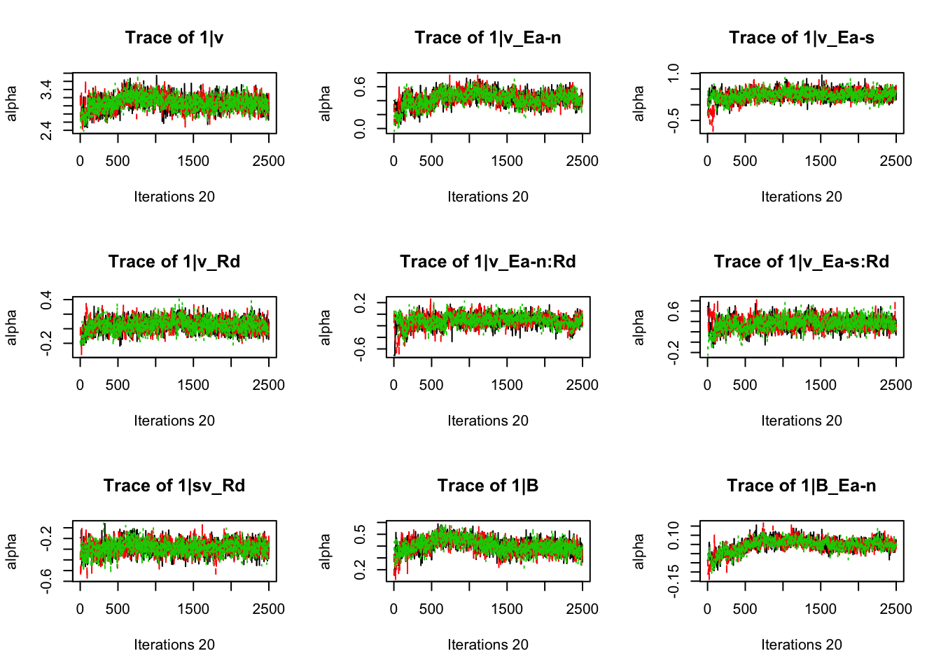
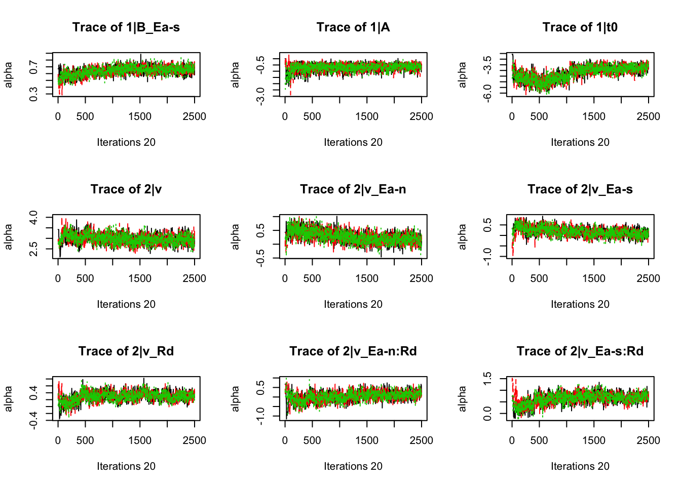
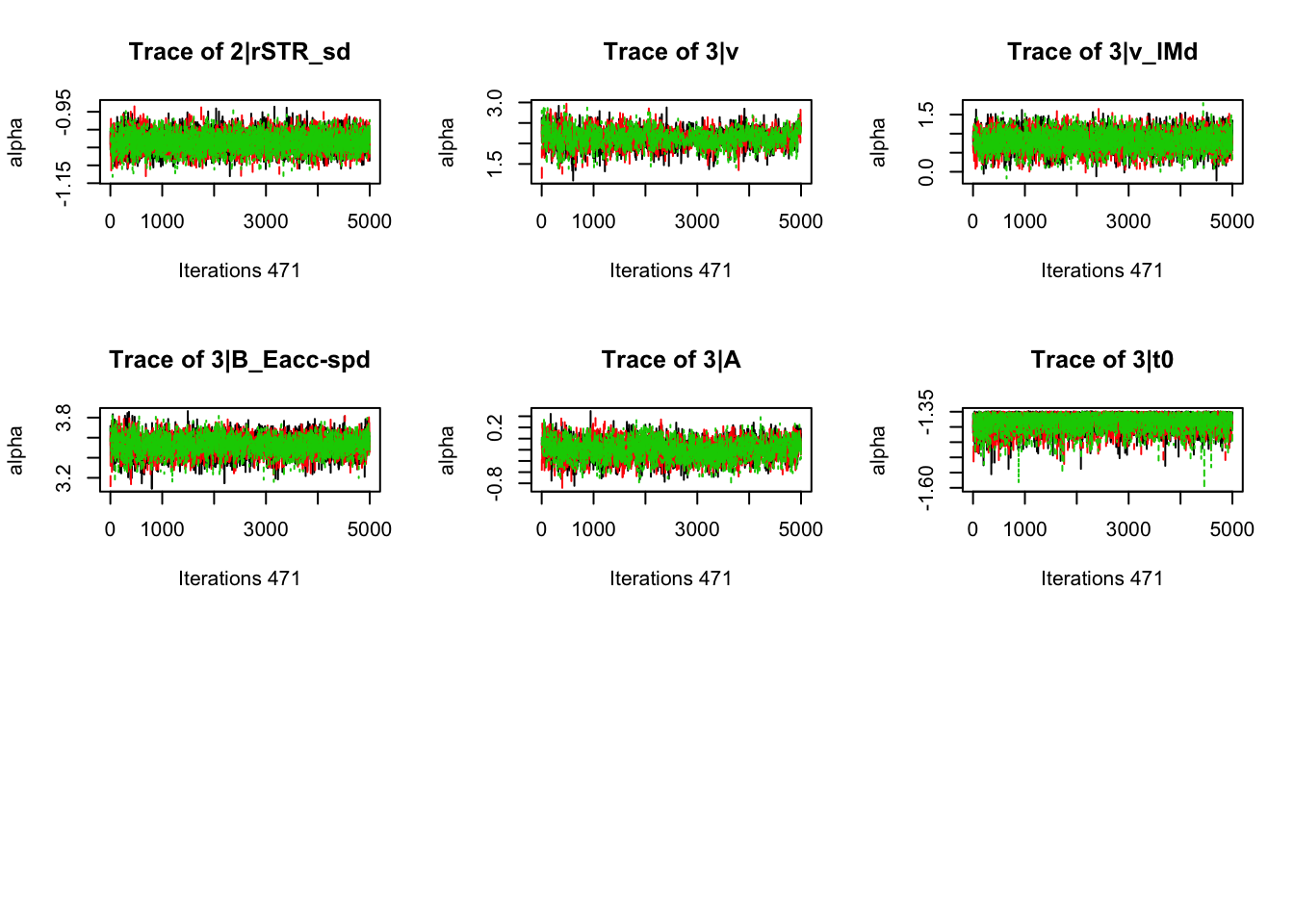
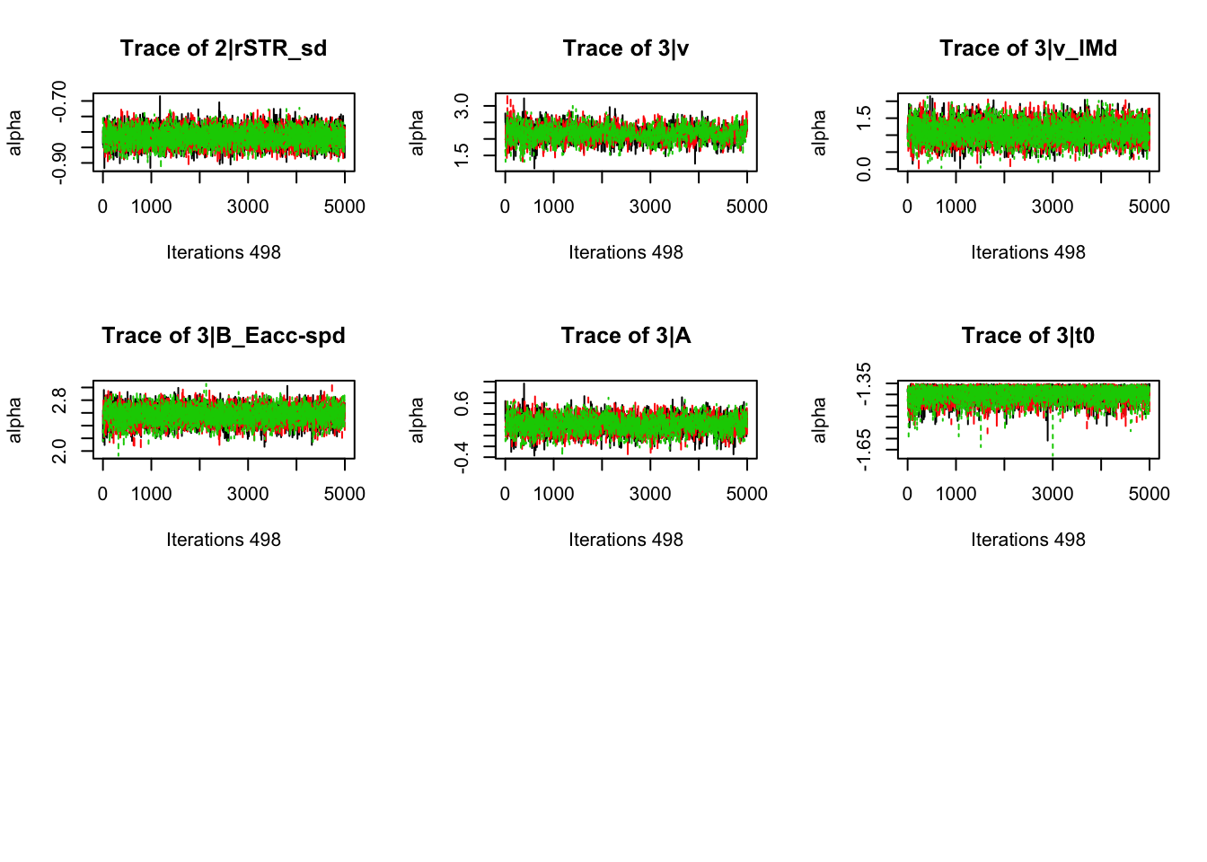
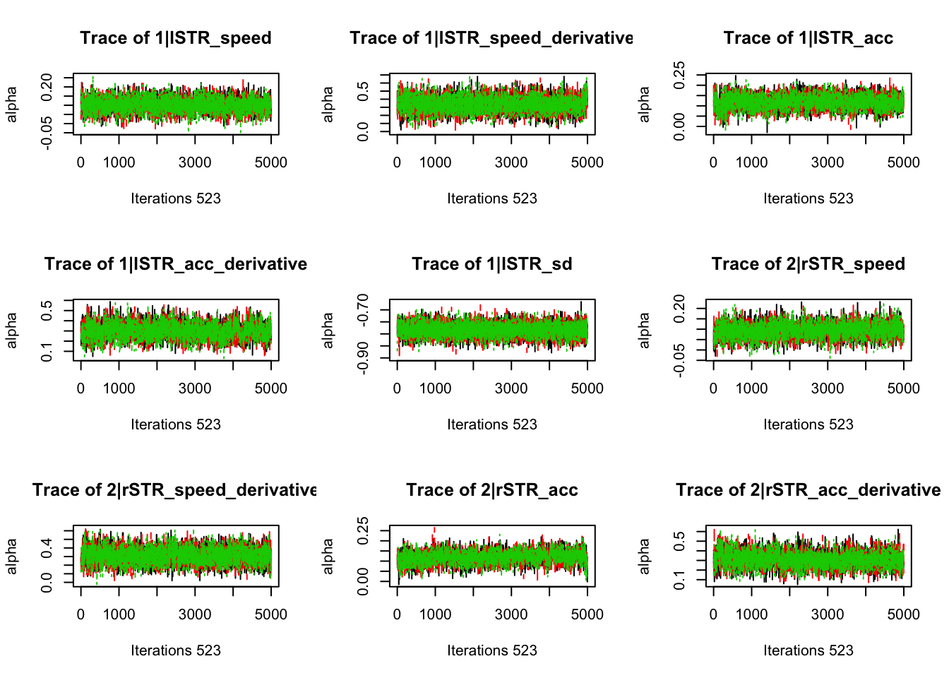
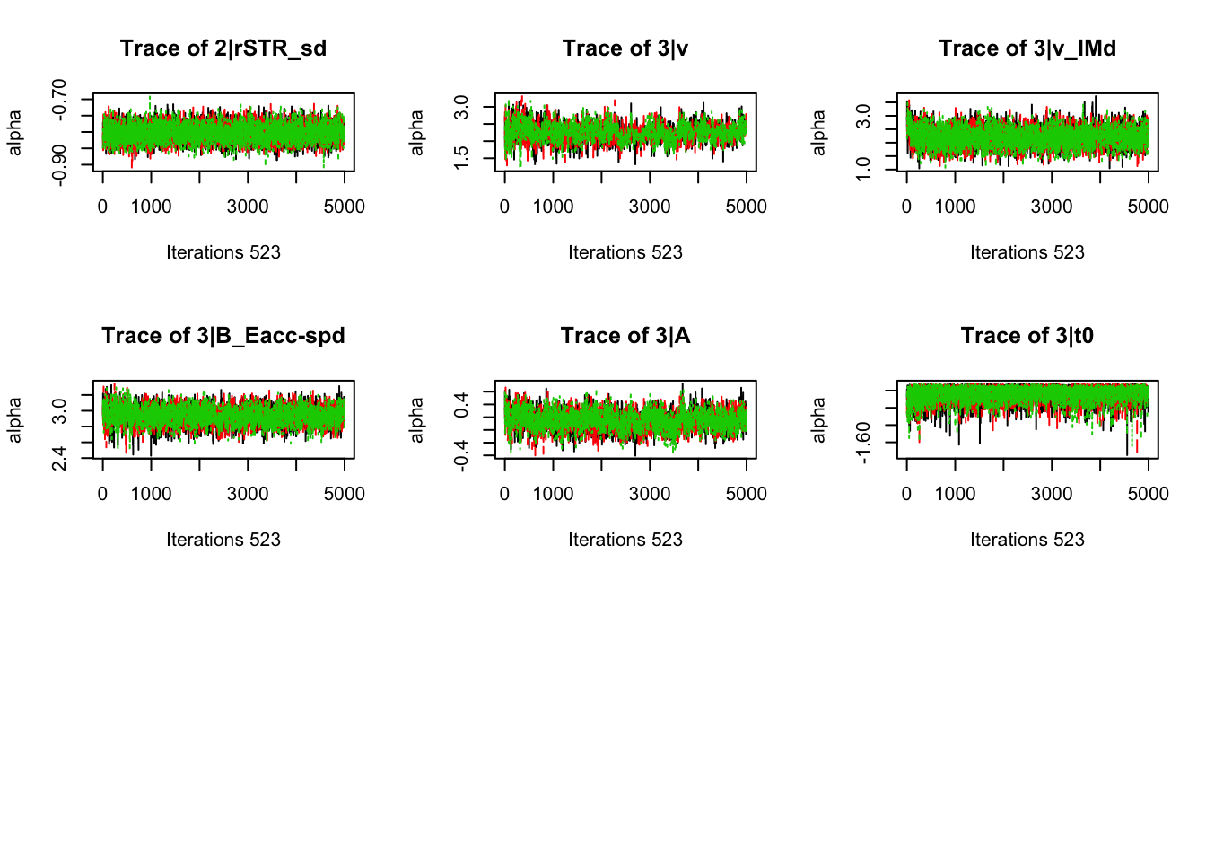
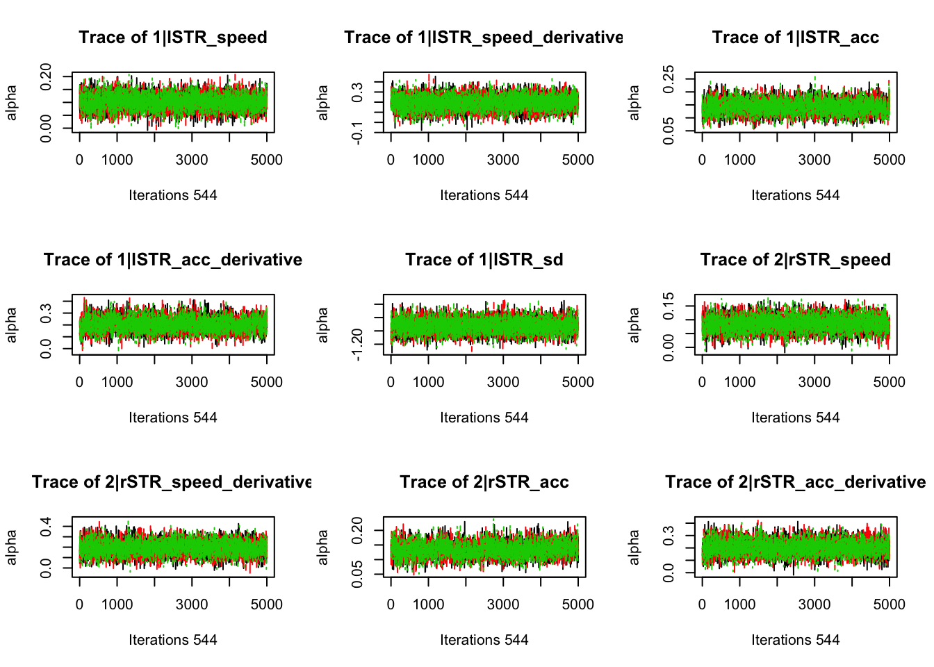
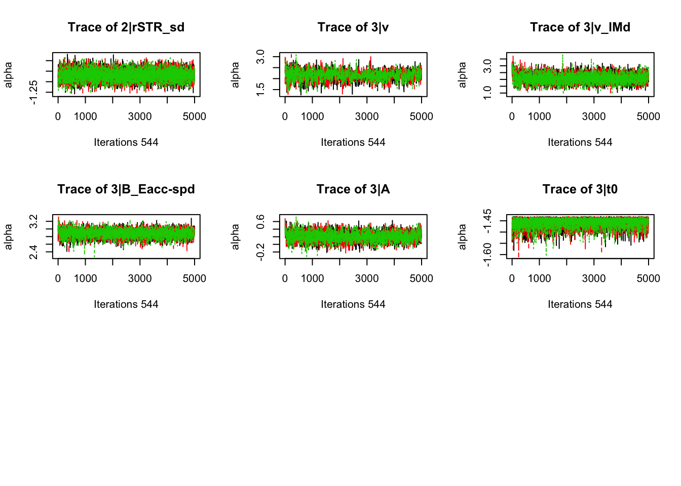
plot_chains(samples)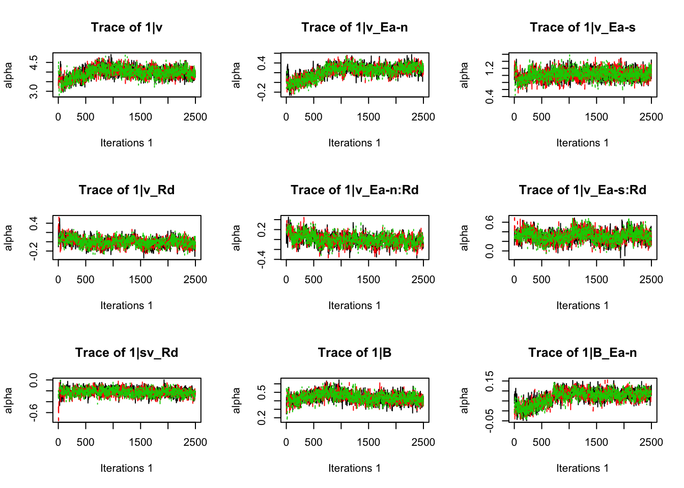
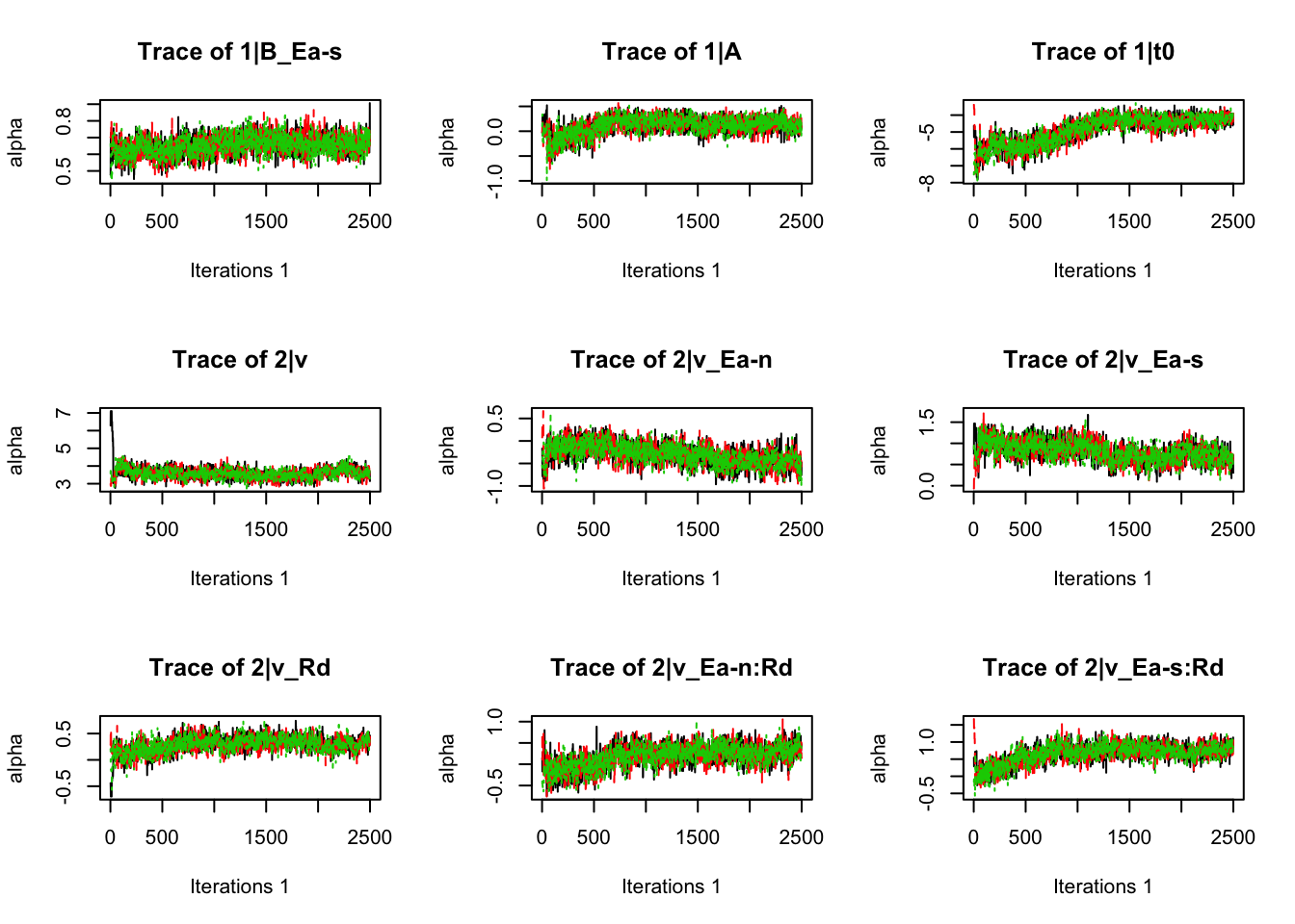
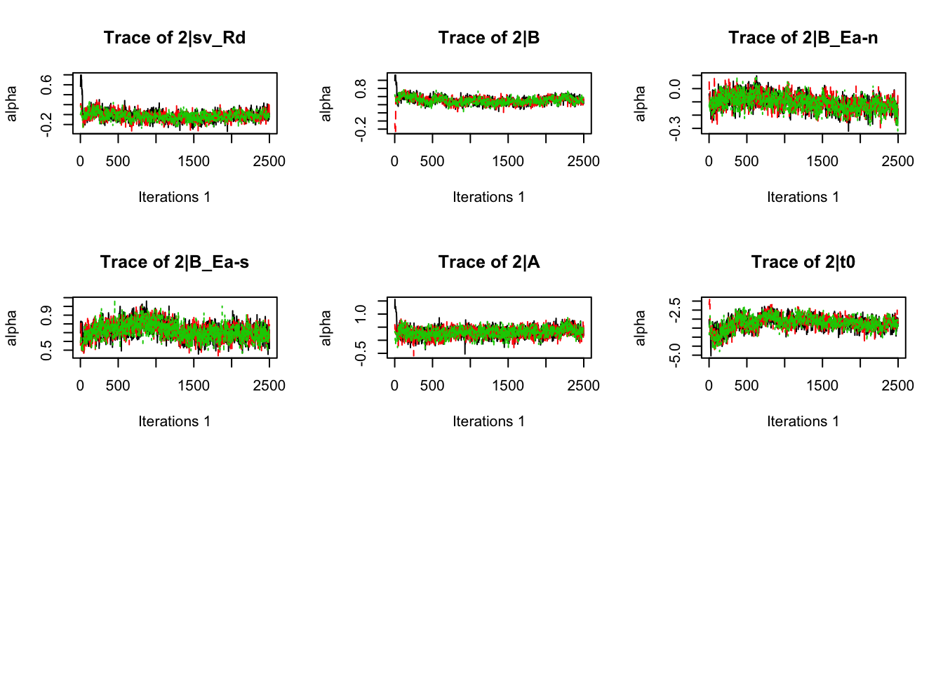
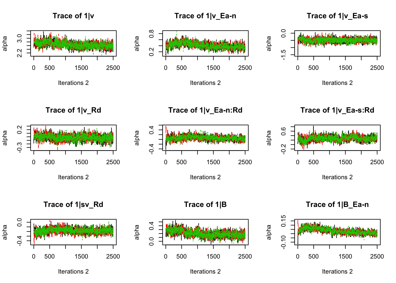
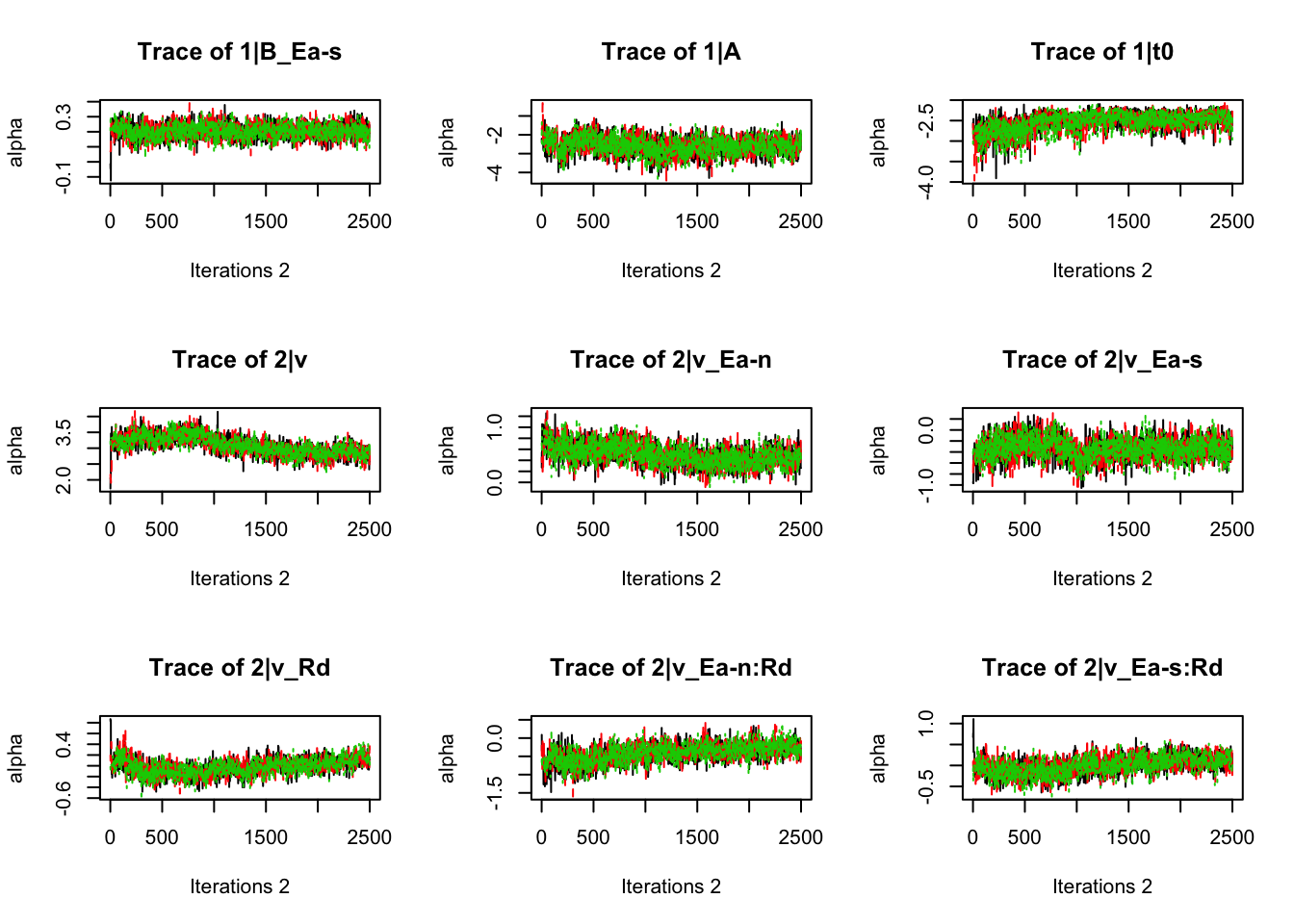
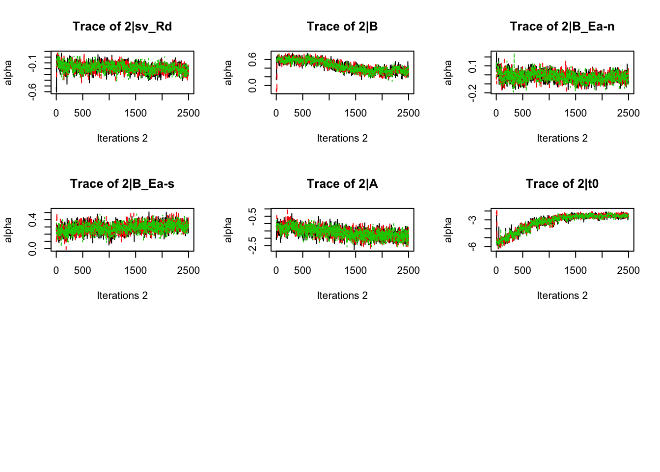
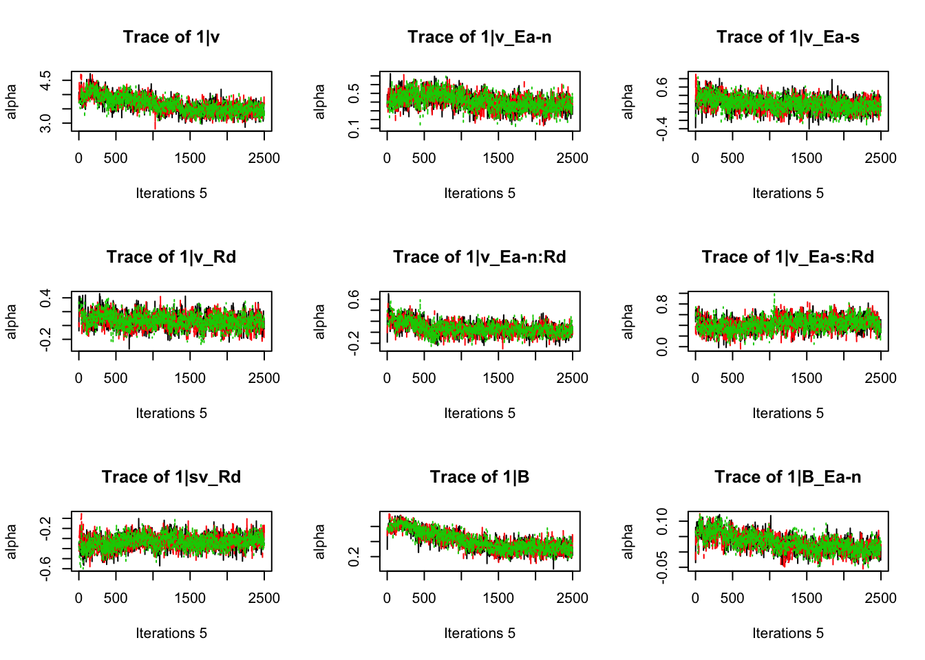
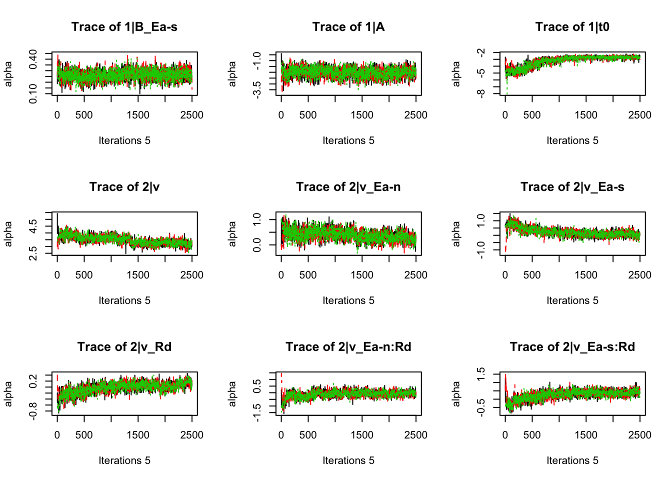
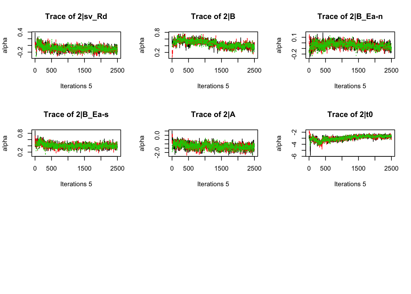
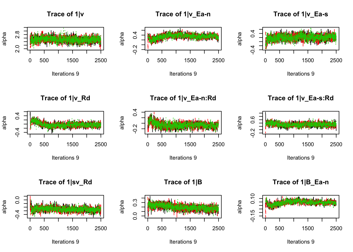
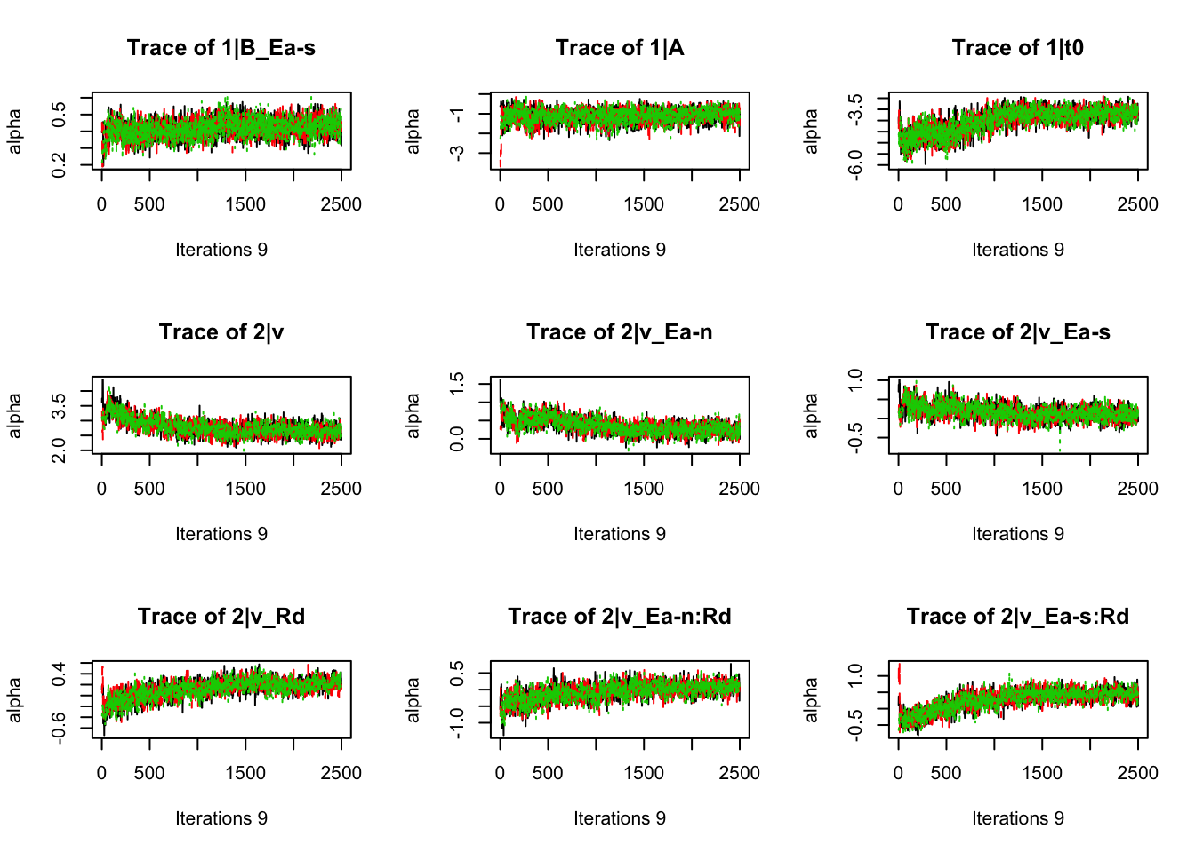
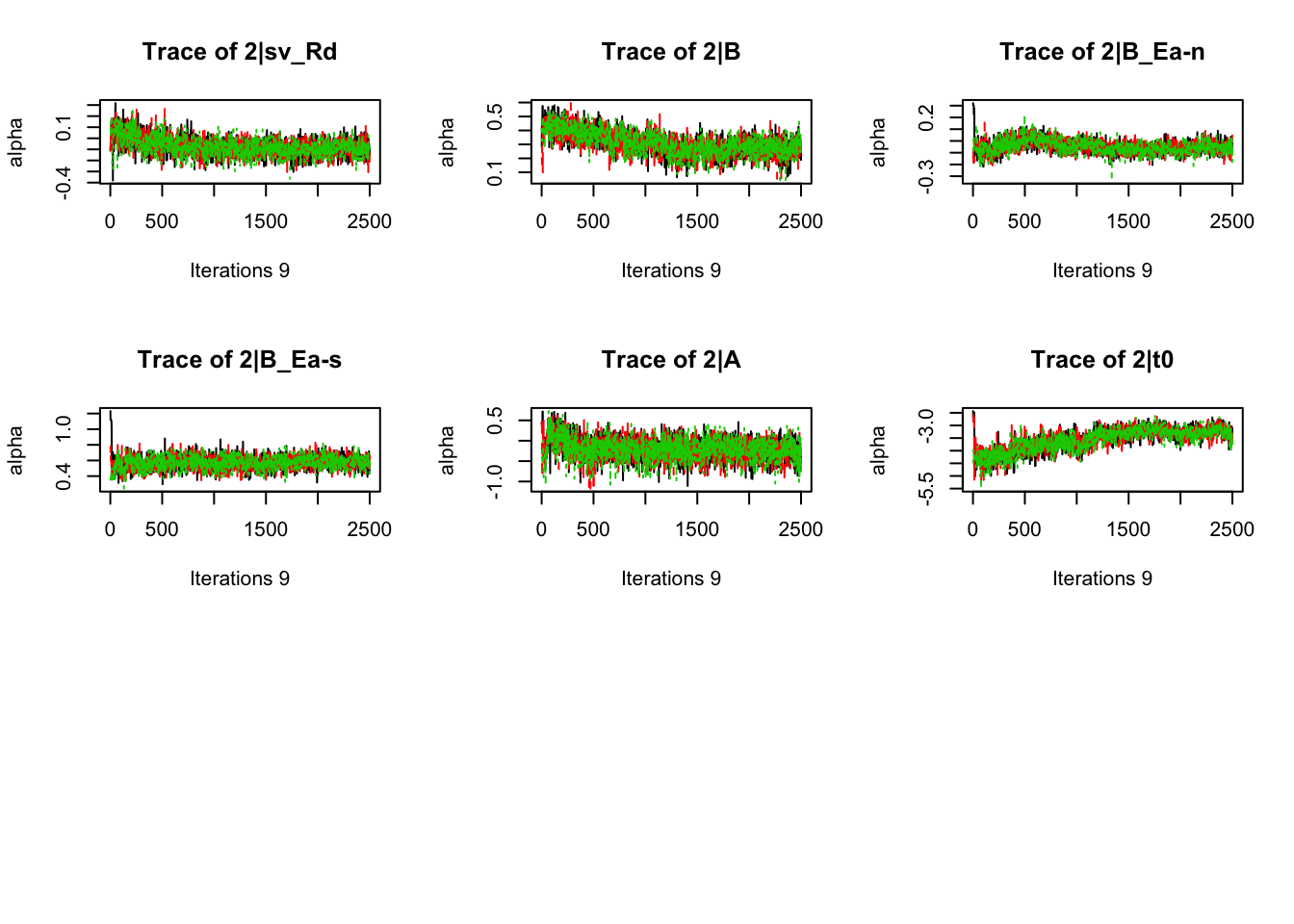
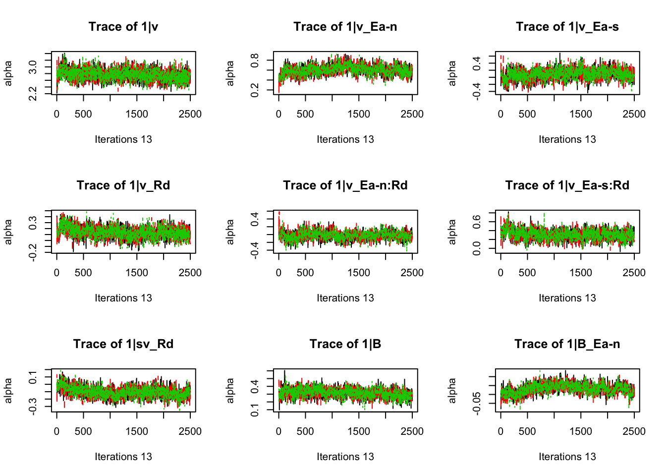
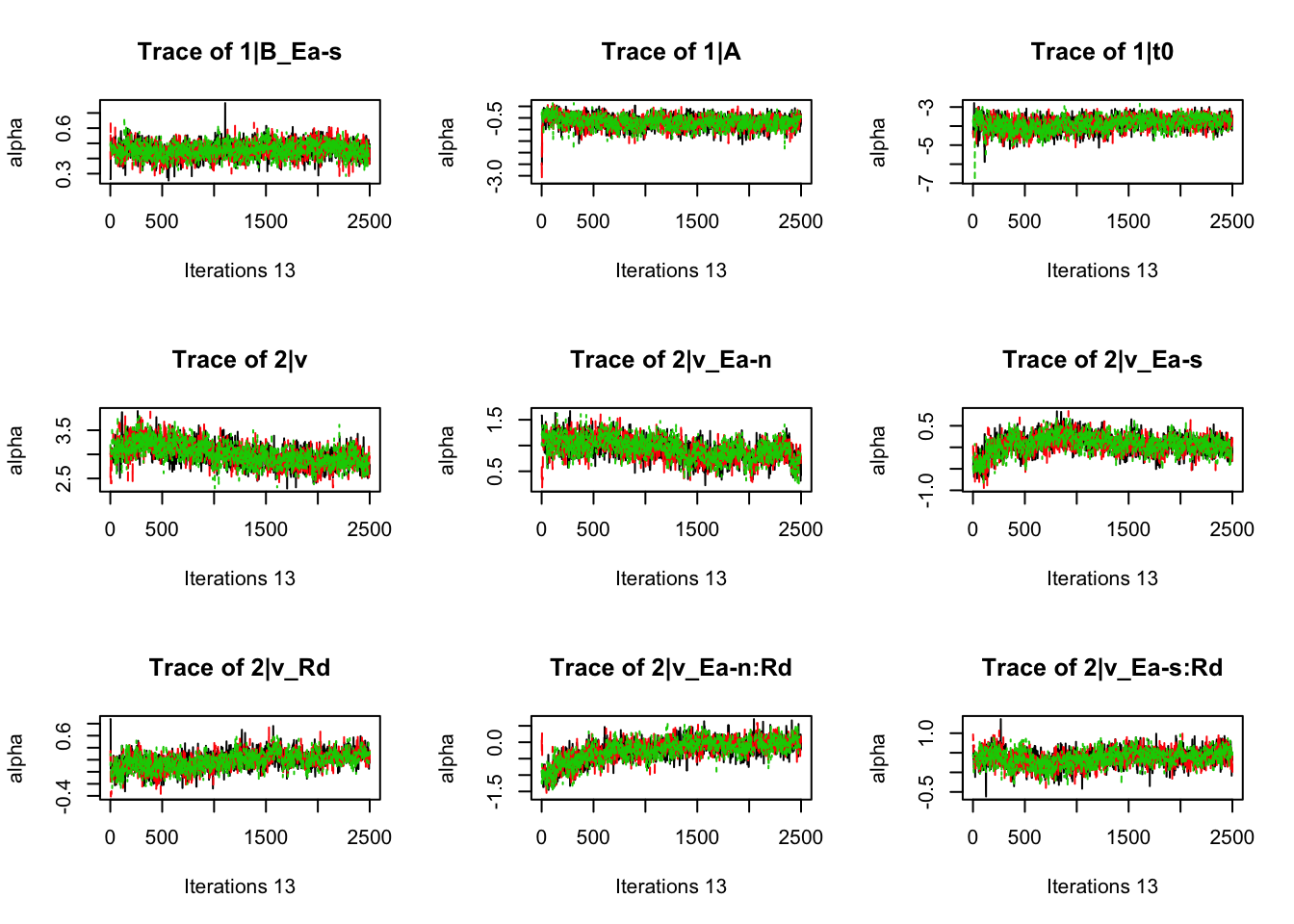
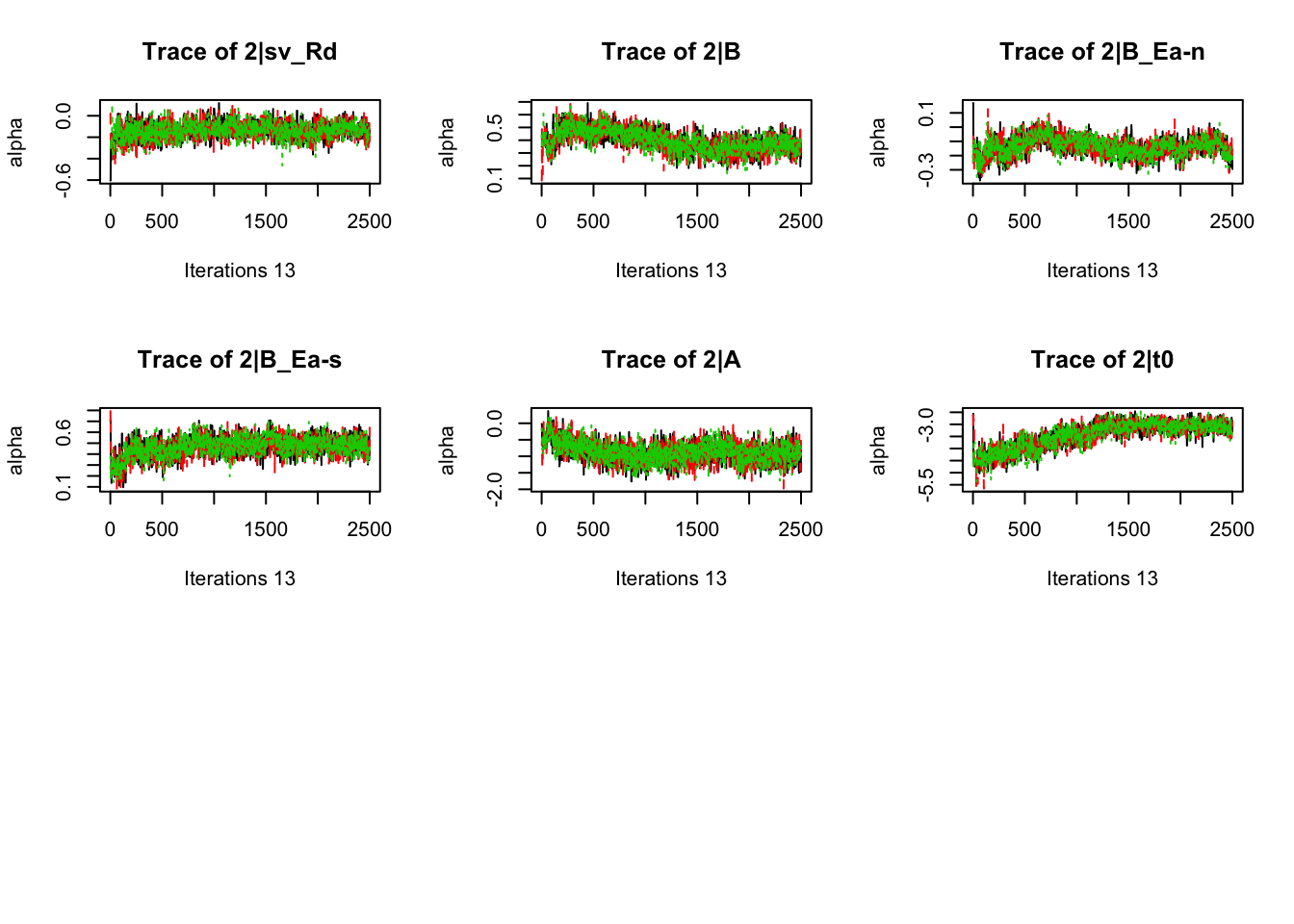
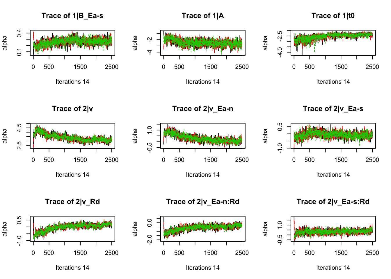
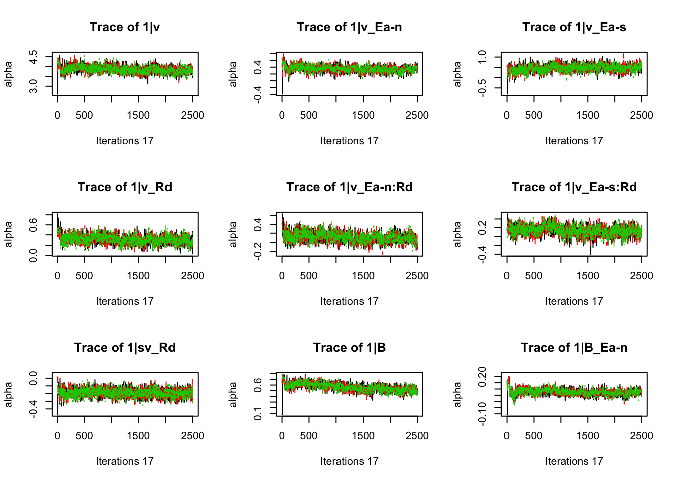
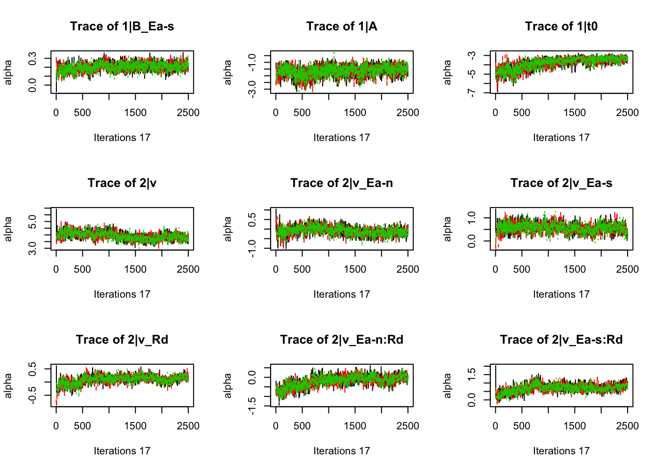
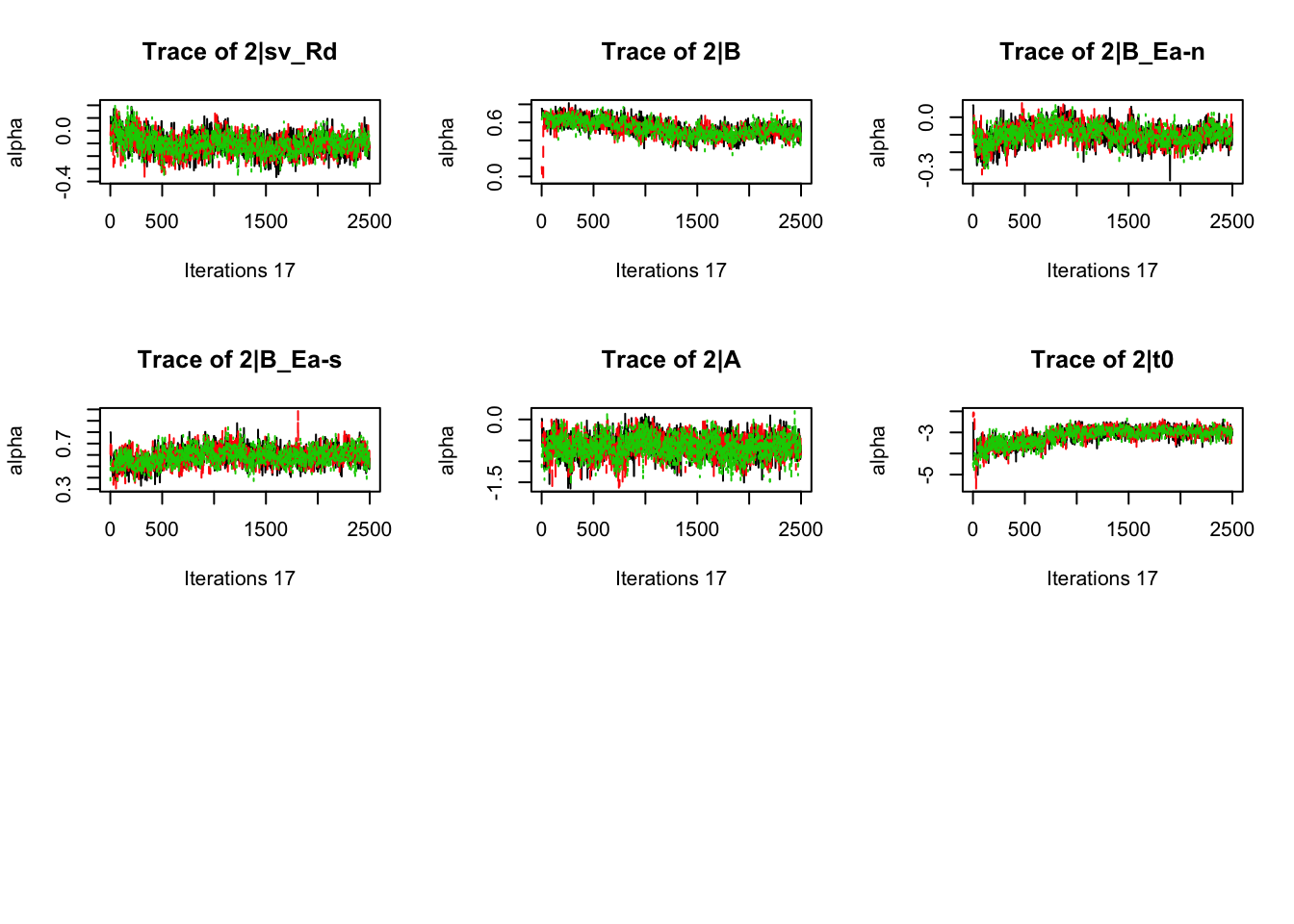
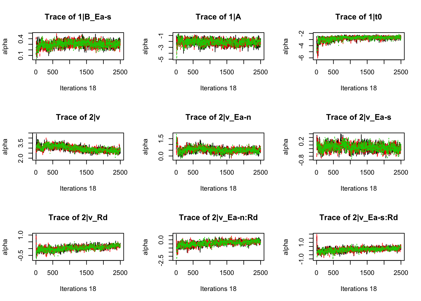
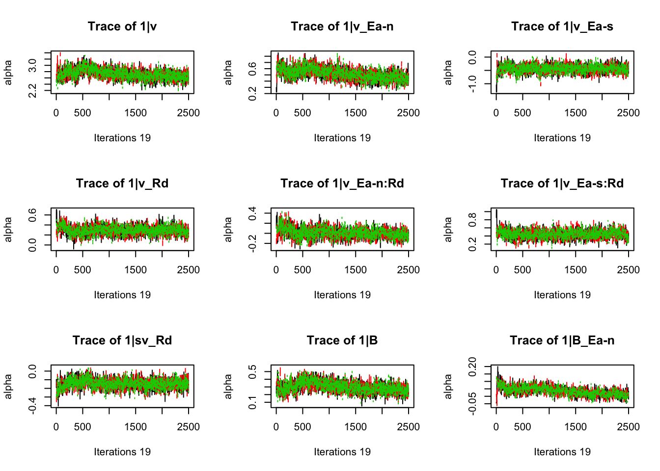
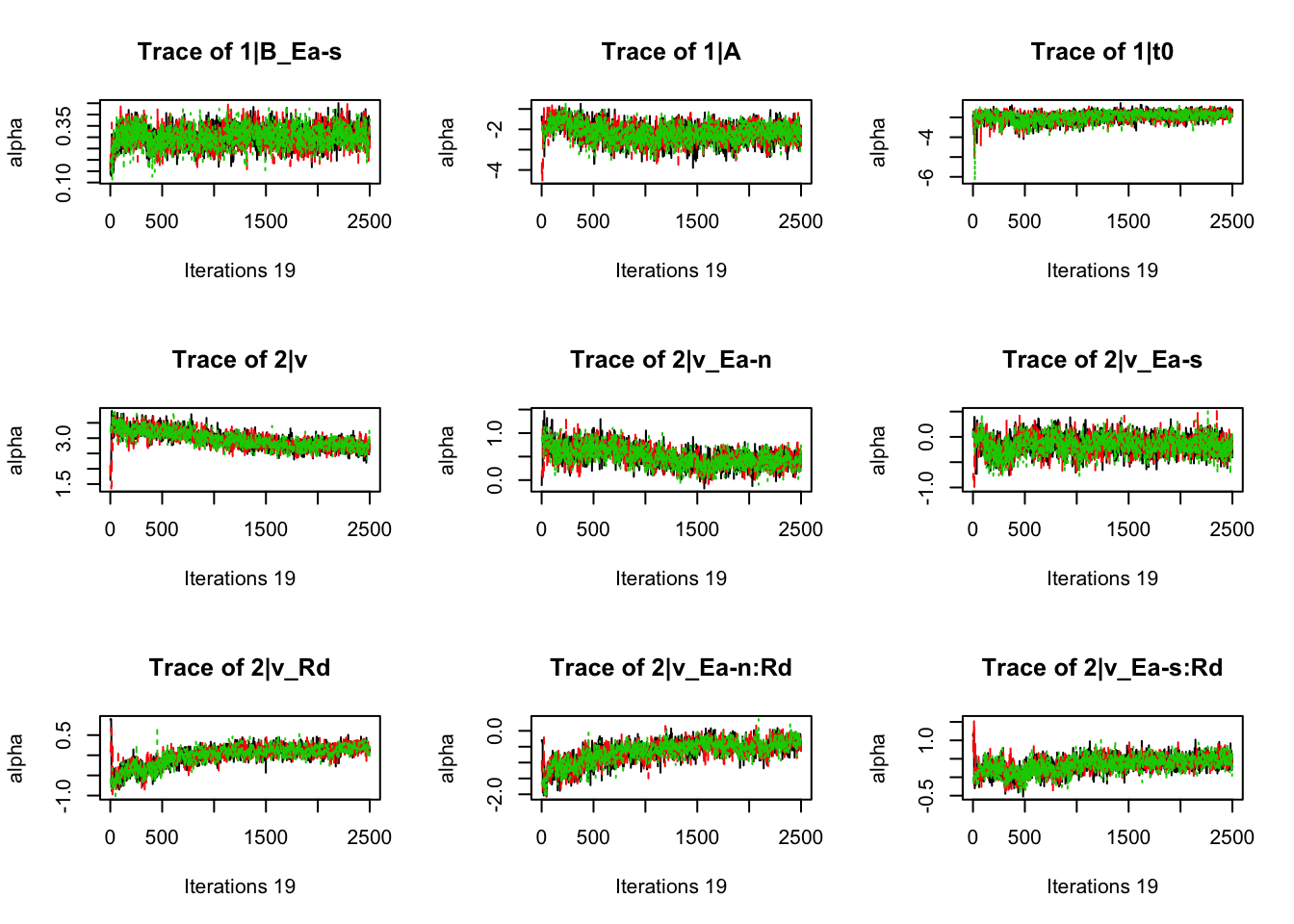
gd_pmwg(samples)## 13 4 8 14 9 10 19 3 11 7 5 18 12 2 1 17 6
## 1.00 1.00 1.01 1.01 1.01 1.01 1.01 1.01 1.01 1.01 1.01 1.01 1.01 1.01 1.01 1.01 1.01
## 16 15 20
## 1.01 1.01 1.01There’s still a bit of movement in the sample stage, so we won’t use the first 1000 samples in subsequent steps.
8.3.1.3 Analyse Fit
For analysis, we always want to check the fit. For the joint model however, it is important to run separate graphical functions for each component. We show this below.Post_predict now outputs a list, with every list entry being one component of the model.
ppJoint <- post_predict(samples,n_cores=1, filter = "sample", subfilter = 1000)
plot_fit(dat1,ppJoint[[1]],layout=c(2,3))
plot_fit(dat2,ppJoint[[2]],layout=c(2,3))
So our model fits well for out of scanner, as demonstrated earlier, but not so great in scanner. In future steps, we may have to adjust our model for the different components.
Further, because the key area of interest is in the covariance matrix at the group level, we need to get these samples to make the all important joint model inference. Let’s have a look how these look.
samples_merged <- merge_samples(samples)
library(corrplot)
median_corrs <- cov2cor(apply(samples_merged$samples$theta_var, 1:2, median))
corrplot(median_corrs)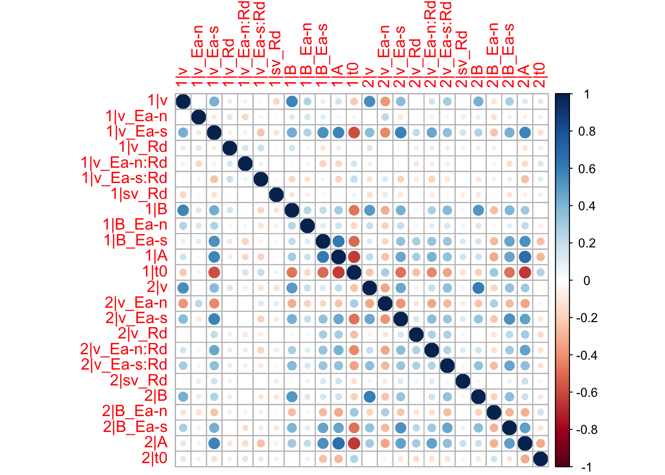
We can for example see that the drift rate and threshold parameters correlate between sessions, particularly for the speed emphasis. From the drift rates we can for example conclude that participants who were good at task 1, were also good at task 2. And from the thresholds we can conclude that participants used the same strategy between the tasks.
8.3.2 Behavioural x Neural Data
For our second example, we show a joint model of neural data and behavioural data. The data was taken from van Maanen et al. (2011) where the authors again used a speed-accuracy tradeoff manipulation for a random dot motion task. The authors were interested in changes to latent behavioural mechanisms (like threshold changes) and changes to neural activation (mainly in the striatum which is thought to modulate caution). Here, we model the behavioural data as before, and model the contrasts in the fMRI data using a regression model. The key question here is one that is highly interesting to cognitive neuroscience, and any researchers in functional imaging studies; do latent parameters correspond to activation changes in the brain?
Let’s first load in the data. For the fMRI part we need both the activation and a design matrix where the bold response is deconvolved. Here we’ve already regressed out nuisance parameters that account for, for example physiological noise. For more info on that, come to us later!
rm(list=ls())
library(mvtnorm)
source("emc/emc.R")
source("models/fMRI/Normal/normal.R")
source("models/RACE/LBA/lbaB.R")

# Load in the data
load("Data/VM2011/fmri_dm_VM2011.RData")
load("Data/VM2011/fmri_data_VM2011.RData")
load("Data/VM2011/behav_data_VM2011.RData")

behav_data <- behav_data[,c("subject", "cond", "stimulus", "response", "RT")]
colnames(behav_data) <- c('subjects', 'E', 'S', 'R', 'rt')
behav_data$R<- as.factor(behav_data$R)
behav_data$S<- as.factor(behav_data$S)
behav_data$subjects<- as.factor(behav_data$subjects)
8.3.3 Neural Model
Now, let’s introduce the model of the neural component. This can simple be done by inputting the data and the design matrix in the make_design_fmri function. Here we only look at the left and right striatum activation in a region of interest based analysis.
# subset data to only have one roi
data_lSTR <- fmri_data[, c("lSTR", "subjects")]
data_rSTR <- fmri_data[, c("rSTR", "subjects")]
design_lSTR <- make_design_fmri(design_matrix = fmri_dm, data = data_lSTR, model = normal)
design_rSTR <- make_design_fmri(design_matrix = fmri_dm, data = data_rSTR, model = normal)
8.3.3.1 Combine Designs
Once we set up the design for the behavioural component, we can combine the designs as before so that we are ready to sample.
Emat <- matrix(c(-1,1),ncol=1)
dimnames(Emat) <- list(NULL,"acc-spd")     # estimate the contrast between ACC-SPD trials

# Average rate = intercept, and rate d = difference (match-mismatch) contrast
ADmat <- matrix(c(-1/2,1/2),ncol=1,dimnames=list(NULL,"d"))

design_behav <- make_design(
  Ffactors=list(subjects=levels(behav_data$subjects),S=levels(behav_data$S),E=levels(behav_data$E)),
  Rlevels=levels(behav_data$R),matchfun=function(d)d$S==d$lR,
  Clist=list(lM=ADmat,lR=ADmat,S=ADmat,E=Emat),
  Flist=list(v~lM,sv~1,B~E,A~1,t0~1),       # <-- only B affected by E
  constants=c(sv=log(1), B=log(0.05)),
  model=lbaB)
sampler <- make_samplers(list(data_lSTR, data_rSTR, behav_data), list(design_lSTR, design_rSTR, design_behav))8.3.3.2 Sample
Sampling for this model can be tricky. This problem was referred to before with EMC’s trick in estimation, where we first estimate each component individually before fitting them together. This is because some models have a tendency to dominate the estimation space, as the fMRI component does in this example. This happens because the likelihood estimate is much higher, so changes to the behavioural model may not effect the overall model as greatly. Because of this, we should sample the posterior for longer, and ensure we carry out a variety of posterior checks on convergence and stationarity.
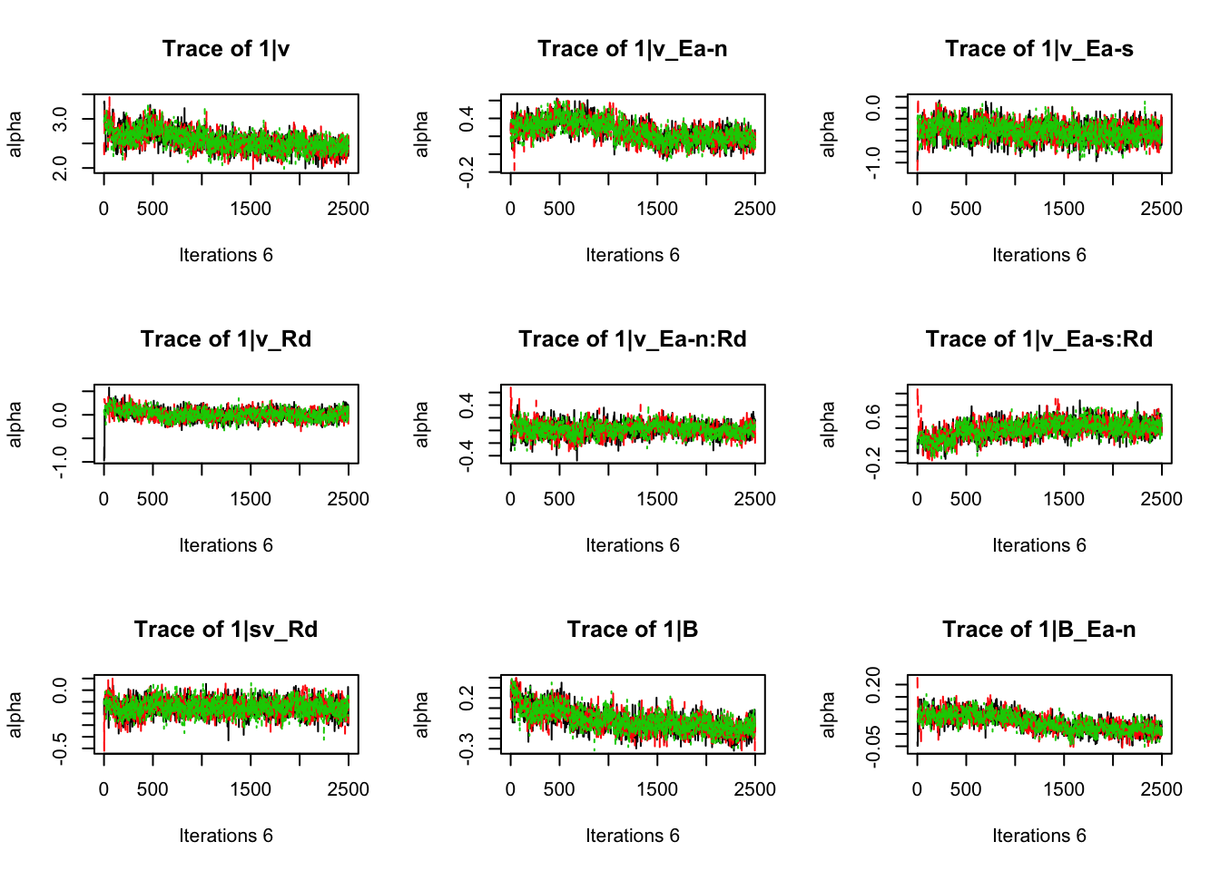
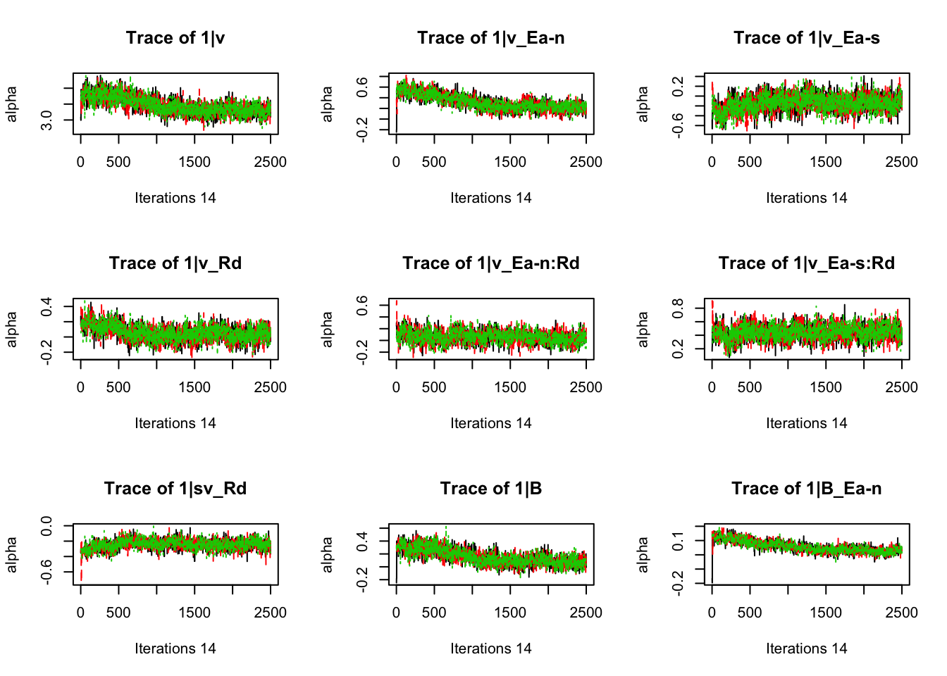
samples <- run_emc(sampler, nsample = 5000, cores_per_chain = 8, cores_for_chains = 3, verbose_run_stage = T)Let’s load in the pre-sampled data instead;
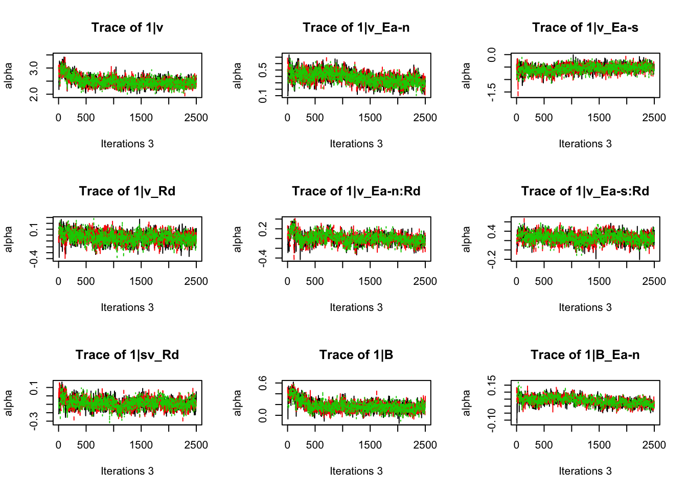
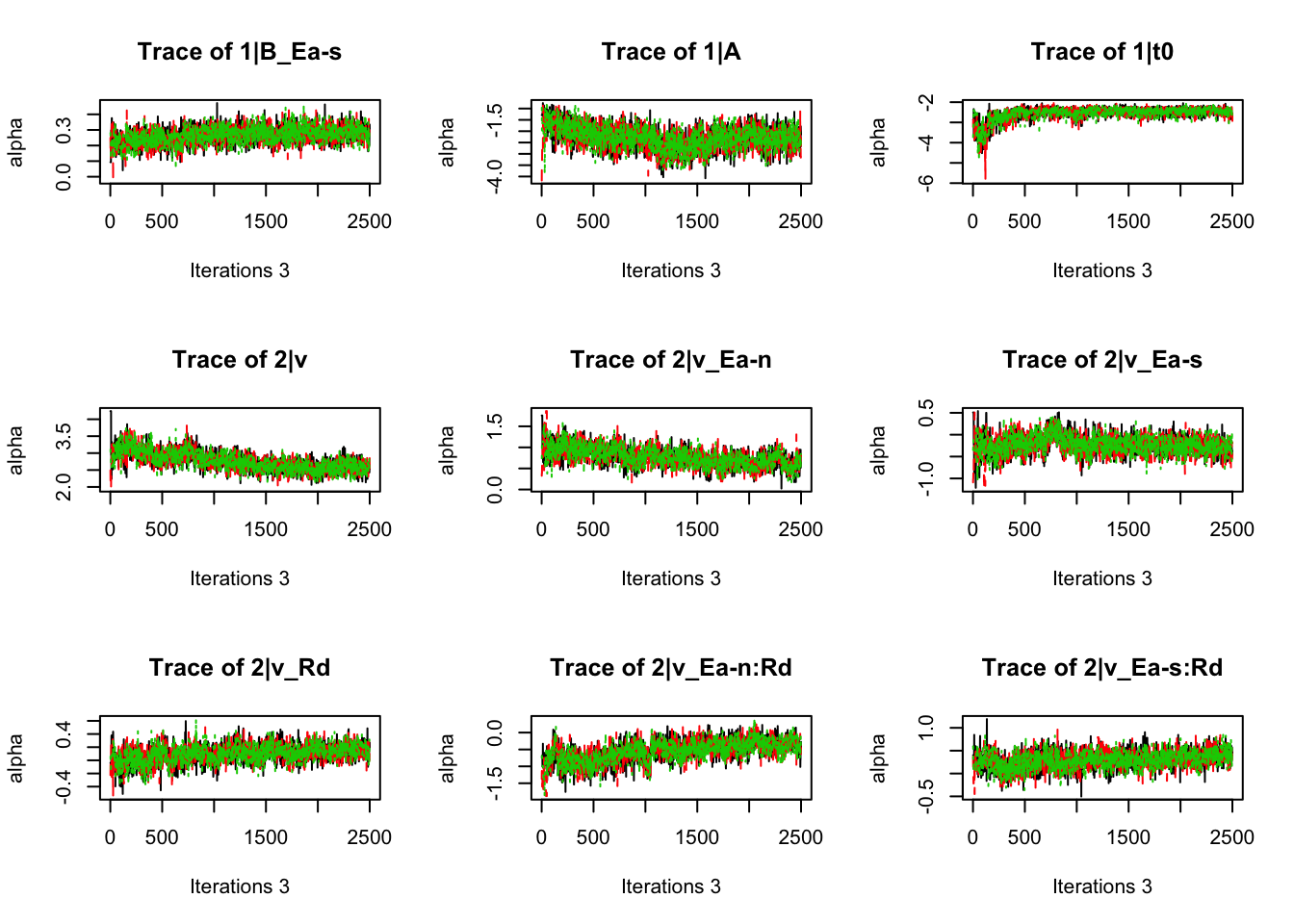
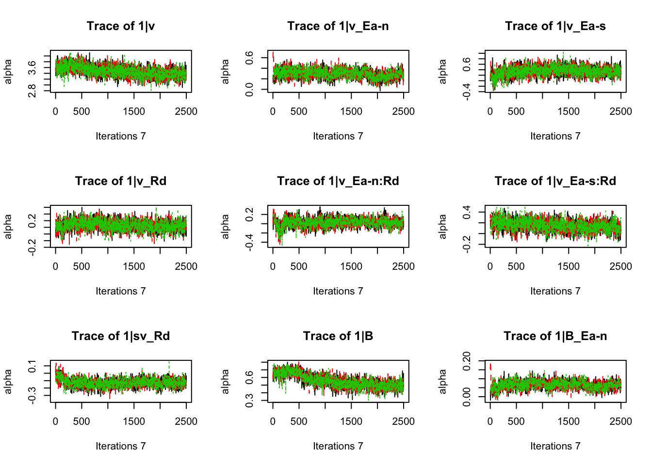
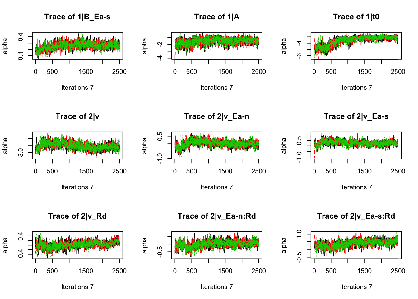
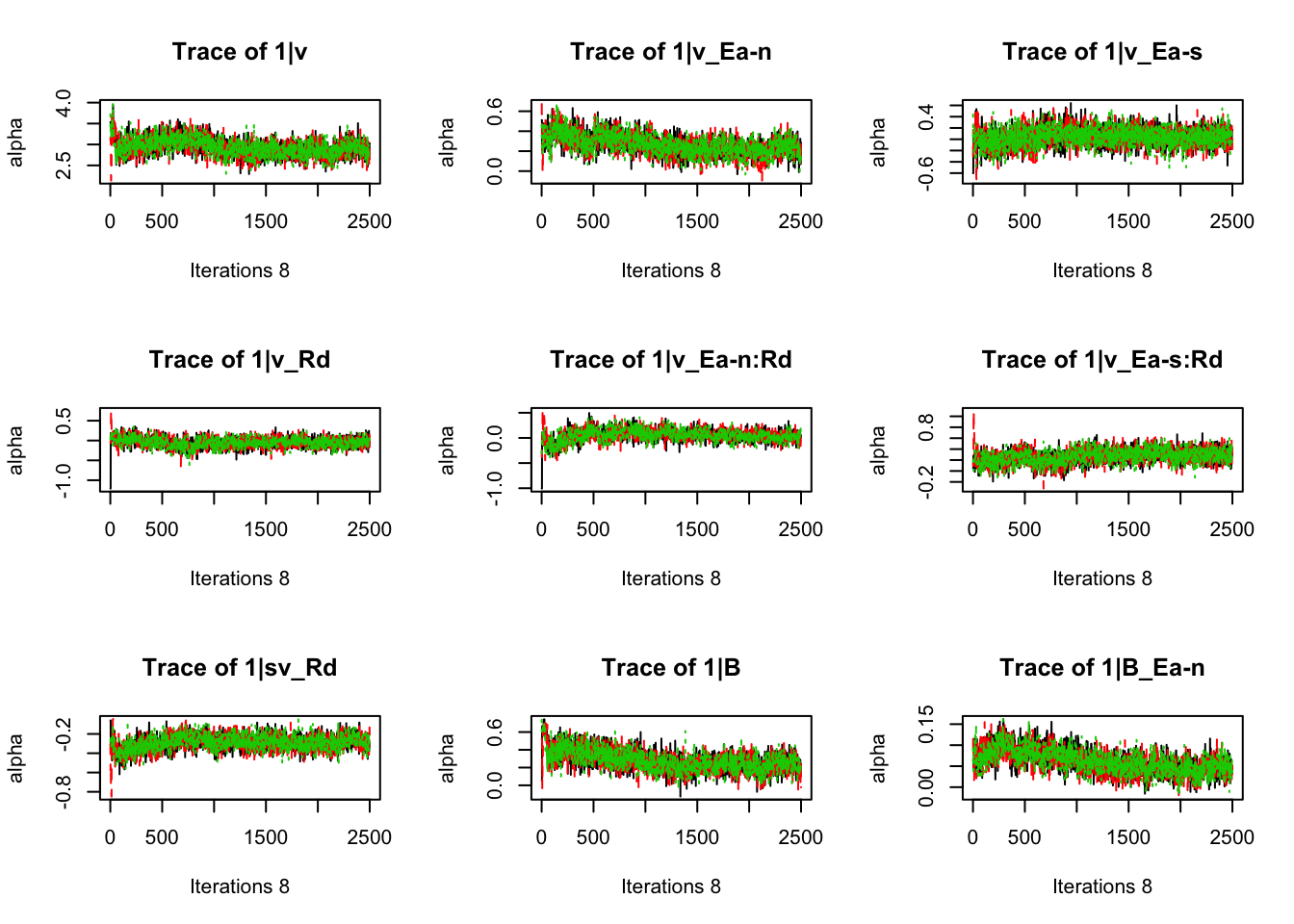
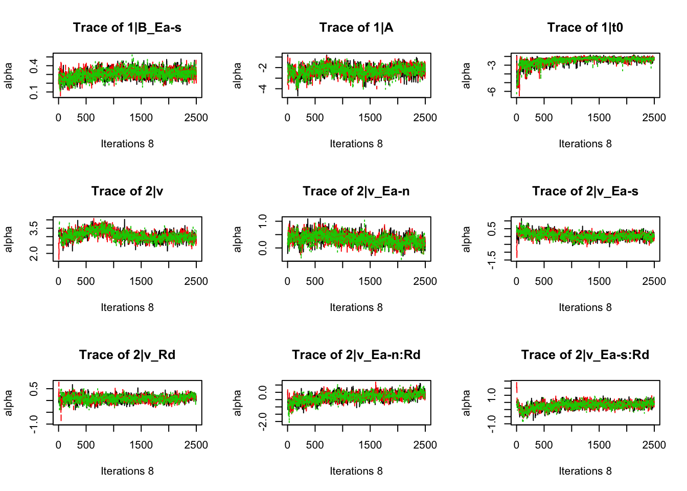
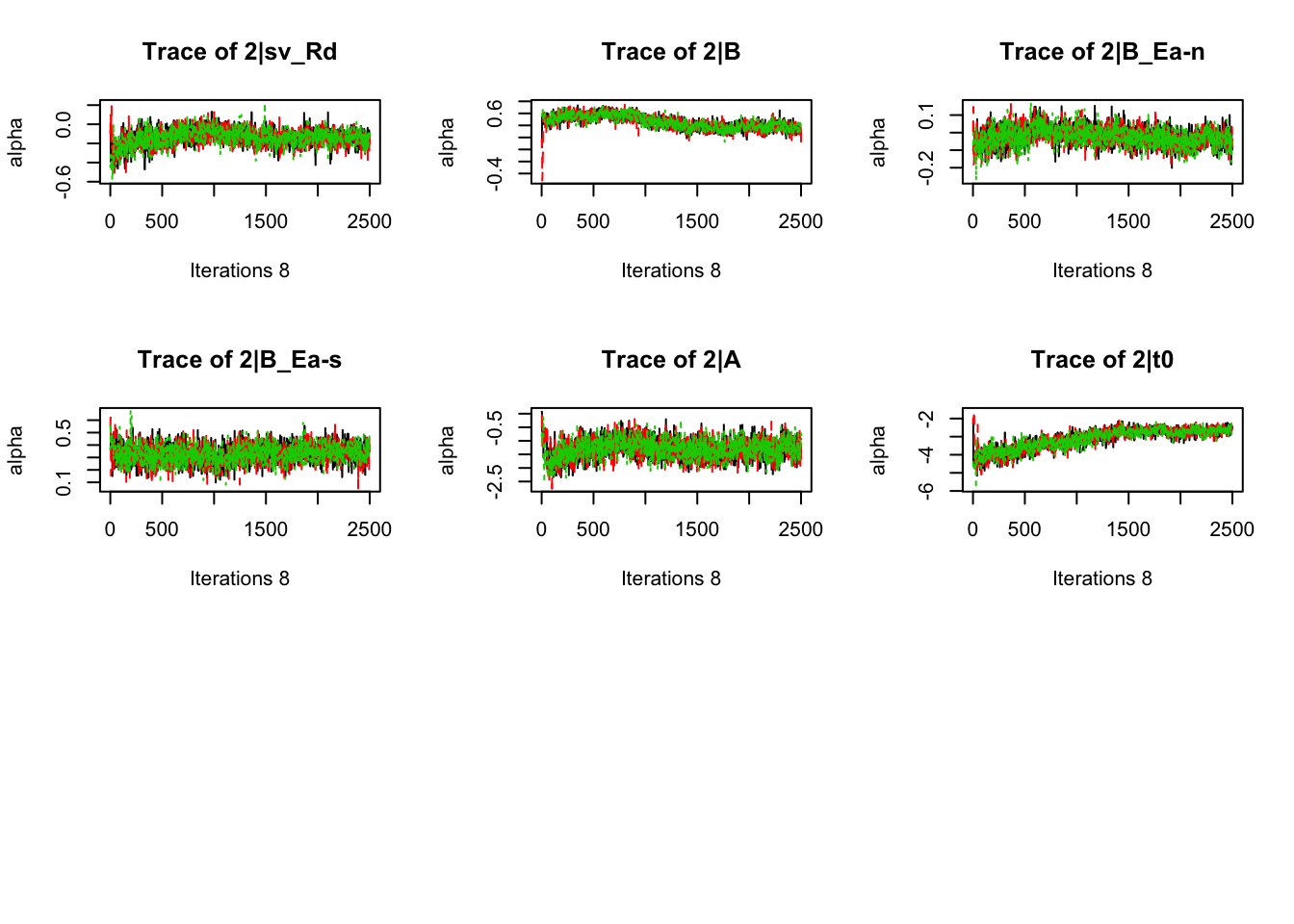
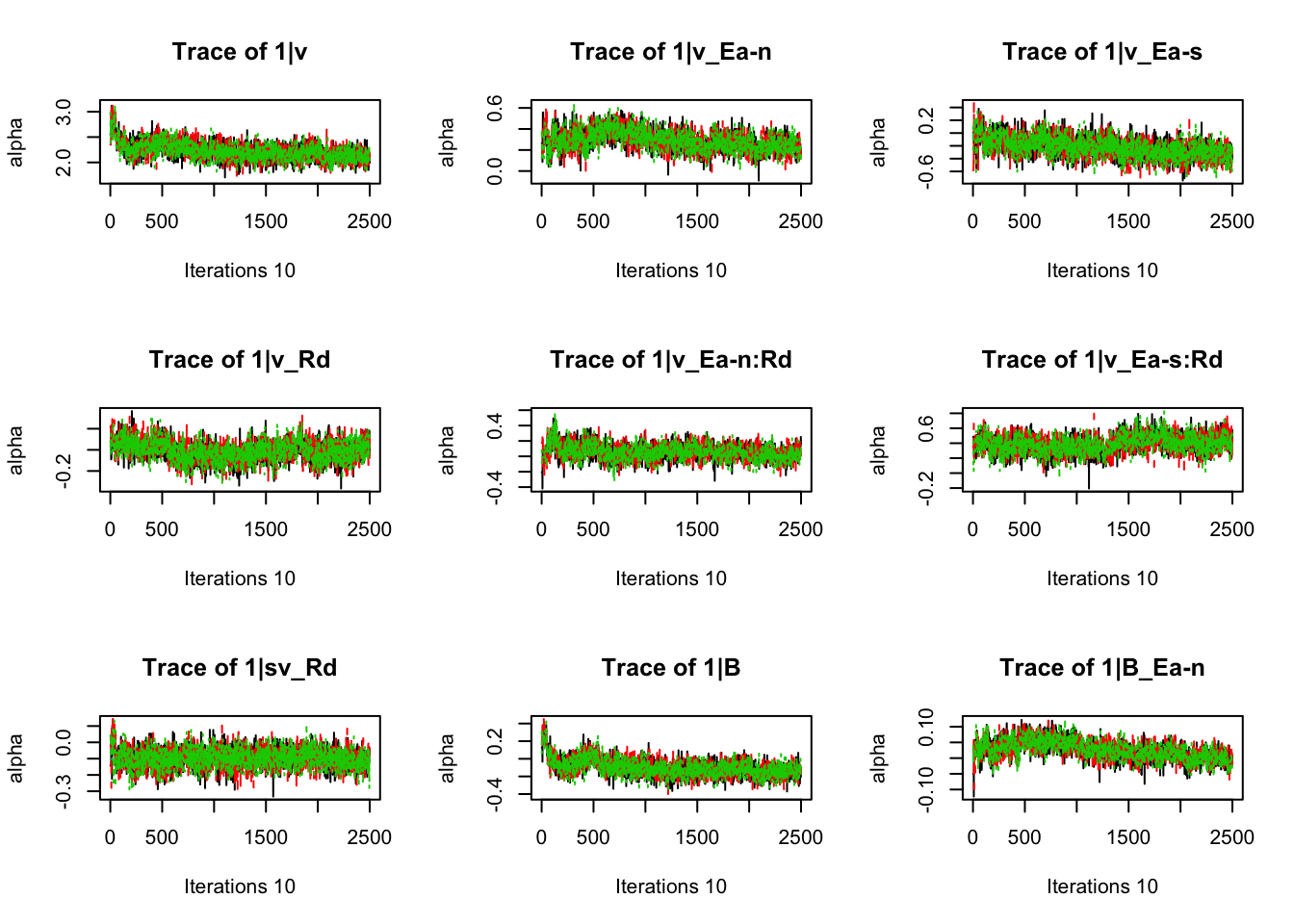
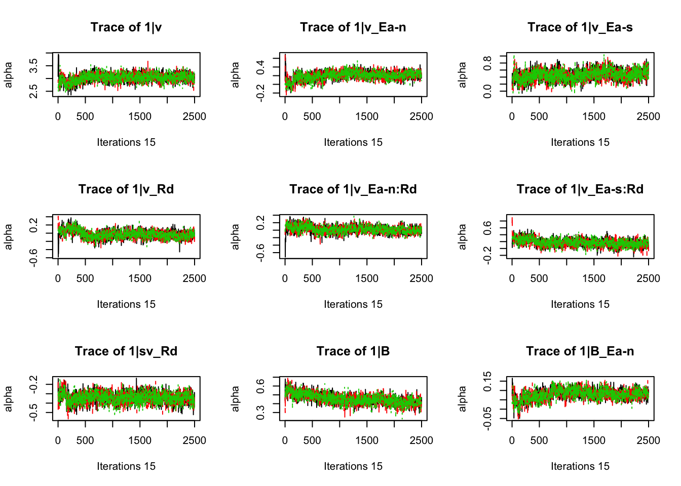
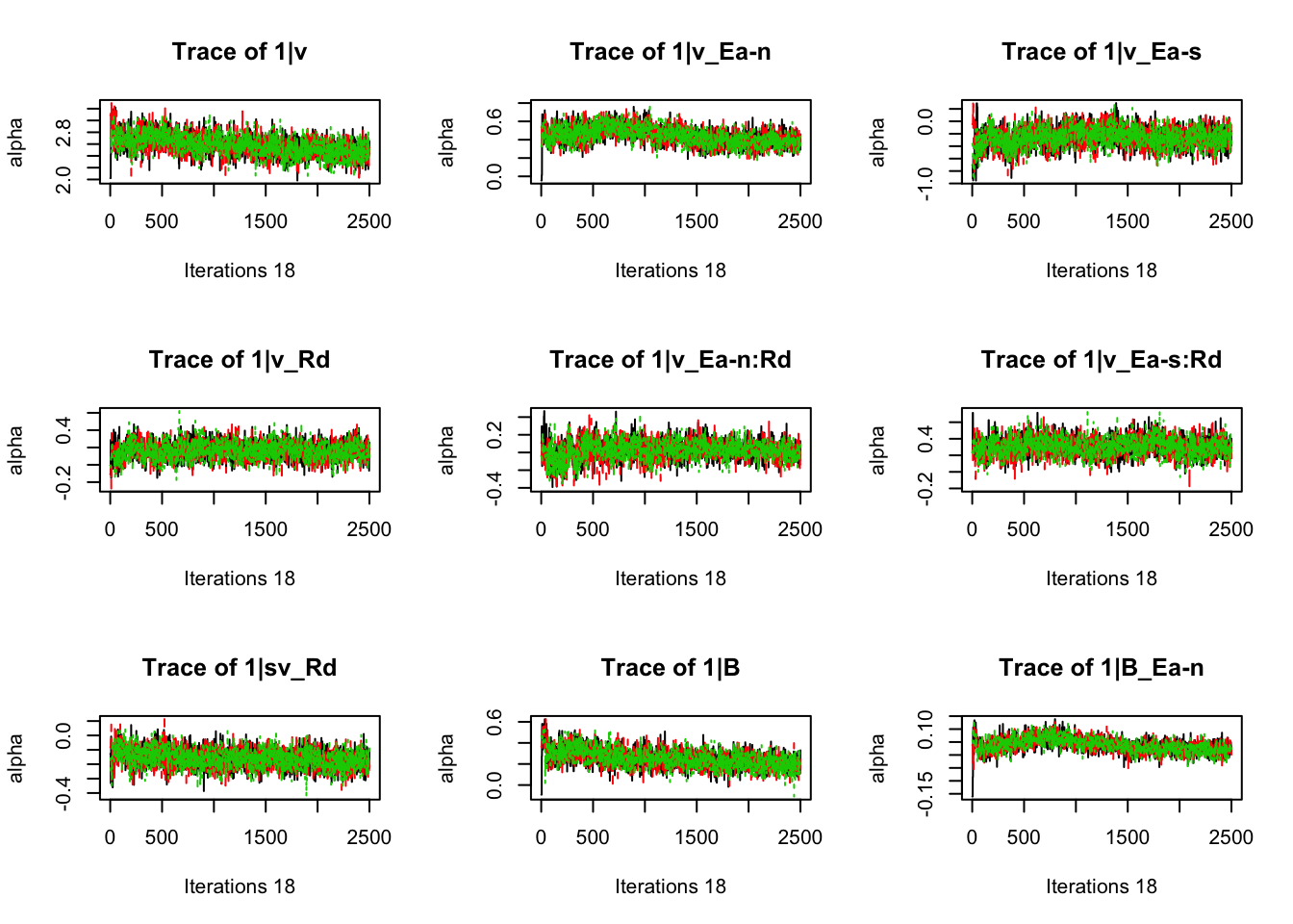
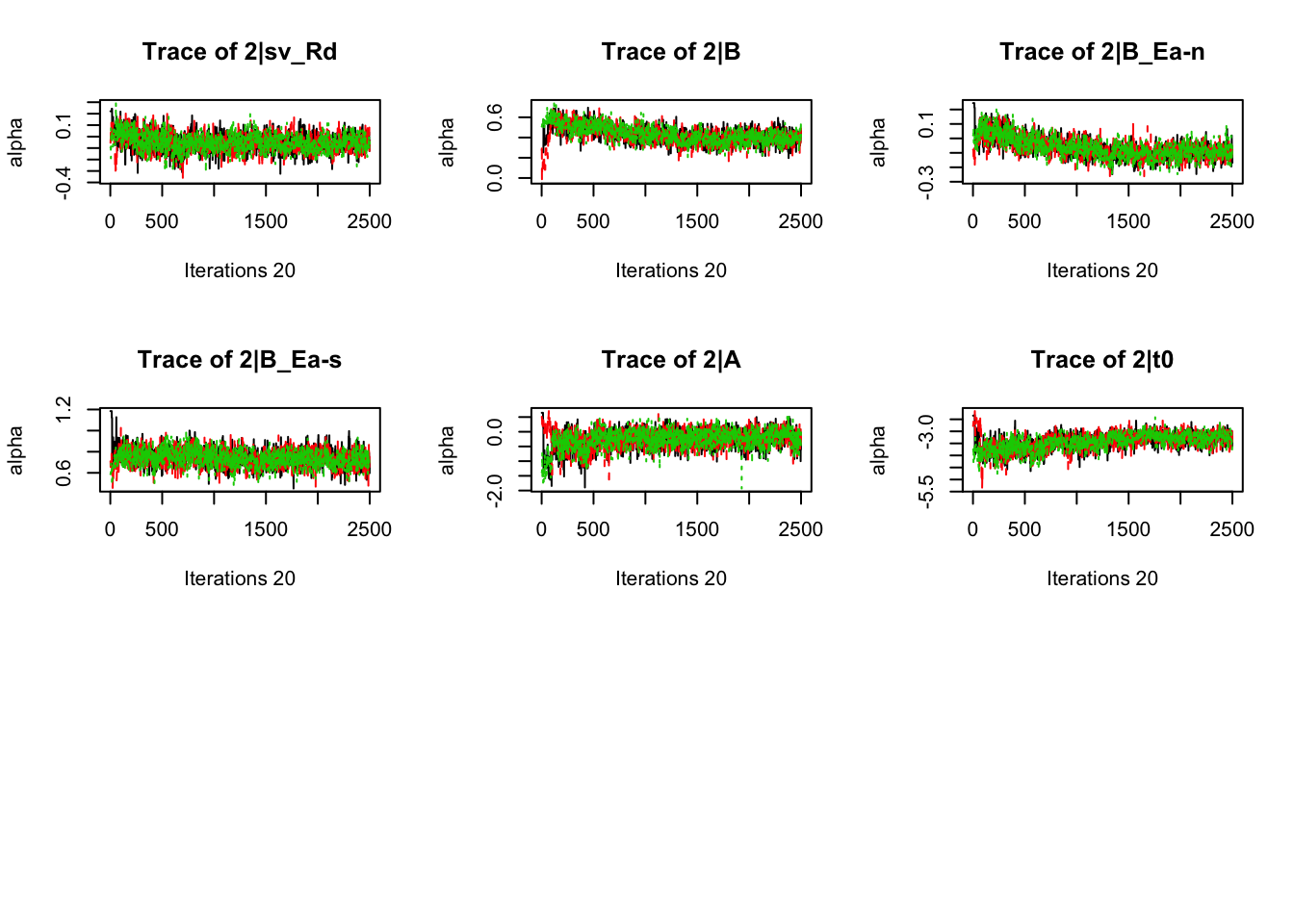
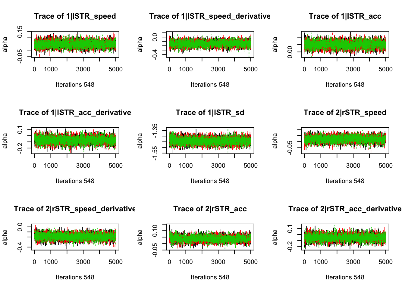
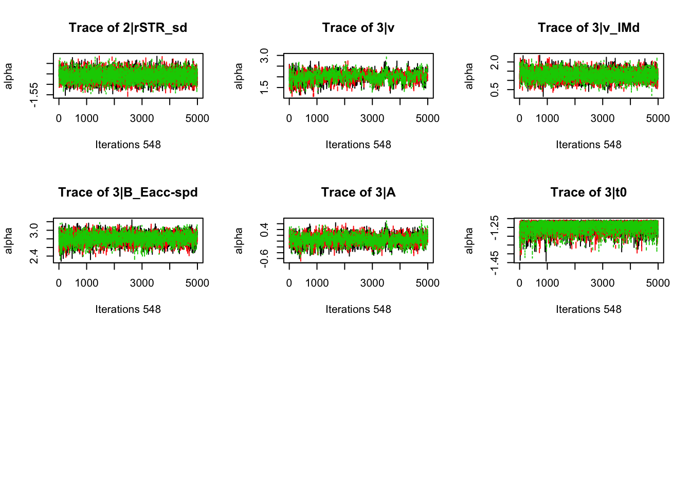
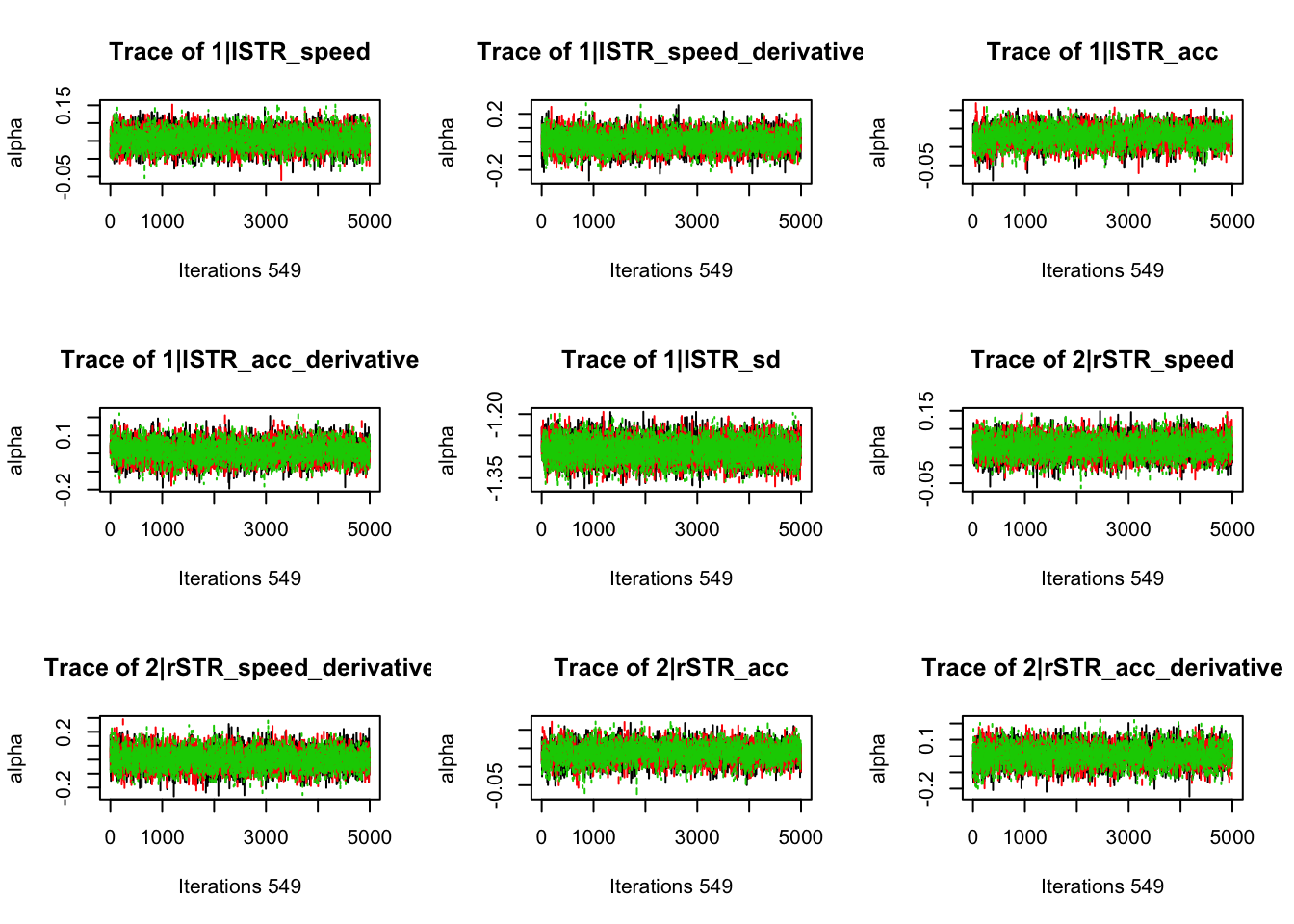
load("~/Desktop/emc_advanced/vignettes/JointModels/samples/joint_VM2011.RData")plot_chains(samples)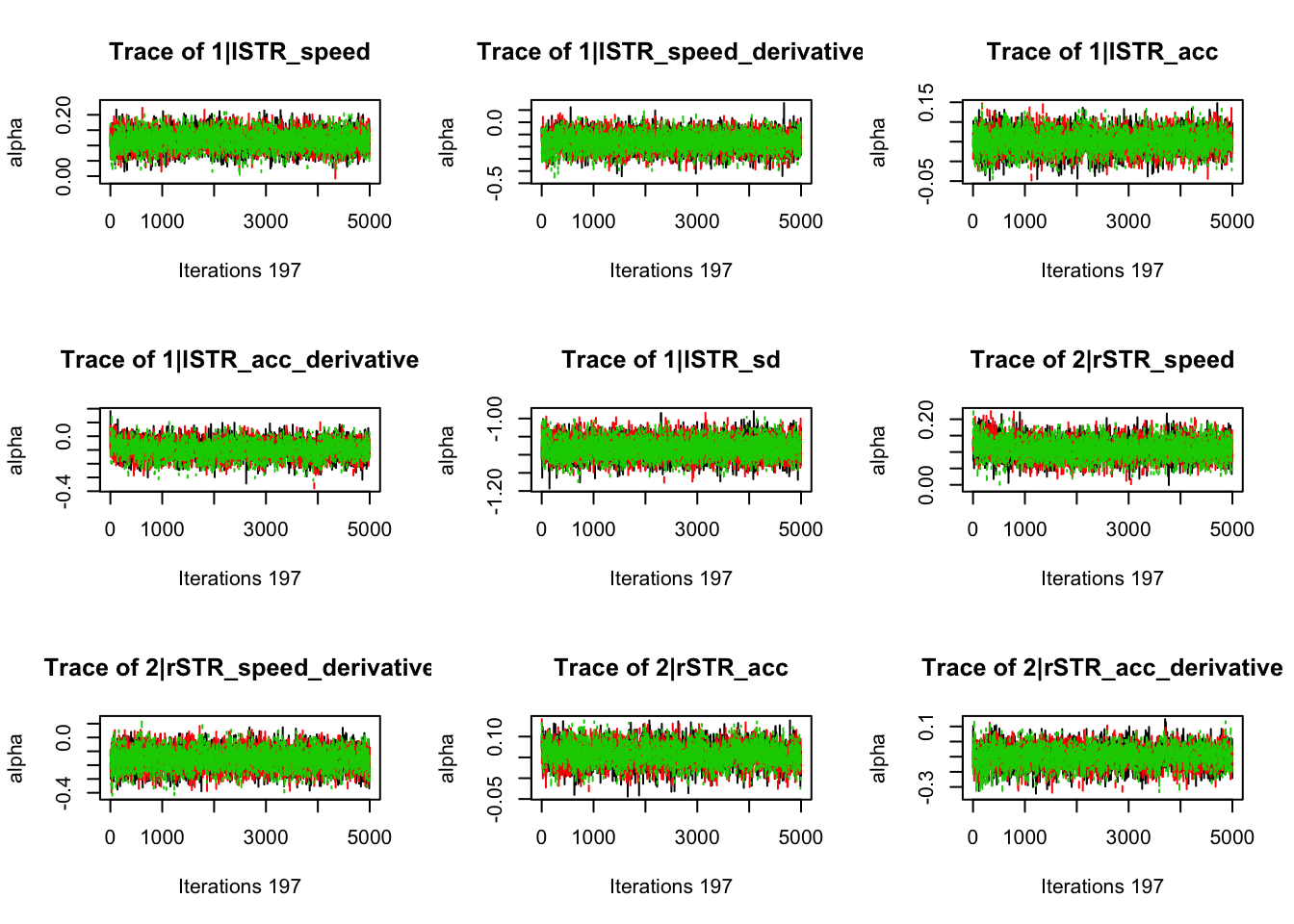
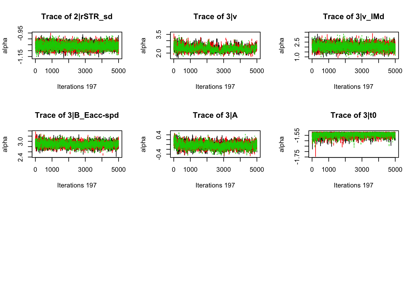
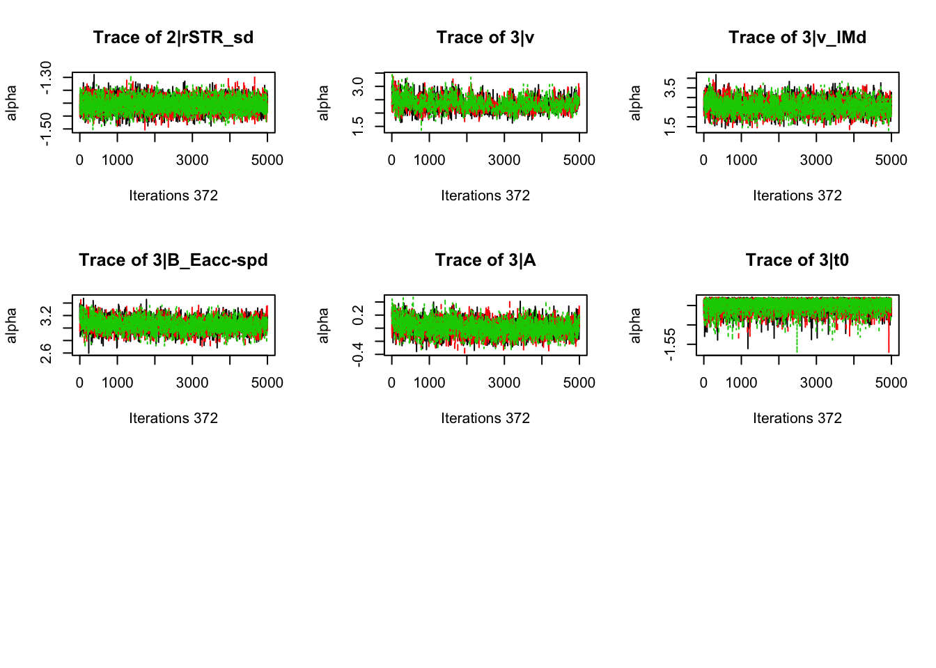
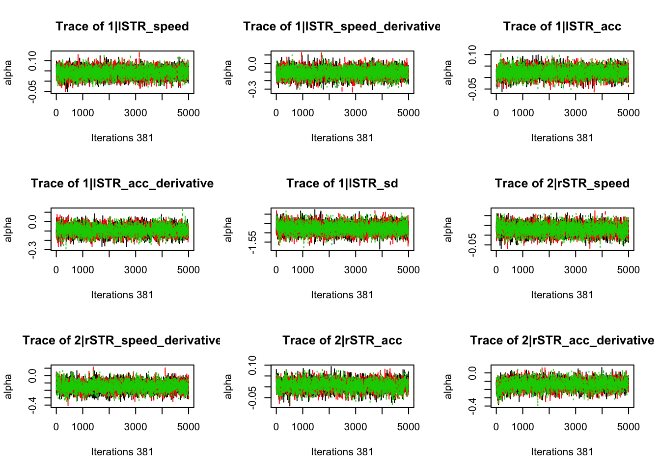
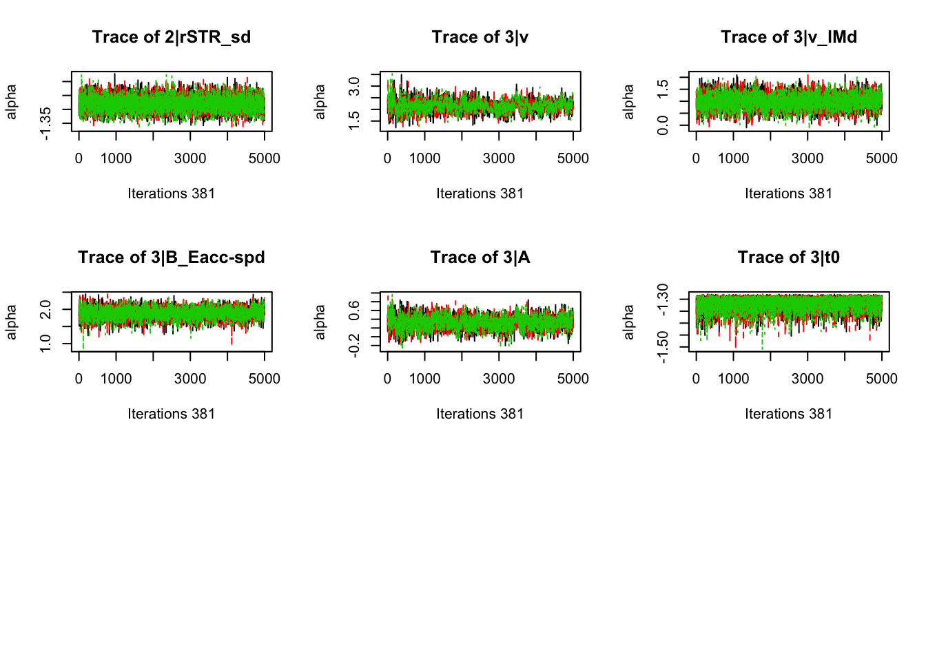
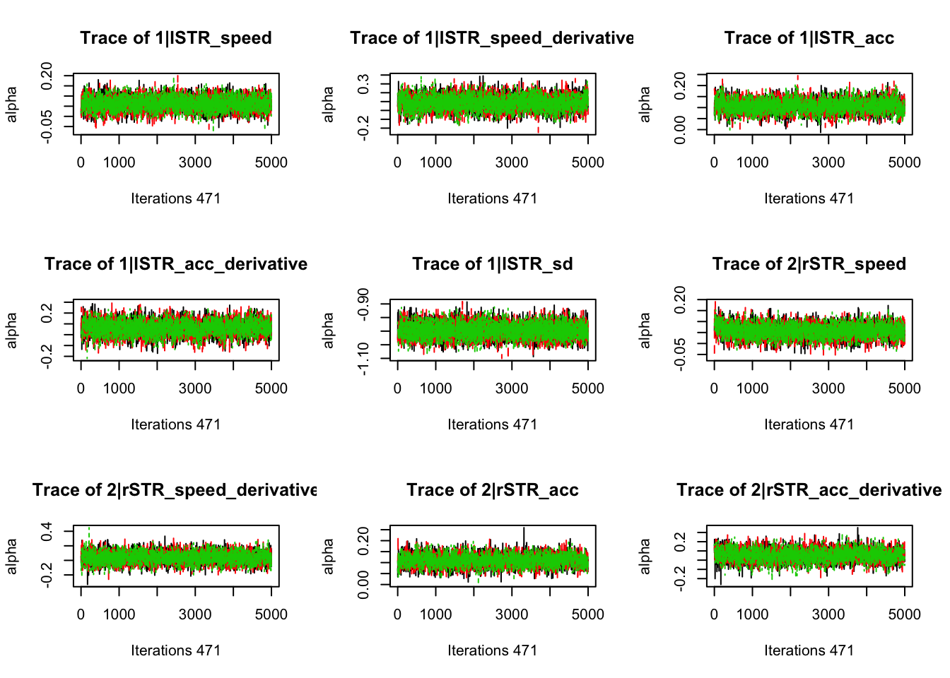
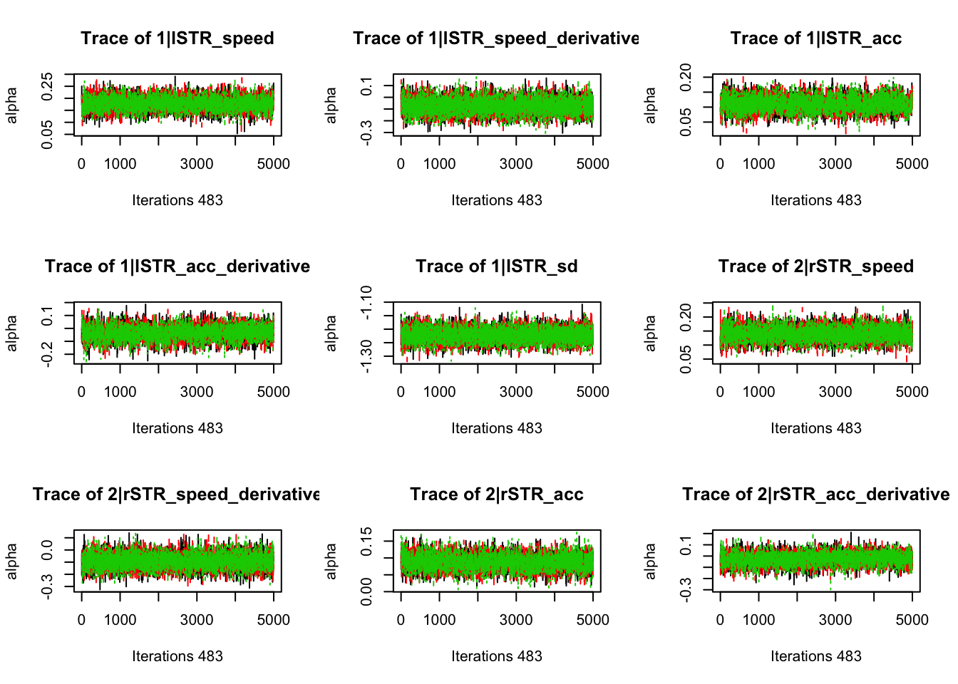
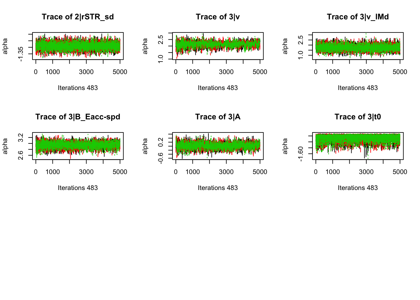
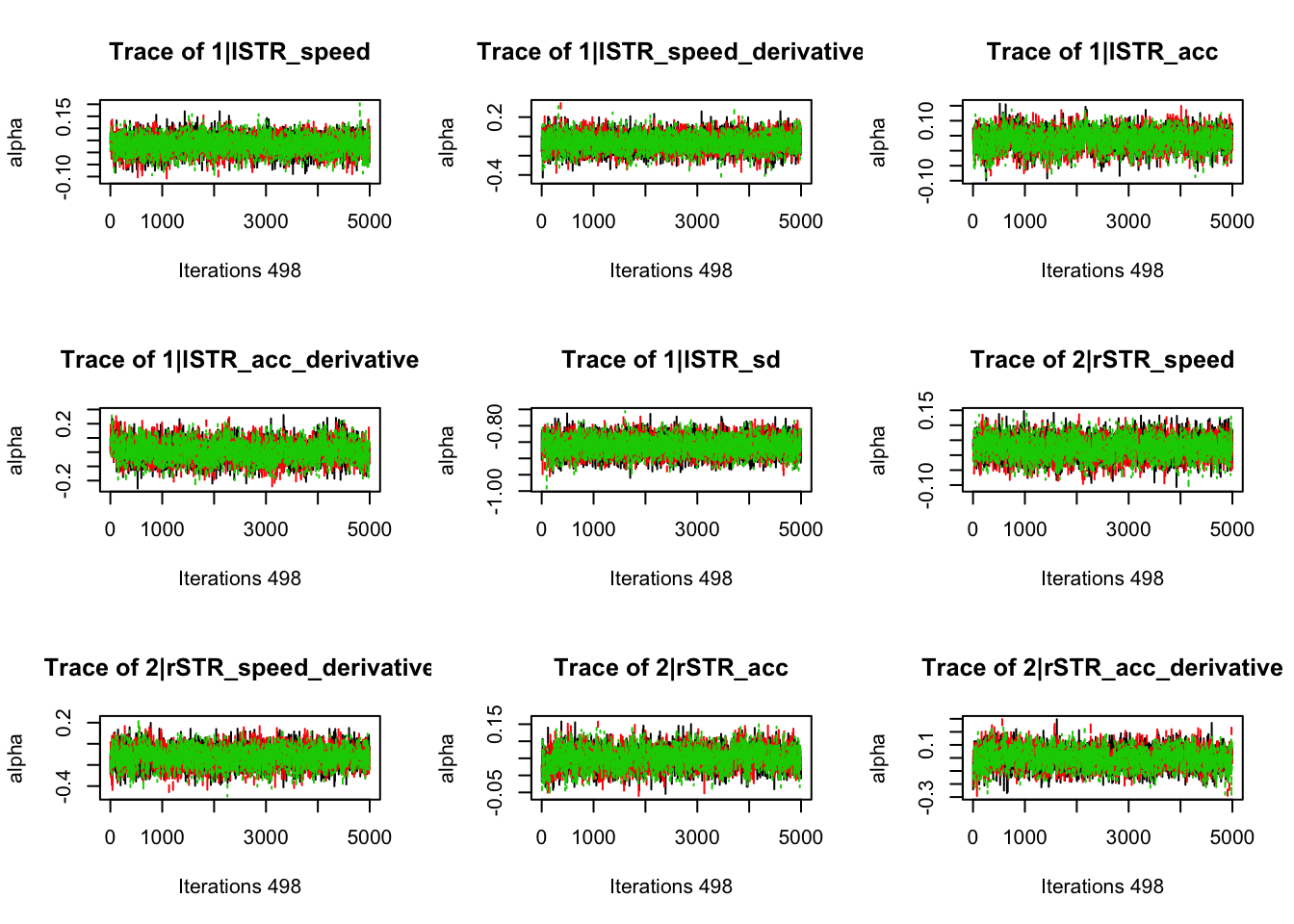
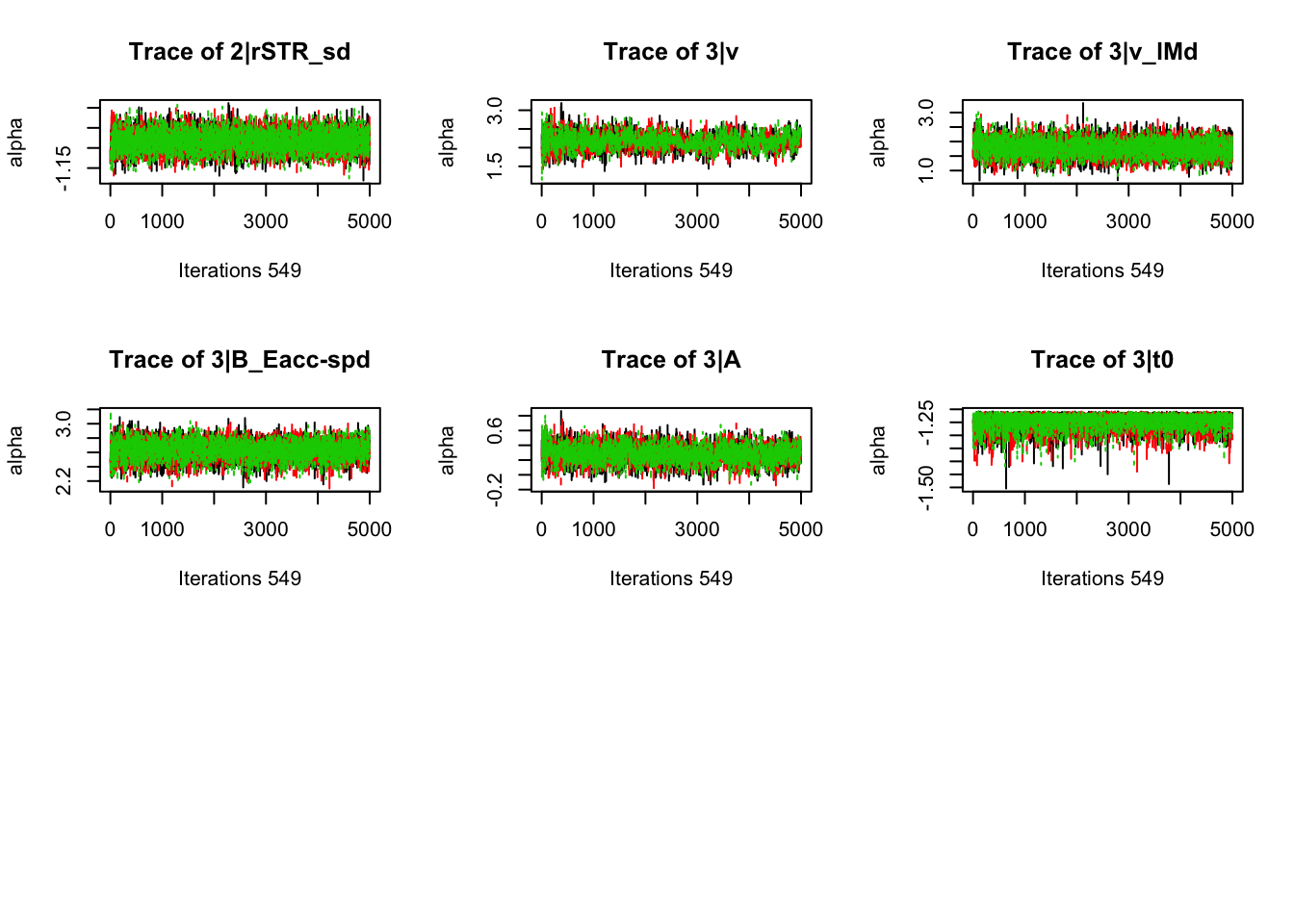
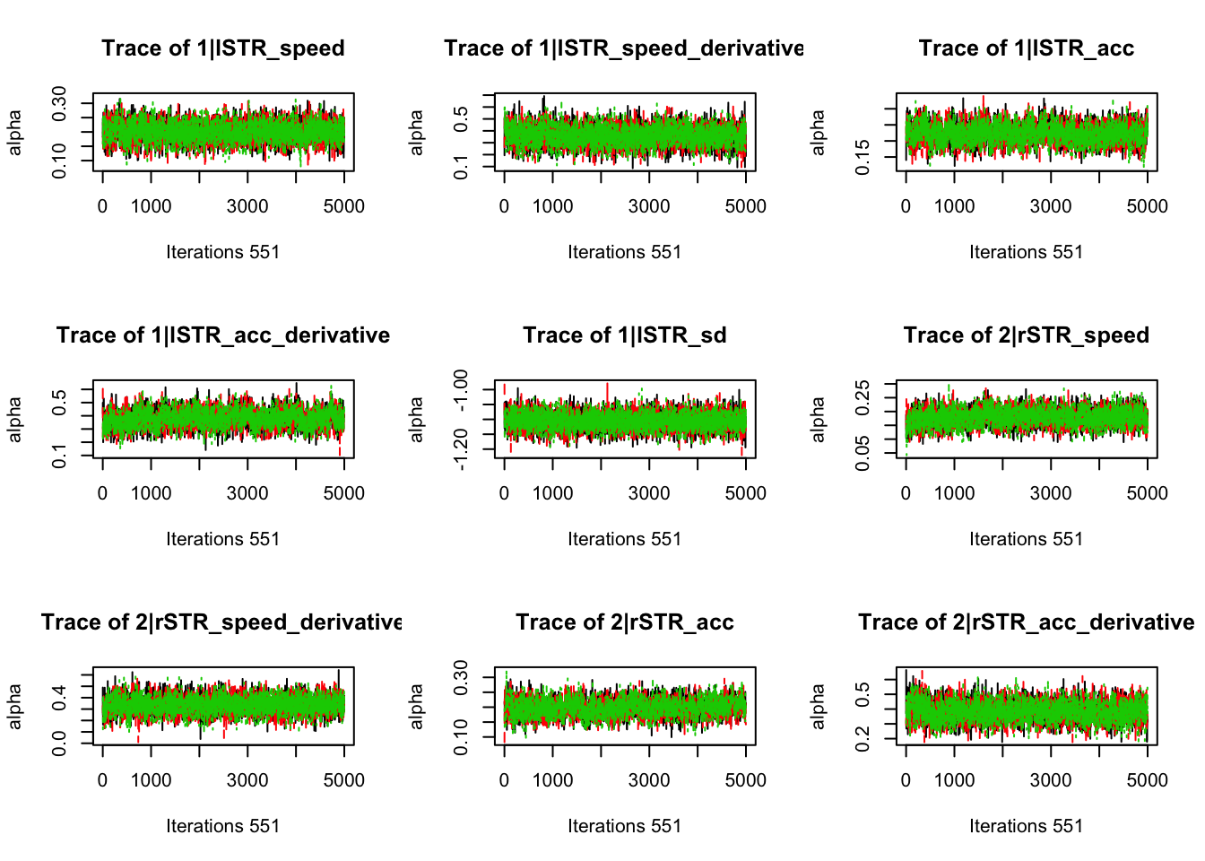
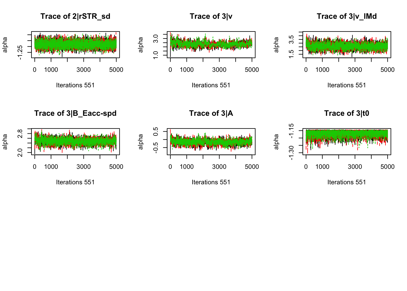
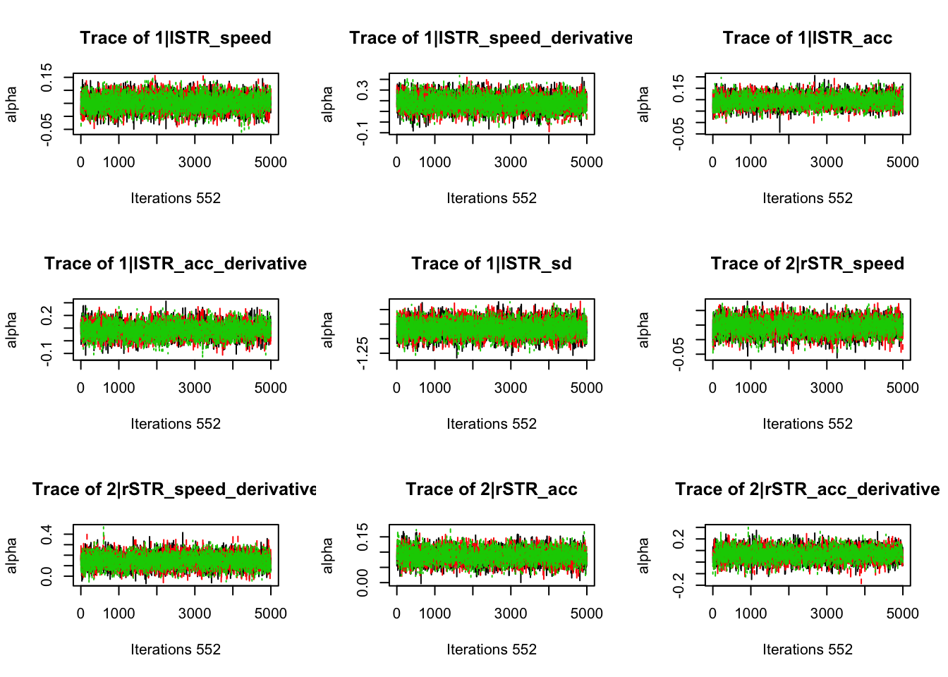

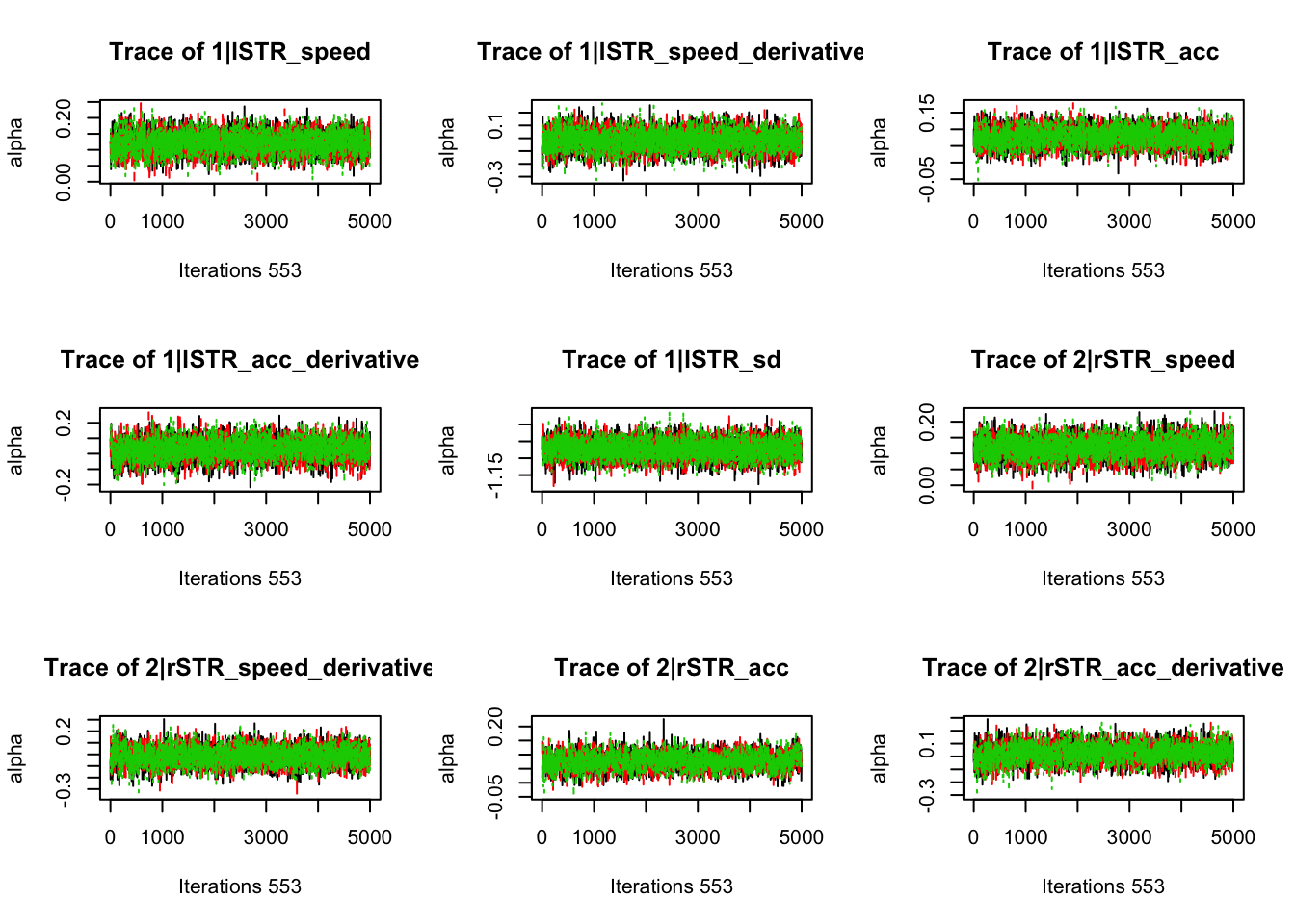
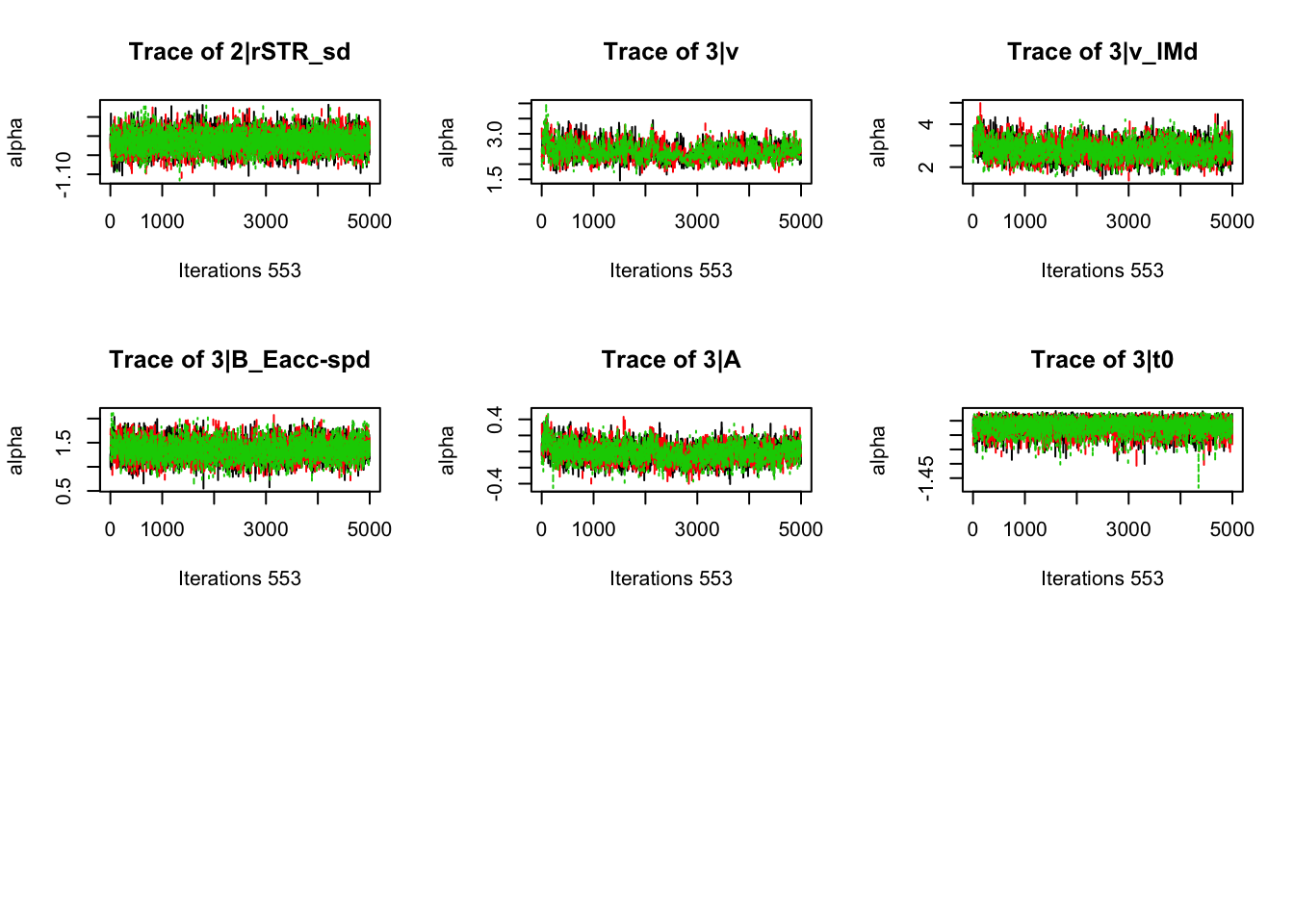
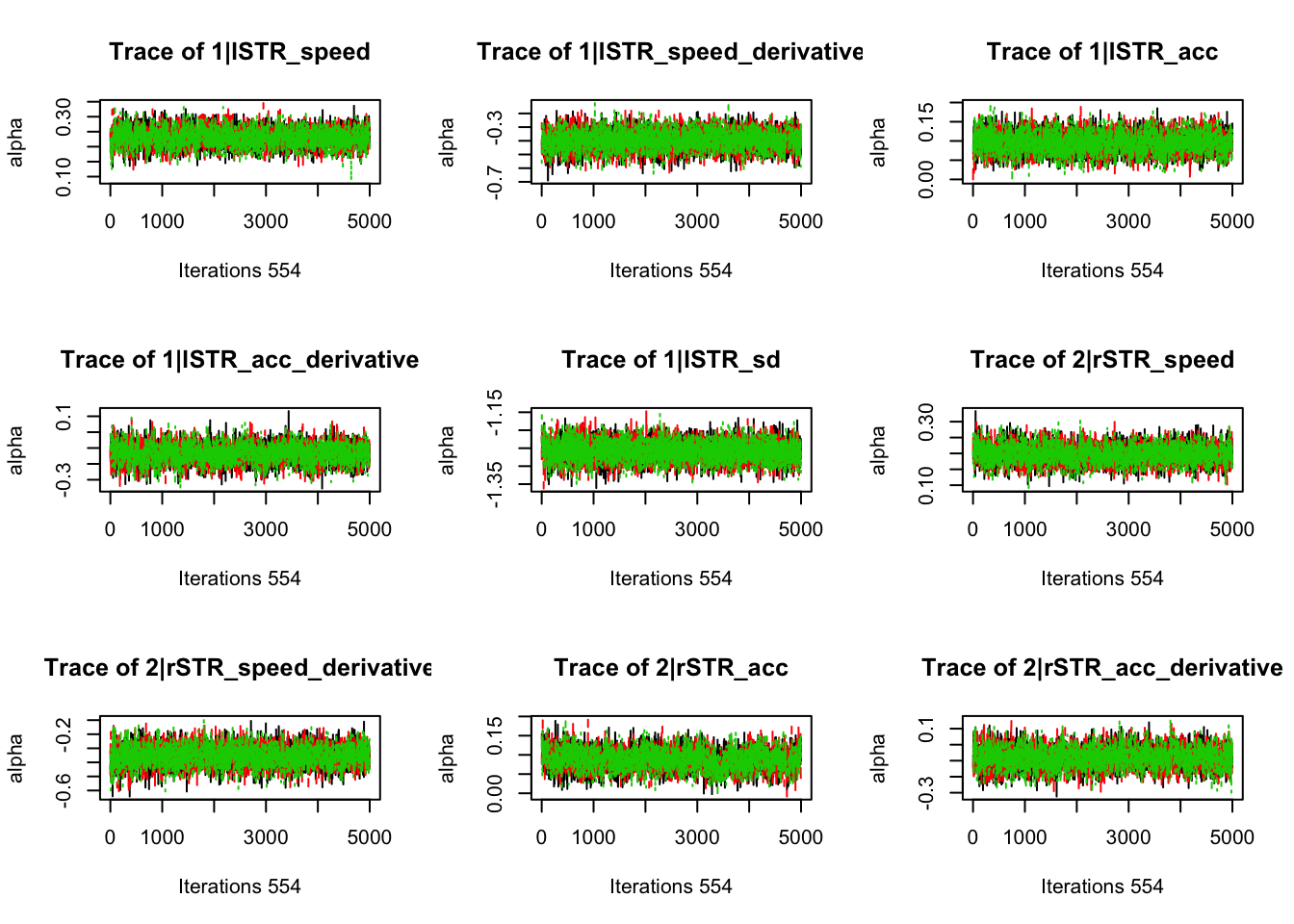
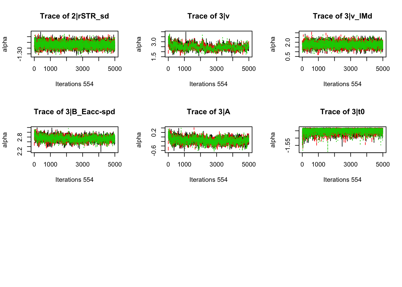
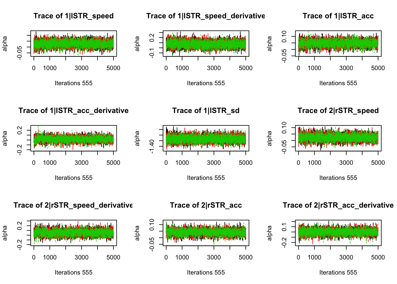
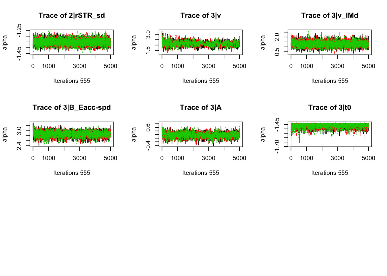
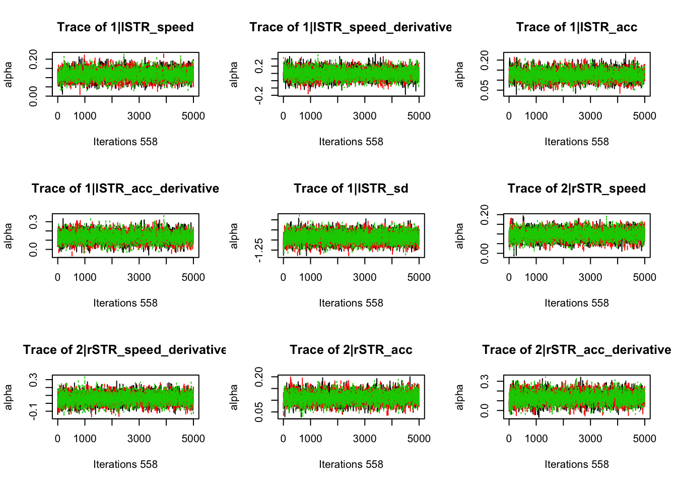
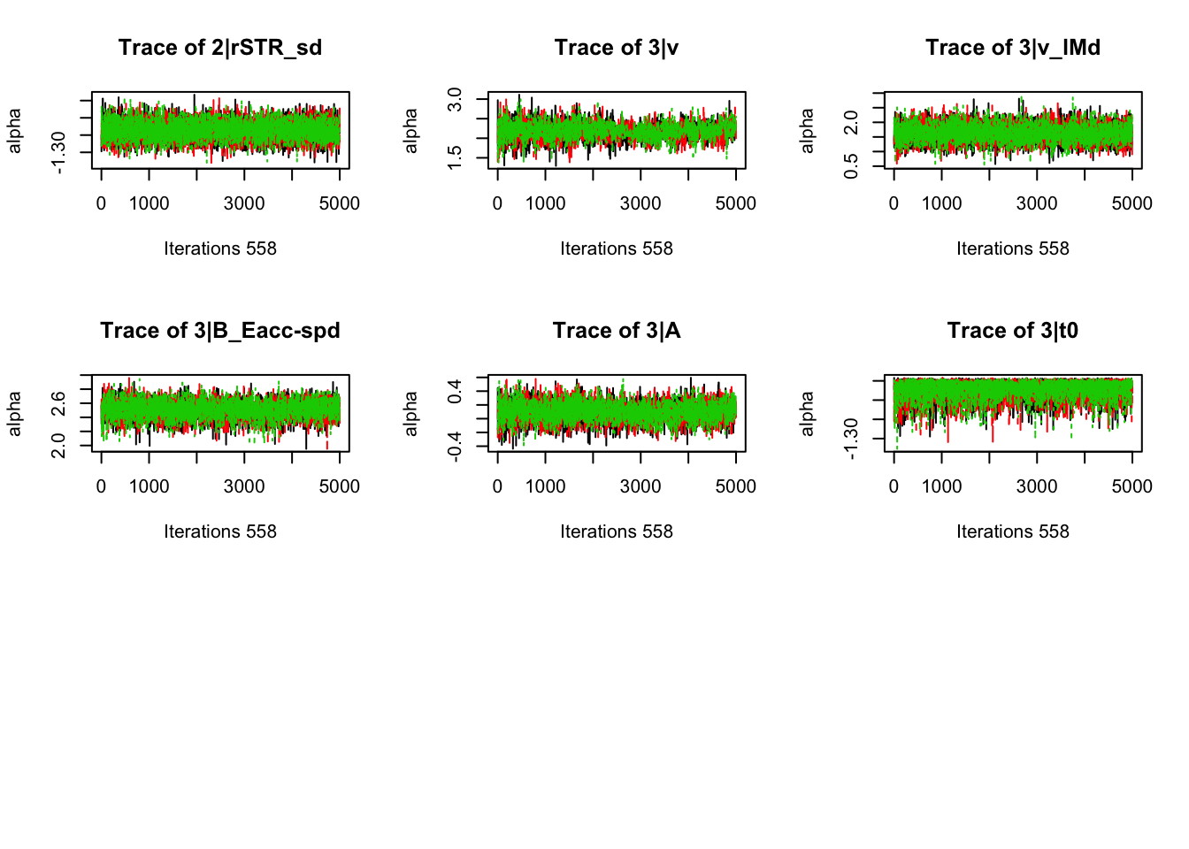
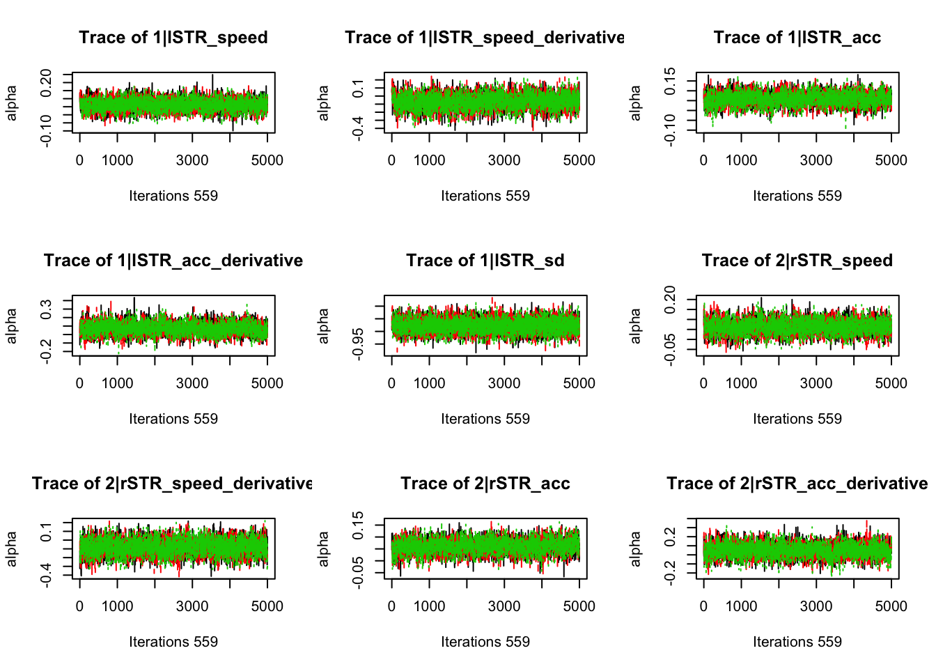
gd_pmwg(samples)## 554 559 523 197 381 544 372 551 553 549 471 498 555 558 548 483 552
## 1.00 1.00 1.00 1.00 1.00 1.00 1.00 1.00 1.00 1.00 1.00 1.00 1.00 1.00 1.01 1.01 1.018.3.3.3 Check fit of the behavioral model
We also want to check how well the model accounts for the behavioral data. For that we need a few different functions. First we split the samples into the part that belonged the behavioral model (the third model we added). Then we run the plot_fit on those samples separately.
samples_behav <- single_out_joint(samples, 3)
pp_behav <- post_predict(samples_behav,n_cores=1, filter = "sample", subfilter = 500)
plot_fit(behav_data,pp_behav,layout=c(2,2),factors=c("E","S"),lpos="right",xlim=c(.25,1.5))     # aggregate over subjects and plot 'overall' CDFs
So the model isn’t great, and we might test it on different models in the future, but since this is mostly a proof of concept. Let’s analyze the correlations.
8.3.3.4 Analyse Correlations
Here, rather than just looking at the numbers, let’s put this in a graphical format for readability. The corrplot package has some excellent functions for plotting correlations which we will rely on below. Merge_samples, makes sure that all the samples from the different chains are nicely bound together as one chain, so that we can easily make inference on them. The samples are of covariances, so after taking the median, we’ll also want to translate them back to correlations.
samples_merged <- merge_samples(samples)
library(corrplot)
median_corrs <- cov2cor(apply(samples_merged$samples$theta_var, 1:2, median))
corrplot(median_corrs)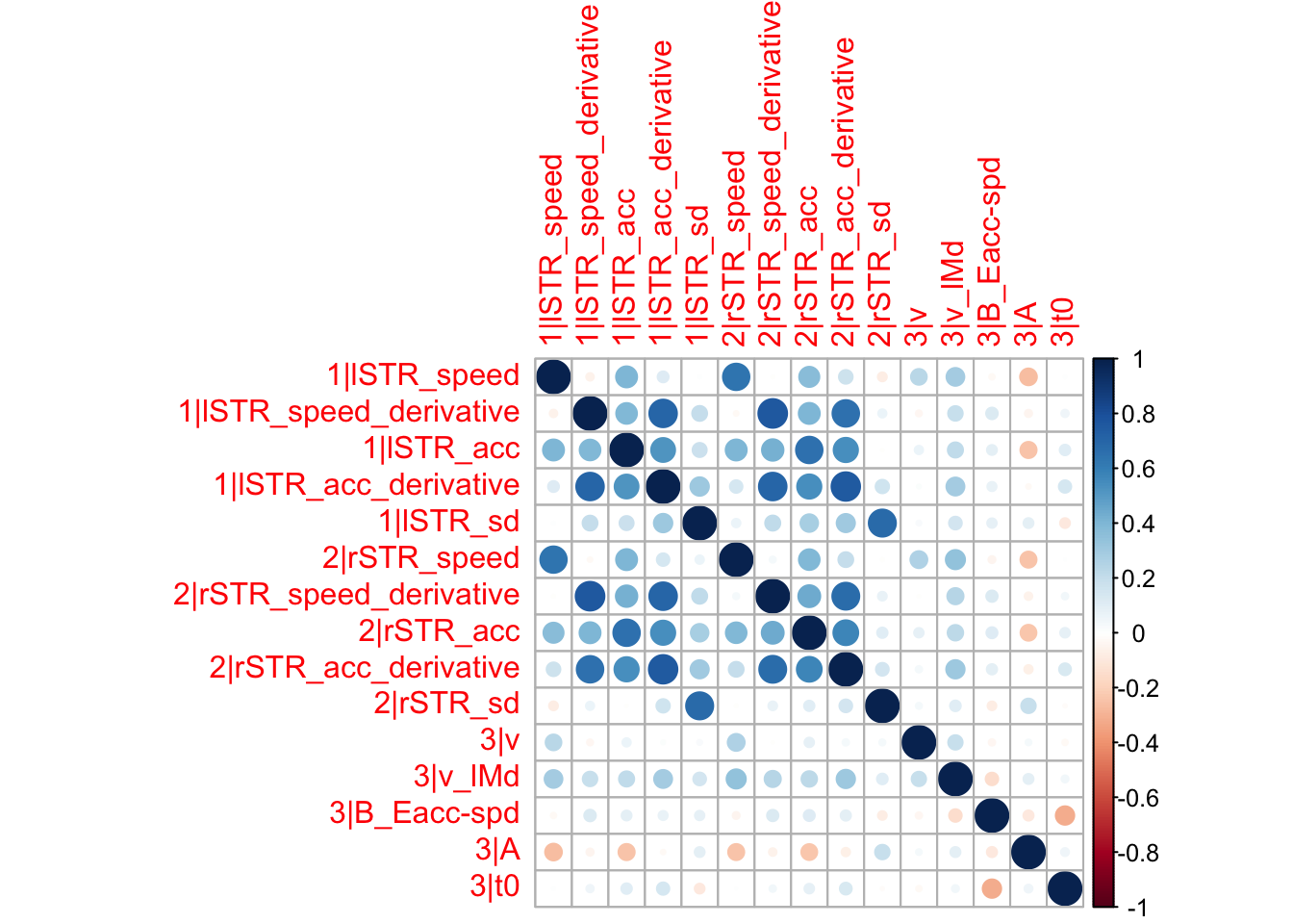
Here we mostly find general correlations between the correct drift rate and the neural activity. More interestingly, the general ‘v’, somewhat like an urgency component, is correlated with both left and right striatal activity during speed cues.
We can also check the distributions of these correlations, since these are part of the sampling process. This highlights the strength of this method; not only are we able to assess correlations between components without attenuation, but we are also able to estimate the level of certainty in these to make stronger, more informed inference.
CIs <- plot_density(samples,layout=c(2,4),selection="correlation", filter = "sample", do_plot=T)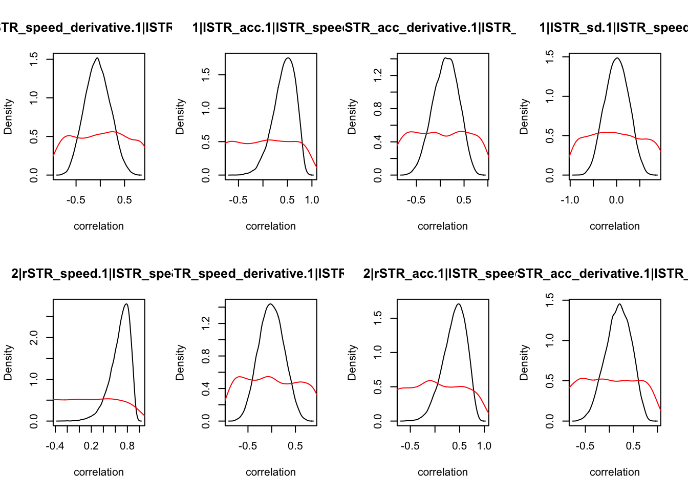
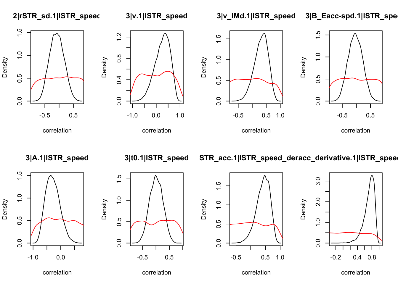
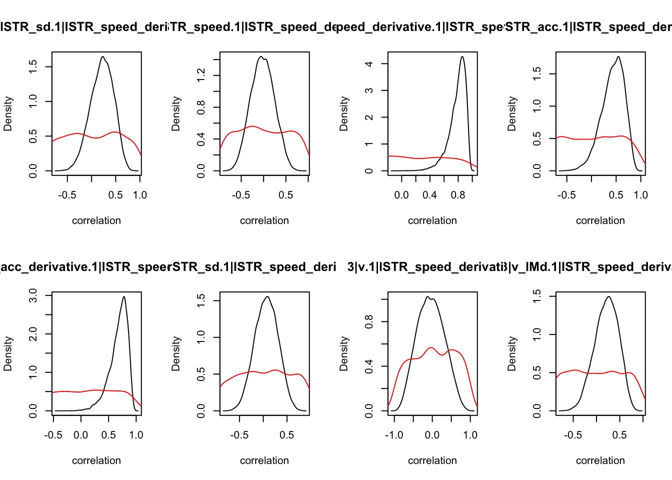
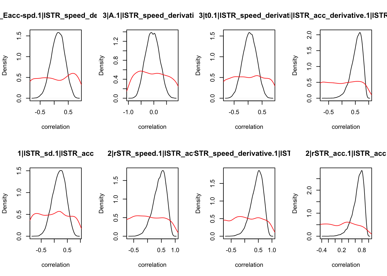
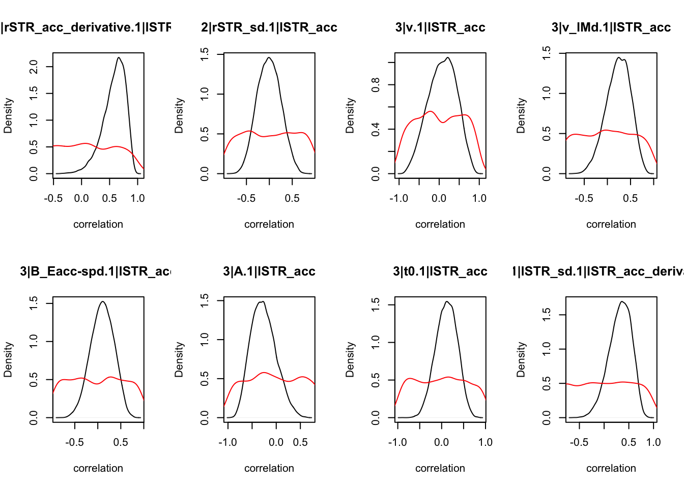
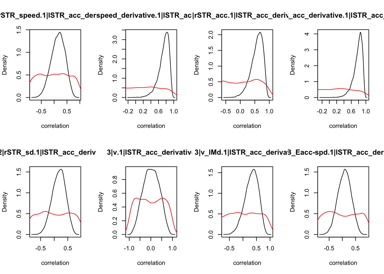
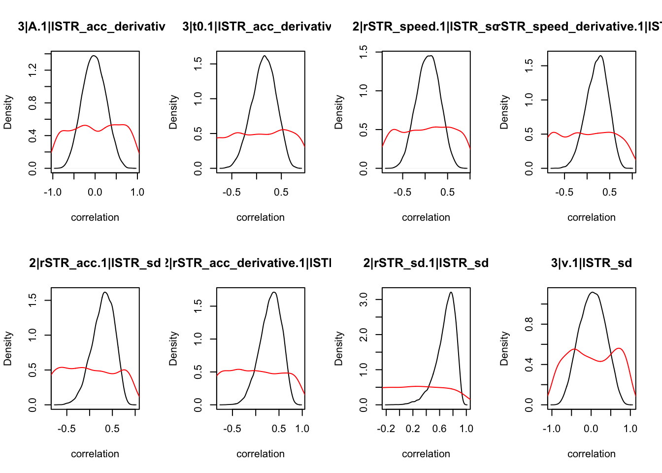
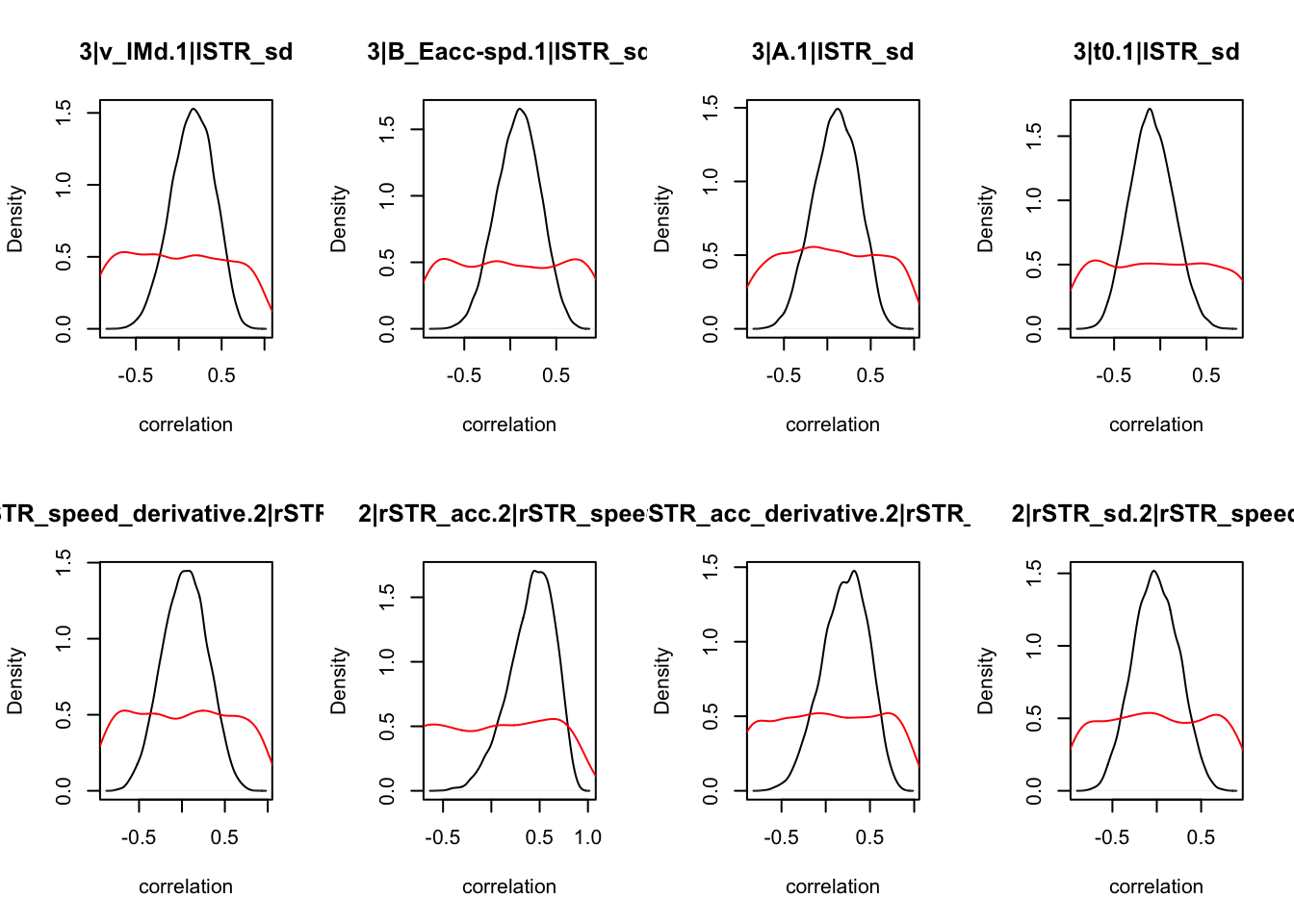
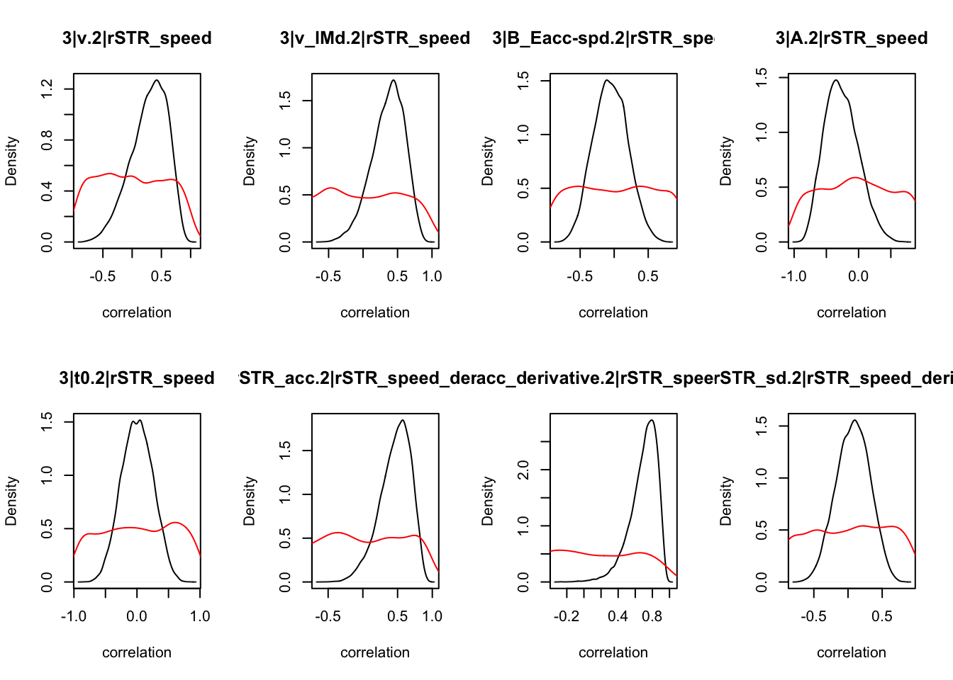
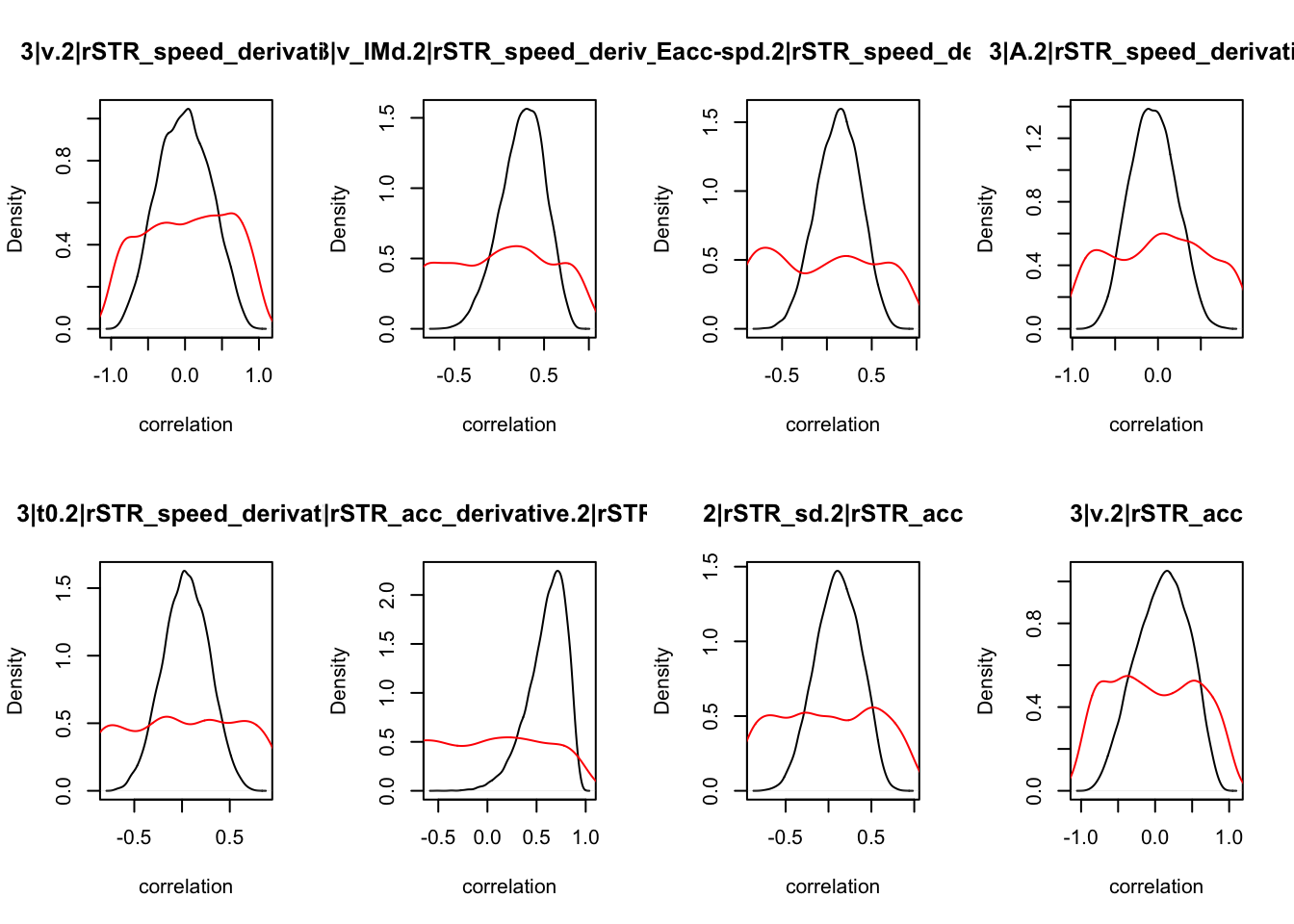
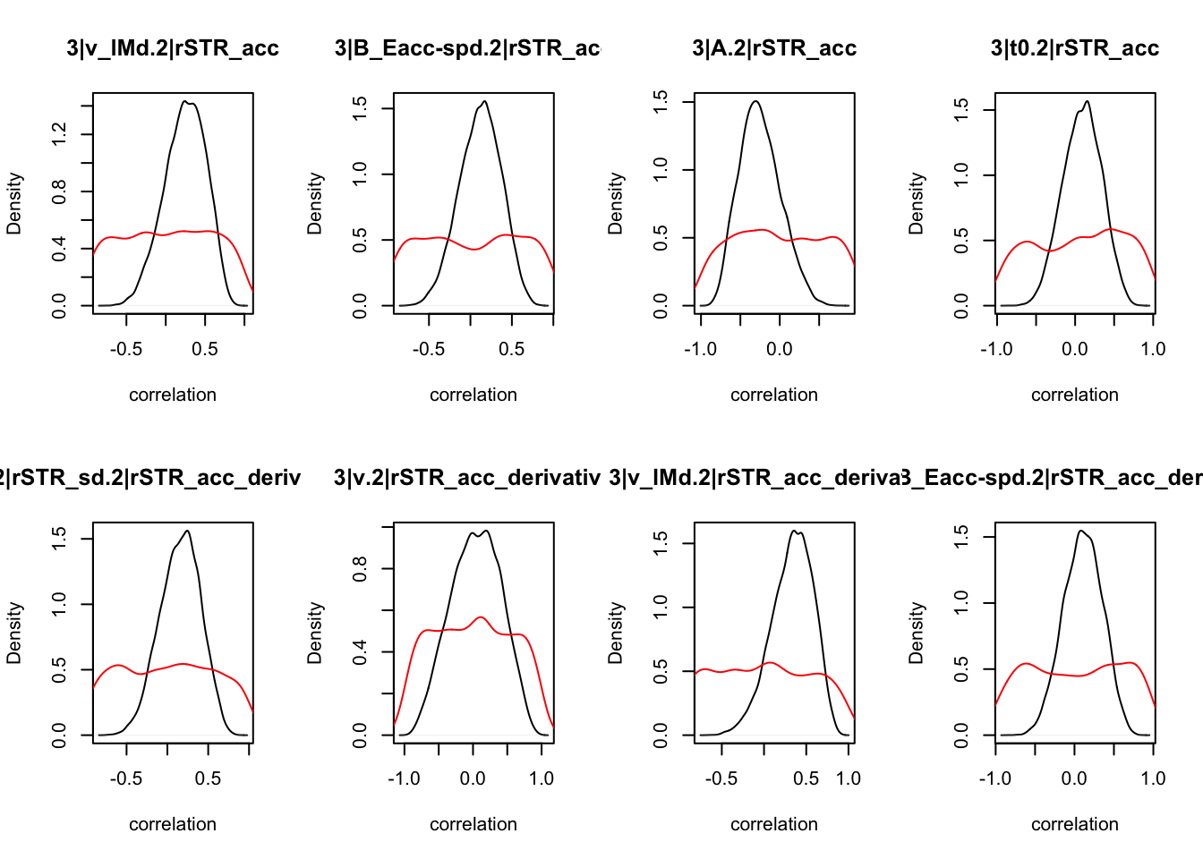
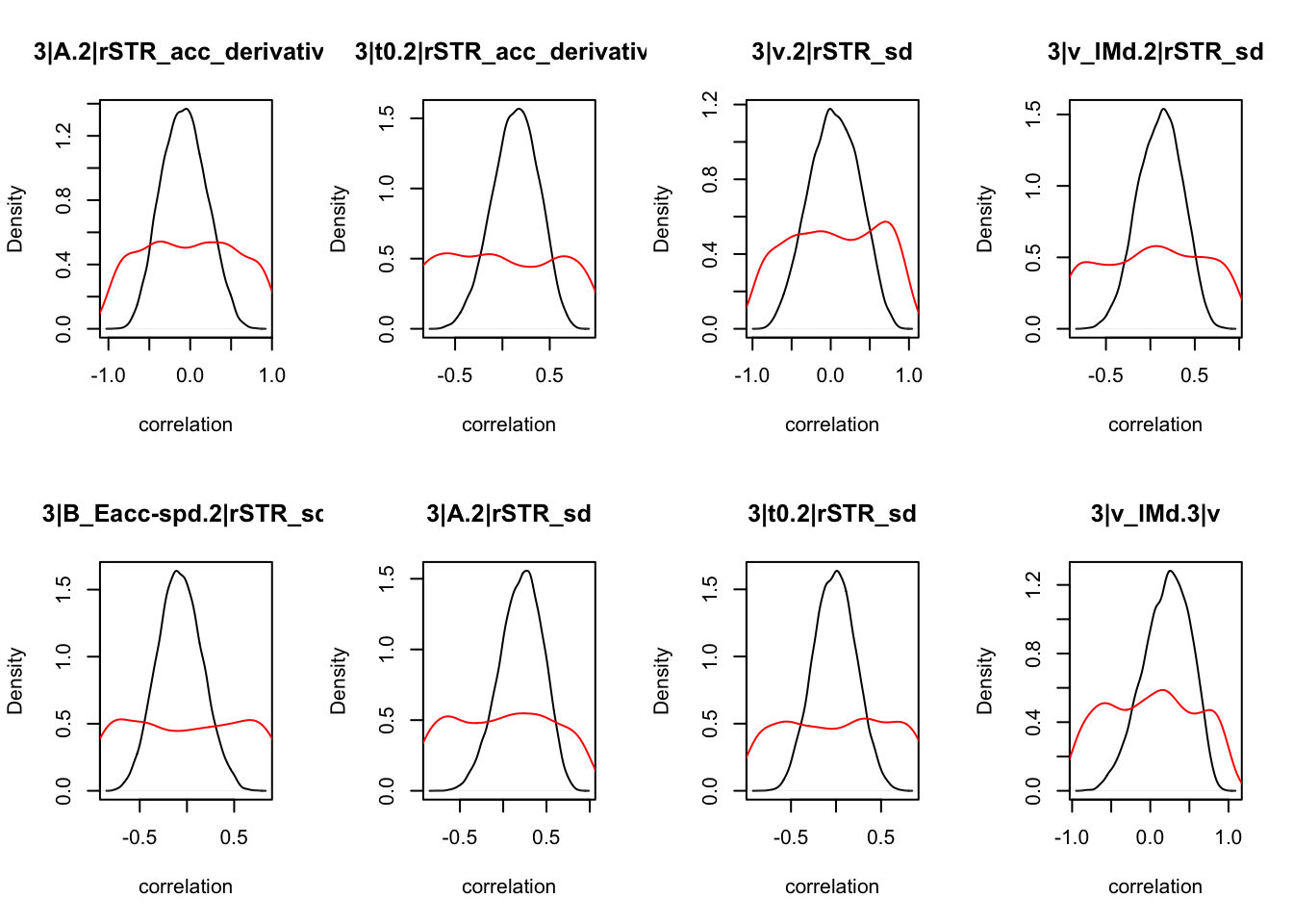
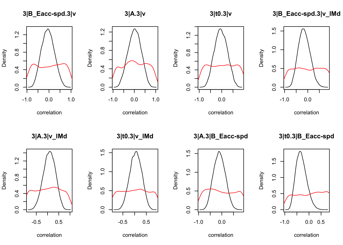
CIs## 1|lSTR_speed_derivative.1|lSTR_speed 1|lSTR_acc.1|lSTR_speed
## 2.5% -0.54259941 -0.05999772
## 50% -0.06084234 0.45888056
## 97.5% 0.44722811 0.79040755
## 1|lSTR_acc_derivative.1|lSTR_speed 1|lSTR_sd.1|lSTR_speed
## 2.5% -0.4113570 -0.472728381
## 50% 0.1247150 0.006734525
## 97.5% 0.5940867 0.479556975
## 2|rSTR_speed.1|lSTR_speed 2|rSTR_speed_derivative.1|lSTR_speed
## 2.5% 0.2724470 -0.503638851
## 50% 0.7076398 -0.009435023
## 97.5% 0.9041650 0.489783107
## 2|rSTR_acc.1|lSTR_speed 2|rSTR_acc_derivative.1|lSTR_speed
## 2.5% -0.1096638 -0.3461710
## 50% 0.4235517 0.1972929
## 97.5% 0.7762978 0.6516647
## 2|rSTR_sd.1|lSTR_speed 3|v.1|lSTR_speed 3|v_lMd.1|lSTR_speed
## 2.5% -0.54105741 -0.4023101 -0.2026096
## 50% -0.08295503 0.2927532 0.3388171
## 97.5% 0.40663463 0.7653636 0.7241655
## 3|B_Eacc-spd.1|lSTR_speed 3|A.1|lSTR_speed 3|t0.1|lSTR_speed
## 2.5% -0.5084157 -0.7180179 -0.457042885
## 50% -0.0366106 -0.3037498 0.009624853
## 97.5% 0.4432043 0.2409130 0.475765614
## 1|lSTR_acc.1|lSTR_speed_derivative
## 2.5% -0.08578338
## 50% 0.44134047
## 97.5% 0.78502490
## 1|lSTR_acc_derivative.1|lSTR_speed_derivative
## 2.5% 0.3739149
## 50% 0.7542055
## 97.5% 0.9230135
## 1|lSTR_sd.1|lSTR_speed_derivative 2|rSTR_speed.1|lSTR_speed_derivative
## 2.5% -0.2656937 -0.51628978
## 50% 0.2269470 -0.02475963
## 97.5% 0.6278837 0.47873860
## 2|rSTR_speed_derivative.1|lSTR_speed_derivative
## 2.5% 0.4856749
## 50% 0.8164267
## 97.5% 0.9439046
## 2|rSTR_acc.1|lSTR_speed_derivative
## 2.5% -0.0707833
## 50% 0.4566680
## 97.5% 0.7977546
## 2|rSTR_acc_derivative.1|lSTR_speed_derivative
## 2.5% 0.2795418
## 50% 0.7133267
## 97.5% 0.9056038
## 2|rSTR_sd.1|lSTR_speed_derivative 3|v.1|lSTR_speed_derivative
## 2.5% -0.40910294 -0.68293345
## 50% 0.06879554 -0.04616012
## 97.5% 0.52393744 0.63609485
## 3|v_lMd.1|lSTR_speed_derivative 3|B_Eacc-spd.1|lSTR_speed_derivative
## 2.5% -0.3020323 -0.3438495
## 50% 0.2272557 0.1378982
## 97.5% 0.6563621 0.5799020
## 3|A.1|lSTR_speed_derivative 3|t0.1|lSTR_speed_derivative
## 2.5% -0.55103865 -0.41206860
## 50% -0.05578916 0.05697376
## 97.5% 0.45769307 0.51010188
## 1|lSTR_acc_derivative.1|lSTR_acc 1|lSTR_sd.1|lSTR_acc 2|rSTR_speed.1|lSTR_acc
## 2.5% 0.0693568 -0.3119654 -0.08525178
## 50% 0.5824347 0.2025122 0.46378548
## 97.5% 0.8574358 0.6403175 0.79968650
## 2|rSTR_speed_derivative.1|lSTR_acc 2|rSTR_acc.1|lSTR_acc
## 2.5% -0.05067311 0.2873053
## 50% 0.47663913 0.7172036
## 97.5% 0.80467033 0.9135155
## 2|rSTR_acc_derivative.1|lSTR_acc 2|rSTR_sd.1|lSTR_acc 3|v.1|lSTR_acc
## 2.5% 0.1121583 -0.488170518 -0.60565935
## 50% 0.6122200 -0.008821304 0.09572427
## 97.5% 0.8768836 0.488265961 0.70446813
## 3|v_lMd.1|lSTR_acc 3|B_Eacc-spd.1|lSTR_acc 3|A.1|lSTR_acc 3|t0.1|lSTR_acc
## 2.5% -0.3063548 -0.4031381 -0.7033076 -0.3734026
## 50% 0.2483585 0.1023404 -0.2785996 0.1159725
## 97.5% 0.6901886 0.5565351 0.2776972 0.5532912
## 1|lSTR_sd.1|lSTR_acc_derivative 2|rSTR_speed.1|lSTR_acc_derivative
## 2.5% -0.1651170 -0.3917563
## 50% 0.3415904 0.1667999
## 97.5% 0.7007815 0.6280221
## 2|rSTR_speed_derivative.1|lSTR_acc_derivative 2|rSTR_acc.1|lSTR_acc_derivative
## 2.5% 0.3806950 0.08786324
## 50% 0.7648677 0.60279296
## 97.5% 0.9266506 0.87148231
## 2|rSTR_acc_derivative.1|lSTR_acc_derivative 2|rSTR_sd.1|lSTR_acc_derivative
## 2.5% 0.4638641 -0.3238653
## 50% 0.8070927 0.1817609
## 97.5% 0.9422813 0.6113298
## 3|v.1|lSTR_acc_derivative 3|v_lMd.1|lSTR_acc_derivative
## 2.5% -0.66345421 -0.2040681
## 50% 0.01920316 0.3408452
## 97.5% 0.68199482 0.7327866
## 3|B_Eacc-spd.1|lSTR_acc_derivative 3|A.1|lSTR_acc_derivative
## 2.5% -0.40705452 -0.54201301
## 50% 0.08729069 -0.02531149
## 97.5% 0.54794454 0.49767981
## 3|t0.1|lSTR_acc_derivative 2|rSTR_speed.1|lSTR_sd
## 2.5% -0.3358167 -0.42290714
## 50% 0.1560790 0.07329141
## 97.5% 0.5822285 0.54532575
## 2|rSTR_speed_derivative.1|lSTR_sd 2|rSTR_acc.1|lSTR_sd
## 2.5% -0.2655676 -0.2173979
## 50% 0.2344844 0.3177121
## 97.5% 0.6393508 0.7055699
## 2|rSTR_acc_derivative.1|lSTR_sd 2|rSTR_sd.1|lSTR_sd 3|v.1|lSTR_sd
## 2.5% -0.1652611 0.3279681 -0.57832285
## 50% 0.3409141 0.7187307 0.03719717
## 97.5% 0.7076399 0.8982774 0.62943517
## 3|v_lMd.1|lSTR_sd 3|B_Eacc-spd.1|lSTR_sd 3|A.1|lSTR_sd 3|t0.1|lSTR_sd
## 2.5% -0.3406758 -0.38338678 -0.4048585 -0.5222247
## 50% 0.1678200 0.09217298 0.1063171 -0.0981749
## 97.5% 0.6032046 0.52598190 0.5580193 0.3709208
## 2|rSTR_speed_derivative.2|rSTR_speed 2|rSTR_acc.2|rSTR_speed
## 2.5% -0.47280546 -0.09741634
## 50% 0.03883041 0.44178606
## 97.5% 0.52597512 0.79152501
## 2|rSTR_acc_derivative.2|rSTR_speed 2|rSTR_sd.2|rSTR_speed 3|v.2|rSTR_speed
## 2.5% -0.3181124 -0.49742889 -0.3882852
## 50% 0.2308385 -0.01235487 0.3252774
## 97.5% 0.6653034 0.47695472 0.7813950
## 3|v_lMd.2|rSTR_speed 3|B_Eacc-spd.2|rSTR_speed 3|A.2|rSTR_speed
## 2.5% -0.1562044 -0.52302992 -0.7080620
## 50% 0.3868030 -0.05534575 -0.2809184
## 97.5% 0.7559630 0.43693825 0.2819108
## 3|t0.2|rSTR_speed 2|rSTR_acc.2|rSTR_speed_derivative
## 2.5% -0.472652820 -0.03886133
## 50% 0.004412172 0.49391142
## 97.5% 0.475471522 0.81659090
## 2|rSTR_acc_derivative.2|rSTR_speed_derivative
## 2.5% 0.3118715
## 50% 0.7265164
## 97.5% 0.9155086
## 2|rSTR_sd.2|rSTR_speed_derivative 3|v.2|rSTR_speed_derivative
## 2.5% -0.4071106 -0.67366273
## 50% 0.0791090 -0.01066497
## 97.5% 0.5293916 0.65357200
## 3|v_lMd.2|rSTR_speed_derivative 3|B_Eacc-spd.2|rSTR_speed_derivative
## 2.5% -0.2595933 -0.3542350
## 50% 0.2773333 0.1327435
## 97.5% 0.6901635 0.5700123
## 3|A.2|rSTR_speed_derivative 3|t0.2|rSTR_speed_derivative
## 2.5% -0.54933071 -0.42861009
## 50% -0.06077525 0.04371932
## 97.5% 0.45162092 0.49741509
## 2|rSTR_acc_derivative.2|rSTR_acc 2|rSTR_sd.2|rSTR_acc 3|v.2|rSTR_acc
## 2.5% 0.1372787 -0.4050205 -0.5910703
## 50% 0.6360074 0.1120503 0.1140492
## 97.5% 0.8847578 0.5723215 0.7092941
## 3|v_lMd.2|rSTR_acc 3|B_Eacc-spd.2|rSTR_acc 3|A.2|rSTR_acc 3|t0.2|rSTR_acc
## 2.5% -0.2982100 -0.3890761 -0.6993446 -0.39514420
## 50% 0.2597169 0.1269048 -0.2671443 0.09748212
## 97.5% 0.6964608 0.5755368 0.2981111 0.55010917
## 2|rSTR_sd.2|rSTR_acc_derivative 3|v.2|rSTR_acc_derivative
## 2.5% -0.3402498 -0.6559106
## 50% 0.1687067 0.0510203
## 97.5% 0.6077995 0.6991119
## 3|v_lMd.2|rSTR_acc_derivative 3|B_Eacc-spd.2|rSTR_acc_derivative
## 2.5% -0.1962303 -0.3806778
## 50% 0.3525968 0.1099432
## 97.5% 0.7422580 0.5599742
## 3|A.2|rSTR_acc_derivative 3|t0.2|rSTR_acc_derivative 3|v.2|rSTR_sd
## 2.5% -0.57746421 -0.3509768 -0.56595213
## 50% -0.07790834 0.1452806 0.04535032
## 97.5% 0.46308810 0.5739975 0.62346186
## 3|v_lMd.2|rSTR_sd 3|B_Eacc-spd.2|rSTR_sd 3|A.2|rSTR_sd 3|t0.2|rSTR_sd
## 2.5% -0.3818991 -0.52155842 -0.3108962 -0.46174636
## 50% 0.1191510 -0.07913105 0.2186973 -0.01165916
## 97.5% 0.5610634 0.39823276 0.6440363 0.43785491
## 3|v_lMd.3|v 3|B_Eacc-spd.3|v 3|A.3|v 3|t0.3|v 3|B_Eacc-spd.3|v_lMd
## 2.5% -0.4203783 -0.57272726 -0.56836235 -0.55703722 -0.5993861
## 50% 0.2285973 -0.05205915 0.01389089 -0.03761259 -0.1653419
## 97.5% 0.7142462 0.51025825 0.56333026 0.49725530 0.3451886
## 3|A.3|v_lMd 3|t0.3|v_lMd 3|A.3|B_Eacc-spd 3|t0.3|B_Eacc-spd 3|t0.3|A
## 2.5% -0.43870398 -0.43245559 -0.5631854 -0.6884595 -0.41626197
## 50% 0.08962789 0.05063676 -0.1084240 -0.3336387 0.06952995
## 97.5% 0.57112665 0.51675729 0.3815522 0.1582641 0.52514470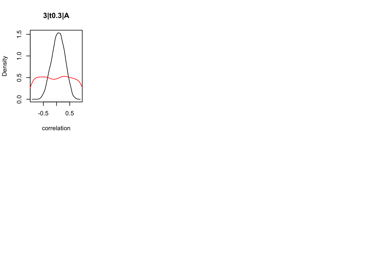
As we can see, none of the credible intervals of the correlations between the neural model and the behavioral model did not contain 0. This is not unsurprising given the low amount of behavioral trials completed. So we have to be cautious about making inference on these correlations.
8.3.4 Conclusion
Here we’ve shown how to do different types of joint models using EMC. Most of them are a proof of concept, but I hope you can see how to apply this in your own work.