Chapter 3 Separate Models of Choice or Response Time
In this chapter we detail two use cases of EMC2 for univariate data (either choice or response time). The first example uses Signal Detection Theory (SDT) to model choices from a recognition memory task. The second uses the same task, but analyses response times only (not choices), using the log normal race (LNR) model.
With our EMC2 model designs, we can now look to begin modelling the data. For this exercise, we use a sampling algorithm to estimate parameters. This chapter gives an overview of some general sampling concepts. Essentially, we test out many different parameter combinations until we find a region that is most representative of the data (for each subject). This involves calculating the likelihood on these proposed parameters and often uses Markov Chain Monte Carlo (MCMC) to gradually update the proposals to “better” regions of the parameter space (i.e., regions with the highest likelihood). Once the samples have converged and are stationary, we are said to have reached the “posterior” mode. We can then use samples from the posterior for inference (provided some other checks have been met).
Note: In both of the sections, we make very little inference from the models. This is because we only use these two models to exemplify the flexibility of the modelling code. In later lessons, we’ll use evidence accumulation models to make deeper inference about the decision making process, but for now, let’s start getting used to EMC2 functions and designs.
3.1 Signal Detection Theory
3.1.1 Theory and Model
SDT can be used to model choice. The theory posits that for a signal, we have a (normal) distribution of representations and a criteria used to make a choice. For example, take a task where people are asked to decide whether an item was seen earlier (old) or not seen previously (new), such as a recognition memory task. Using SDT, we could theorize that people have representations (distributions) of old and new stimuli which fall along a line. A criterion can then be placed on that line. If a response is made above the criterion (say where the “new” representation exists), the respondent will say “new” and vice-versa for old.
Now, this model is quite simplistic and it might be difficult to see what we gain from such a model. However, by estimating the mean (and standard deviation) of the distributions, as well as the criterion, we can gain insight into the bias that might exist. For example, the criterion could be quite low, meaning that subjects respond “new” more frequently, leading to many false alarms and a high proportion of hits. We can also see the separation between representations, where overlapping representations may indicate that it is more difficult to discriminate signal from noise. This is the basic idea behind SDT. In the following example, we show a model of SDT, using real data where participants were asked to respond to a cloud of moving dots under varying emphasis conditions (be fast, be accurate or neutral). We’ll continue using this data set throughout our examples, before showing some additional examples in later chapters.
3.1.2 Parameters
For the SDT model, EMC2 includes three parameters: threshold, mean and sd. threshold relates to the location of the criterion on our theoretical representation plane. mean relates to the means of the representations, where one mean must be held constant to avoid scaling problems (where the values could be estimated the same distance apart, but slide up and down our plane). sd relates to the variance of the representation distributions.
3.1.3 The Task
The task used here was a random dot motion task, where participants were given varying instructions preceding each trial. These instructions included “be fast”, “be accurate” or a neutral condition. The data comes from Forstmann et al. (2008).
3.1.4 EMC2 for SDT
3.1.4.1 Setup
First we need to setup the environment for EMC2. We do this by sourcing EMC2 and the model of interest. Next, we load the data. When we load the data, we remove response times, as we only use choice for the current experiment. Finally, we use only 1 subject for this example fit.
rm(list=ls())
source("emc/emc.R")
source("models/SDT/Probit/SDTgaussian.R")

print(load("Data/PNAS.RData"))
data$RT <- NA
names(data)[1]<-"subjects"
data$S <- as.factor(toupper(data$S))
data$subjects <- factor(as.character(data$subjects))
data <- data[data$subjects=="as1t",]
3.1.4.2 Design
To make a design, the following elements should be specified. There are more details on these in Chapter 2.
- “Formula factors”: The factors used in the model
- “Formula list”: Linear models for each parameter type
- Contrast list: custom contrasts to specify
- Match scoring
- Response factor levels
- Set constants
- the model.
We detail these below;
Formula Factors Here subjects is only one individual, stimuli is either right or left and emphasis is either “speed”, “accuracy” or “neutral”.
# Formula factors to be used.
Ffactors=list(subjects="as1t",S=levels(data$S),E=levels(data$E))
Formula factors For these, we need a linear model for each parameter of interest. Here we specify that mean differs across stimuli only (for now). For threshold, this varies across the latent response.
# Formula factor List.
Flist=list(mean ~ S*E, sd ~ 1, threshold ~ lR)
Response Levels For these, we need to specify the various levels of responses in the model. In this instance, we have responses ranging from 1 to 6.
# Response levels
Rlevels<-1:6
Match Scoring Here, we need to tell the model that when the stimulus is “right”, then a correct response would also be “right” and vice-versa for left stimuli, or incorrect responses.
# Match scoring
matchfun <- function(d) as.numeric(d$S) == as.numeric(d$lR)
Constants are required for scaling purposes. Here, we specify several constants for the model. To know the names of parameters, you may first need to not include this argument, make the design and then use the sampled_p_vector(design,model=NULL) function (see here) to see the parameter names.
# Constants
constants<-c(mean=0,sd=0)
Model is needed to be specified to know which model to use. These can be found in the /models folder. Here we use the probit model for SDT.
# Model
model<-probit
make_design is then used to make our SDT model design!
design <- make_design(Flist=list(mean ~ S*E, sd ~ 1, threshold ~ lR), Ffactors=list(subjects=levels(data$subjects),S=levels(data$S), E=levels(data$E)),Rlevels=levels(data$R),
                      matchfun=matchfun,
                      constants=c(mean=0,sd=0),model=probit)
3.1.4.3 Check
To check whether we specified the model correctly, lets check out the parameters and then do a quick look at profile plots and parameter recovery. First, we should check on the parameter names:
p_vector <- sampled_p_vector(design)
p_vector
## mean_SRIGHT mean_Eneutral mean_Espeed mean_SRIGHT:Eneutral
## 0 0 0 0
## mean_SRIGHT:Espeed threshold
## 0 0
## attr(,"map")
## attr(,"map")$mean
## mean mean_SRIGHT mean_Eneutral mean_Espeed mean_SRIGHT:Eneutral mean_SRIGHT:Espeed
## 1 1 0 0 0 0 0
## 2 1 0 1 0 0 0
## 3 1 0 0 1 0 0
## 4 1 1 0 0 0 0
## 5 1 1 1 0 1 0
## 6 1 1 0 1 0 1
##
## attr(,"map")$sd
## sd
## 1 1
##
## attr(,"map")$threshold
## threshold threshold_lRRIGHT
## 1 1 0
## 7 1 1Let’s now create some data using the model. For that, we first need to propose some parameter values. Note here that some of these are log transformed. The reason for this is due to transformations of the proposed parameters, which will be discussed later (see here).
p_vector[1] <- 4 #lets put the mean for the right responses at 4
p_vector[6] <-  2 #now lets try the threshold at 2. As left will be fixed at 0, this is about halfway between the mean distributions

p_vector[2:3] <- c(.2, .4) #next we're going to set the difference for neutral and speed conditions from the accuracy conditions. For neutral, we move it .2 higher, and for speed .4.
p_vector[4:5] <- c(-.8,-1.6) #Now we also include the interaction terms. Seeing as we think accuracy will be highest in the accuracy condition, we make these negative so that the distributions are closer together (more overlap)
Now that we’ve input some parameter values, we can check how this maps on to the data:
# Check mapping
mapped_par(p_vector,design)
## S E lR lM mean sd threshold
## 1 LEFT accuracy LEFT TRUE 0.0 1 2
## 2 LEFT neutral LEFT TRUE 0.2 1 2
## 3 LEFT speed LEFT TRUE 0.4 1 2
## 4 RIGHT accuracy LEFT FALSE 4.0 1 2
## 5 RIGHT neutral LEFT FALSE 3.4 1 2
## 6 RIGHT speed LEFT FALSE 2.8 1 2You can see here how we’ve made it such that the accuracy condition has the largest separation in mean parameter values. Think about how this might look (with the threshold in the middle) when plotted.
It looks like everything is correct, so now let’s simulate some data from the model:
# Simulate data
sim <- make_data(p_vector,design=design,trials=1000)
So now we have some data simulated out of the model. We can check what this data looks like, to see if the model is acting as we think it should. To do this, let’s first look at some descriptive stats:
sim$C <- sim$S==sim$R
table(sim$E,sim$C)
##
## FALSE TRUE
## accuracy 41 1959
## neutral 111 1889
## speed 279 1721# Check proportion correct
crct=sim$R==sim$S
tapply(sim$R==sim$S,sim$S,mean)## LEFT RIGHT
## 0.9573333 0.8990000# Check probability of a hit
tapply(as.numeric(sim$R)-1,sim$S,mean)## LEFT RIGHT
## 0.04266667 0.89900000# Should be about the same as this
c(pnorm(1,mean=2,sd=1),1-pnorm(1,mean=2,sd=1))## [1] 0.1586553 0.8413447Now, let’s plot the receiver operator curves (ROC) across the variables. These plots show the ROC plots, and z-scored ROC plots, for face and word stimuli (which, if you remember from above, we gave varying parameters to, so we should see some differences).
par(mfrow=c(2,2))
plot_roc(sim[sim$R=="speed",],main="Speed")
plot_roc(sim[sim$E=="speed",],zROC=TRUE,qfun=qnorm,main="Speed",lim=c(-2.5,2))
par(mfrow=c(2,2))
plot_roc(sim[sim$R=="neutral",],main="Neutral")
plot_roc(sim[sim$E=="neutral",],zROC=TRUE,qfun=qnorm,main="Speed",lim=c(-2.5,2))
par(mfrow=c(2,2))
plot_roc(sim[sim$R=="accuracy",],main="Accuracy")
plot_roc(sim[sim$E=="accuracy",],zROC=TRUE,qfun=qnorm,main="Speed",lim=c(-2.5,2))
Okay, so the data generated here looks pretty good! Now let’s check that the model is functioning correctly by using profile plots. These plots show whether the generating value for the data is located where the peak of the likelihood is (when other parameters are held constant), which we would expect to see, all going correctly. For more on profile plots, see here.
# profiles
dadm <- design_model(data=sim,design)
par(mfrow=c(2,3))
for (i in names(p_vector))
  print(profile_pmwg(pname=i,p=p_vector,p_min=p_vector[i]-.5,p_max=p_vector[i]+.5,dadm=dadm))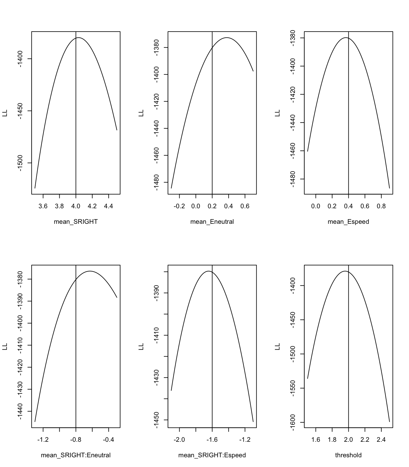
From these plots, we can see that the peak of the likelihood matches nicely with the generating values.
Finally, it’s time to make an object to be used by the sampler to do the sampling (i.e., estimate the model).
samplers <- make_samplers(sim,design,type="single")3.1.4.4 Run
Now we can do the sampling!
Note Running this code will take a significant amount of computer power (10 cpus) and may take several minutes-hours depending on the computer. We recommend sourcing the supplied examples if you are following along with the code. This can be done by saving the samples from OSF to your desktop and using; load("Desktop/osfstorage-archive/SDT/PNAS_sampled_SDT.RData")
samples <- run_burn(samplers,nstart = 100, ndiscard = 100, cores_per_chain = 1, cores_for_chains = 1, verbose_run_stage = T, step_size = 50)load("~/Desktop/emc2/models/SDT/Probit/examples/samples/PNAS_sampled_SDT.RData")3.1.4.5 Inference
Once the sampling has completed (above we only ran this for the first stage) we can move on to checking the samples. Below we show four function. plot_chains is first going to plot the chains of sampling for this model. gd_pmwg will show the Gelman-Diag statistic as an estimate of convergence for this model. plot_acfs will plot the autocorrelation across the samples. iat_pmwg will give us a measure of efficiency.
plot_chains(samples,subfilter=100)
gd_pmwg(samples,subfilter=100)
plot_acfs(samples,subfilter=100)
iat_pmwg(samples,subfilter=100)
Next, let’s plot the recovery of this model using plot_density. Here, we can see that the prior (red line) is dominated and the recovery is pretty good!
tabs <- plot_density(samples,filter="burn",subfilter=100,layout=c(2,3),pars=p_vector)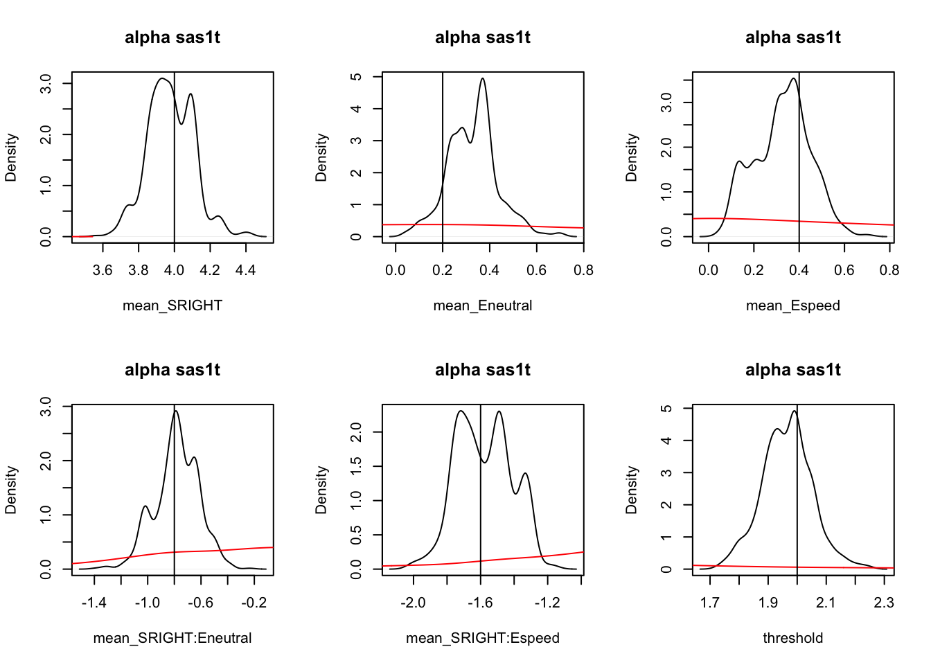
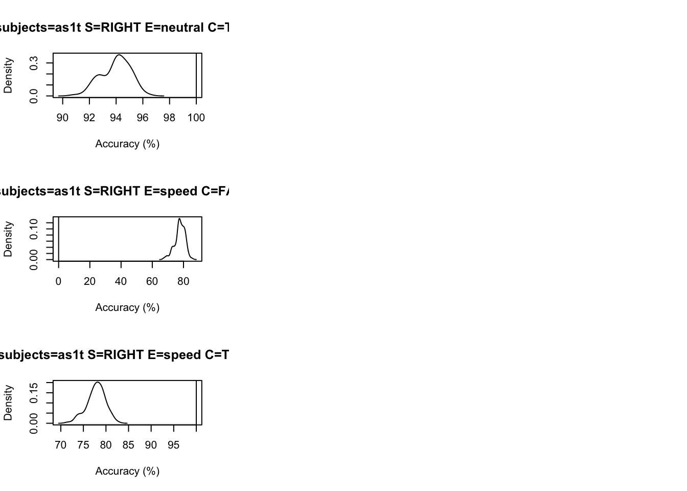
Finally, let’s make some posterior predictive data based on our samples, and then assess the accuracy of the fit. We’re just looking at accuracy of choice here, so we also need to make an “accuracy” function so that we can compare the accuracy of the “observed” data compared to what the model predicts.
ppBinary <- post_predict(samples,filter="burn",subfilter=100)## ....................................................................................................pc <- function(d) 100*mean(d$S==d$R)
# Drilling down on accuracy we see the biggest misfit is in speed for right
# responses by > 5%.
tab <- plot_fit(data=sim,pp=ppBinary,stat=pc,
stat_name="Accuracy (%)",layout=c(3,3))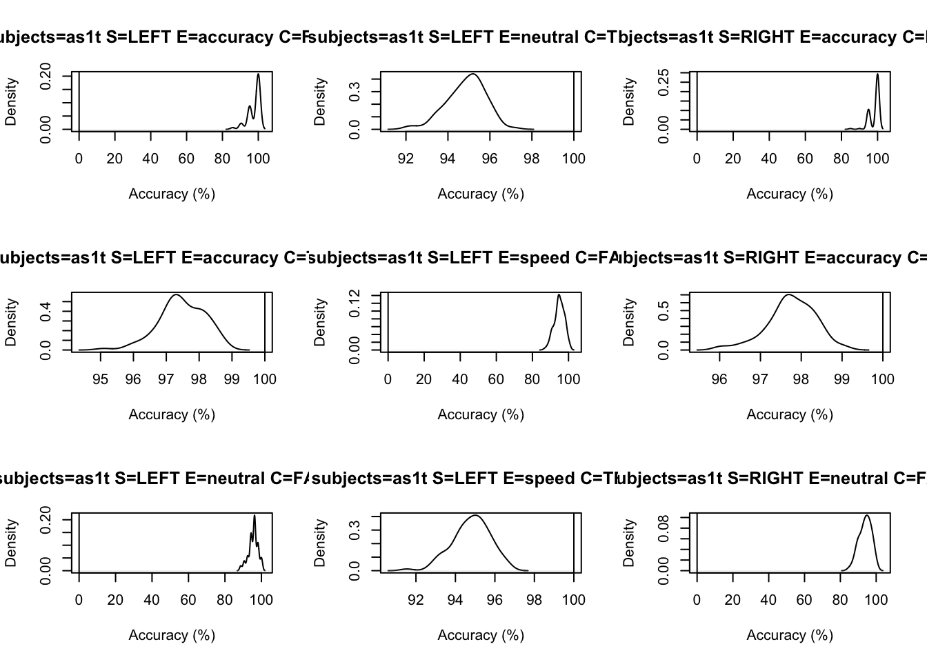
3.1.5 Conclusion
So we can see the SDT recovers well in this example! This is a nice example of a simulation and recovery exercise, where we first generate some data from the model, and then we can check to see if it recovers. Of course we could check all kinds of metrics, but as an intro to EMC2, this works nicely. To apply SDT to real data, we’ll include some additional examples later on. In the following section (and chapters), we’re going to begin introducing response times (as well as choice) into our models.
3.2 Modelling RTs with Ex-Gaussian Models
In the previous example, we only focused on choice. In decision making however, we could also look at the element of speed of choice. For these kinds of decision making experiments, we may have specific hypotheses – for example, fast responses could indicate easier trials, or more confidence from the decision maker. Here, we’re going to model the response times using an ex-gaussian model.
3.2.1 The Exponential Gaussian Distribution
The ex-gaussian distribution describes the sum of the independent normal and exponential random variables. We often use this for response time distributions as they follow a positively skewed distribution. The ex-gaussian for a random variable Z is given by Z = X + Y, where X has mean \(\mu\) and variance \(\sigma\), and Y is the exponential of the rate \(\tau\).
3.2.2 Set up
First, lets load in our data again, but this time, we’re only going to focus on RTs.
## [1] "data" "covariates"rm(list=ls())
source("emc/emc.R")
source("models/RACE/exGaussian/exGaussian.R")
# PNAS data
print( load("Data/PNAS.RData"))
dat <- data[,c("s","E","S","R","RT")]
names(dat)[c(1,5)] <- c("subjects","rt")
levels(dat$R) <- levels(dat$S)Next we’re going to modify the data to only include the correct responses. Often descriptive analyses with the ExGaussian are done only on correct responses.
dat <- dat[dat$S==dat$R,]Next, we’re going to design the model, similar to how we did for SDT. Here, we fit the model to individual design cells. This will be explained in later lessons, for now though, just note this enables us to fit an 18 parameter model, with separate mu, sigma and tau estimates for each cell of the design (i.e., across all conditions).
se <- function(d) {factor(paste(d$S,d$E,sep="_"),levels=
  c("left_accuracy","right_accuracy","left_neutral","right_neutral","left_speed","right_speed"))}

designEXG <- make_design(
  Ffactors=list(subjects=levels(dat$subjects),S=levels(dat$S),E=levels(dat$E)),
  Rlevels=levels(dat$R),
  Clist=list(SE=diag(6)),
  Flist=list(mu~0+SE,sigma~0+SE,tau~0+SE),
  Ffunctions = list(SE=se),
  model=exGaussian)
## mu_SEleft_accuracy mu_SEright_accuracy mu_SEleft_neutral
## 0 0 0
## mu_SEright_neutral mu_SEleft_speed mu_SEright_speed
## 0 0 0
## sigma_SEleft_accuracy sigma_SEright_accuracy sigma_SEleft_neutral
## 0 0 0
## sigma_SEright_neutral sigma_SEleft_speed sigma_SEright_speed
## 0 0 0
## tau_SEleft_accuracy tau_SEright_accuracy tau_SEleft_neutral
## 0 0 0
## tau_SEright_neutral tau_SEleft_speed tau_SEright_speed
## 0 0 0
## attr(,"map")
## attr(,"map")$mu
## mu_SEleft_accuracy mu_SEright_accuracy mu_SEleft_neutral mu_SEright_neutral
## 1 1 0 0 0
## 39 0 0 1 0
## 77 0 0 0 0
## 20 0 1 0 0
## 58 0 0 0 1
## 96 0 0 0 0
## mu_SEleft_speed mu_SEright_speed
## 1 0 0
## 39 0 0
## 77 1 0
## 20 0 0
## 58 0 0
## 96 0 1
##
## attr(,"map")$sigma
## sigma_SEleft_accuracy sigma_SEright_accuracy sigma_SEleft_neutral
## 1 1 0 0
## 39 0 0 1
## 77 0 0 0
## 20 0 1 0
## 58 0 0 0
## 96 0 0 0
## sigma_SEright_neutral sigma_SEleft_speed sigma_SEright_speed
## 1 0 0 0
## 39 0 0 0
## 77 0 1 0
## 20 0 0 0
## 58 1 0 0
## 96 0 0 1
##
## attr(,"map")$tau
## tau_SEleft_accuracy tau_SEright_accuracy tau_SEleft_neutral tau_SEright_neutral
## 1 1 0 0 0
## 39 0 0 1 0
## 77 0 0 0 0
## 20 0 1 0 0
## 58 0 0 0 1
## 96 0 0 0 0
## tau_SEleft_speed tau_SEright_speed
## 1 0 0
## 39 0 0
## 77 1 0
## 20 0 0
## 58 0 0
## 96 0 1We can see this from the vector of parameters output above. For each parameter (\(\mu\), \(\sigma\) and \(\tau\)) this design gives us 6 parameters to estimate. These 6 parameters represent the cell coded design, where each combination of conditions across the factors of “stimuli” and “emphasis” have a parameter.
3.2.3 Run sampling
Note Running this code will take a significant amount of computer power (10 cpus) and may take several minutes-hours depending on the computer. We recommend sourcing the supplied examples if you are following along with the code. This can be done by saving the samples from OSF to your desktop and using; load("Desktop/osfstorage-archive/ExGauss/sPNAS_exg.RData")
samplers <- make_samplers(dat,designEXG,type="standard",rt_resolution=.02)

rm(list=ls())
source("emc/emc.R")
source("models/RACE/exGaussian/exGaussian.R")
run_emc("sPNAS_exg.RData",cores_per_chain=10)
# Add samples to get get 2000 converged after first 500.
run_emc("sPNAS_exg.RData",cores_per_chain=10,nsample=1500)
# Get posterior predictives
load("sPNAS_exg.RData")
pp <- post_predict(samplers,n_cores=19,subfilter=500)
save(samplers,pp,file="sPNAS_exg.RData")
We’ve already run this for you, so you can source the samples from the OSF link above.
load("~/Desktop/emc2/models/RACE/exGaussian/examples/samples/sPNAS_exg.RData")3.2.4 Check the run
Next, we want to use the function below to run through a variety of model checks. These are typical graphical model checks. Can you see anything of note from these chain plots? We’ll go into more detail in later chapters regarding what to look out for and how to overcome such issues.
check_run(samplers,layout=c(3,6),width=12,subfilter=500)3.2.5 Check model fit
Now we can check the model fit. Here, posterior prediction (done above) did not use the first 500 samples, so inference is based on the last 2000 iterations across the three chains. We do this to ensure we are sampling from the posterior region when generating data (and doing inference). See the results from the check_run function to assess the stationarity of the sampling and evaluate if we are likely to be in the posterior mode.
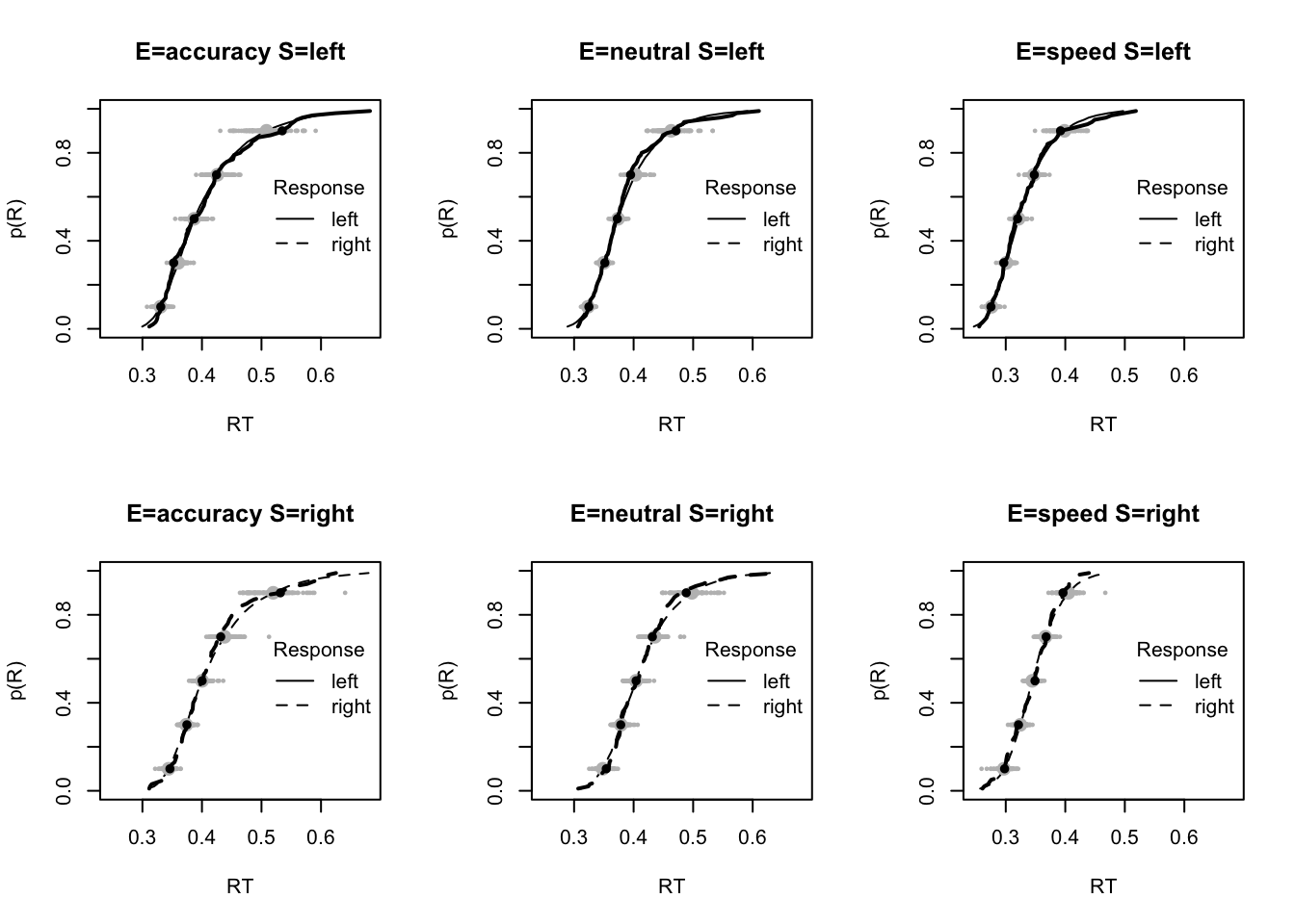
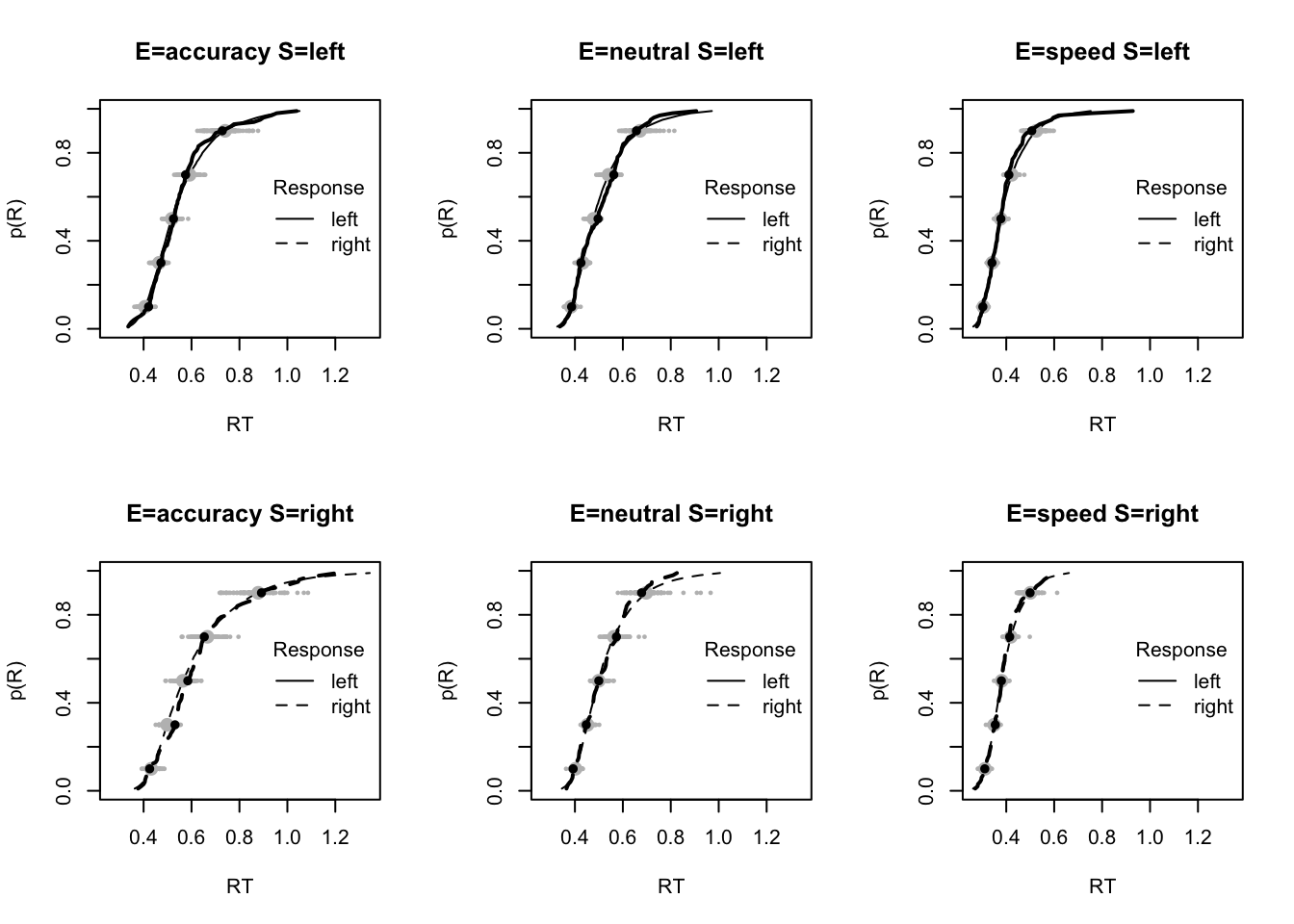
plot_fit(dat,pp,layout=c(2,3),factors=c("E","S"),lpos="right",xlim=c(.25,1.5))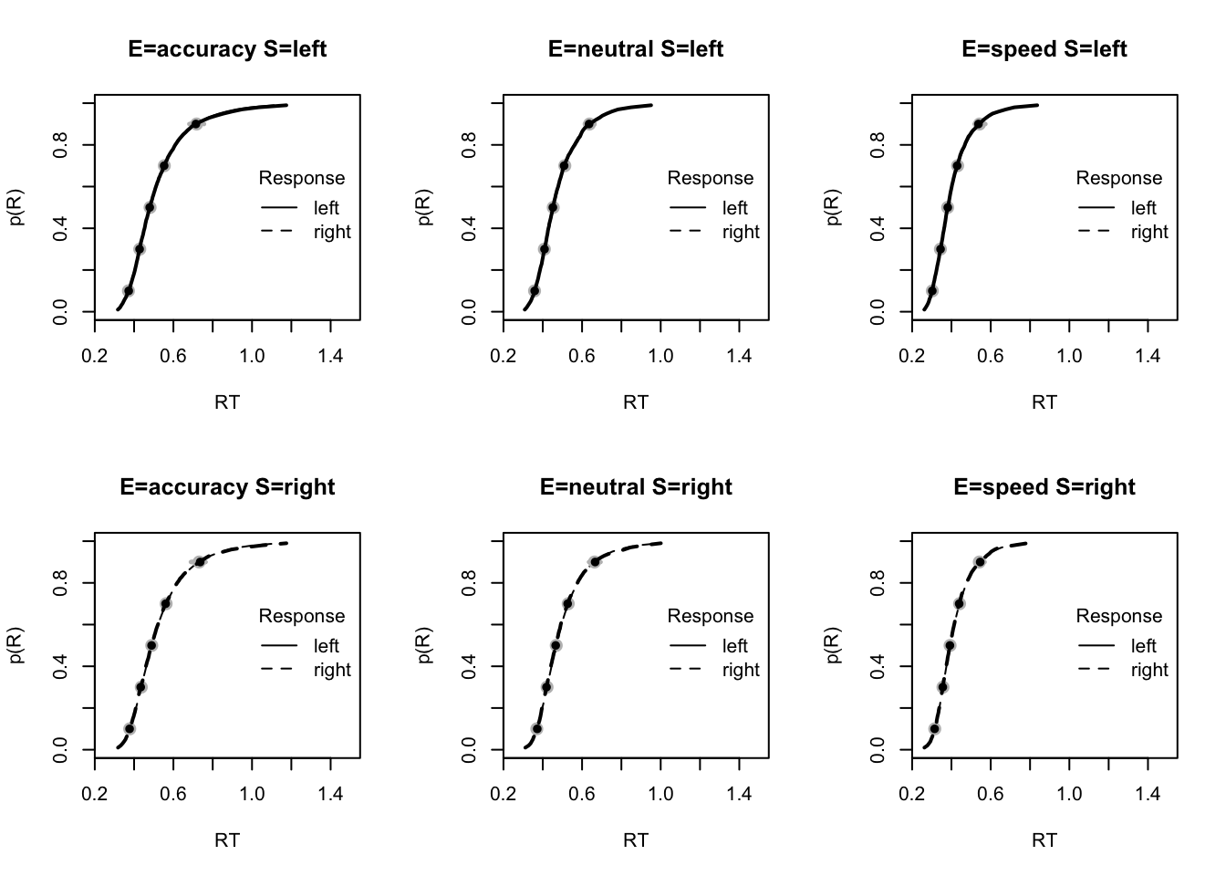
plot_fits(dat,pp,layout=c(2,3),lpos="right")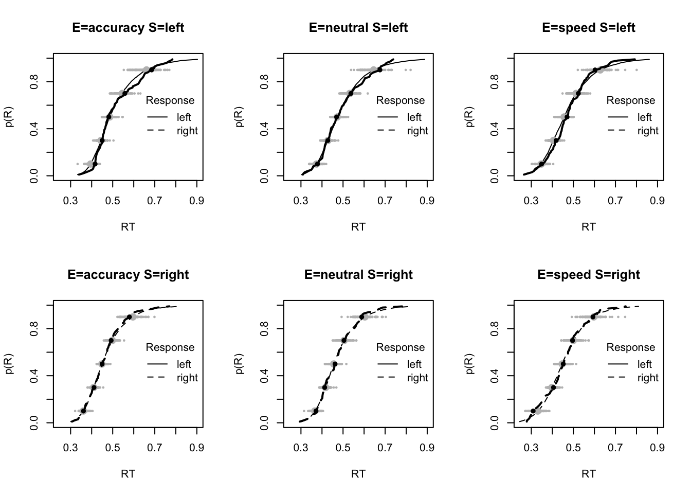
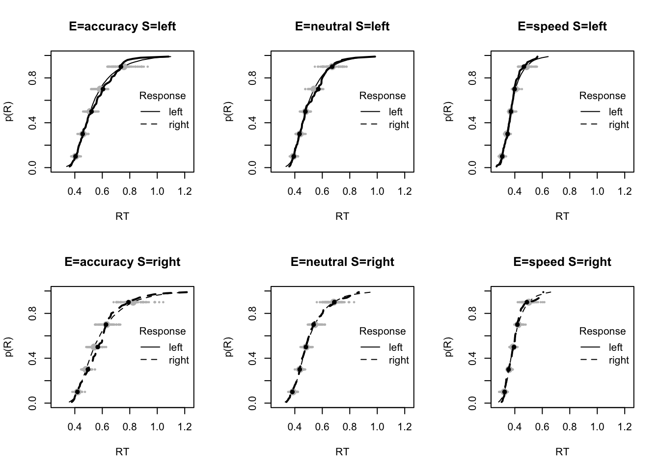
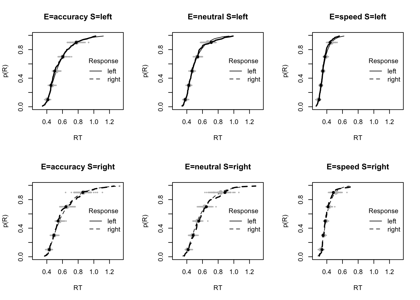
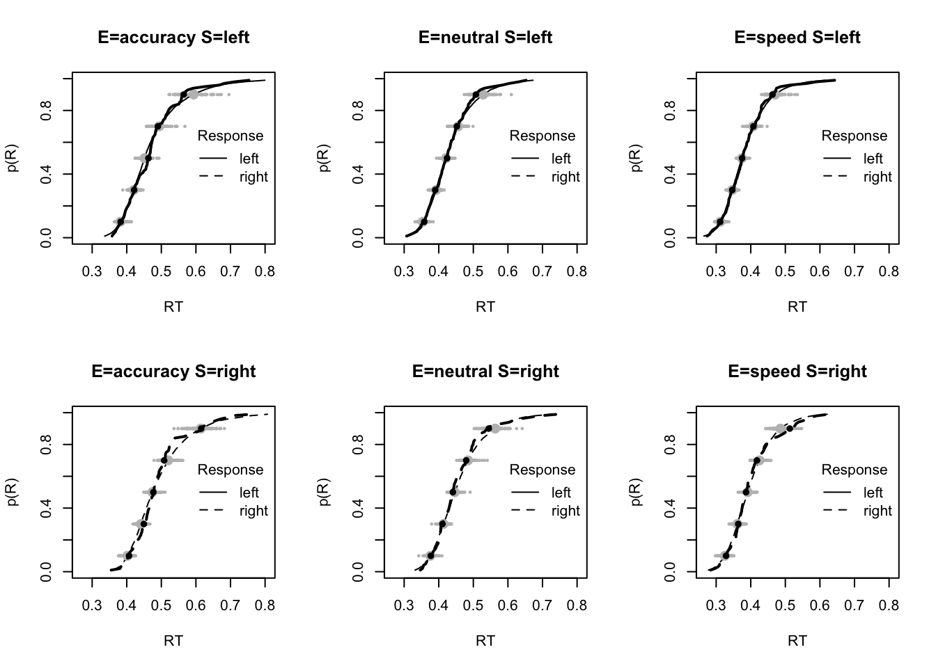
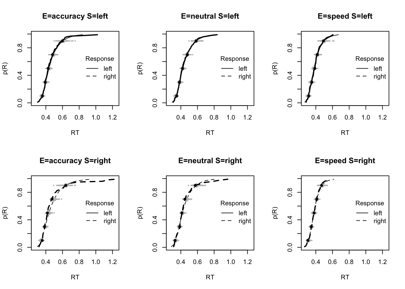
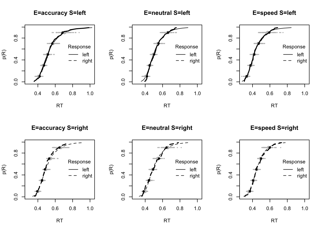

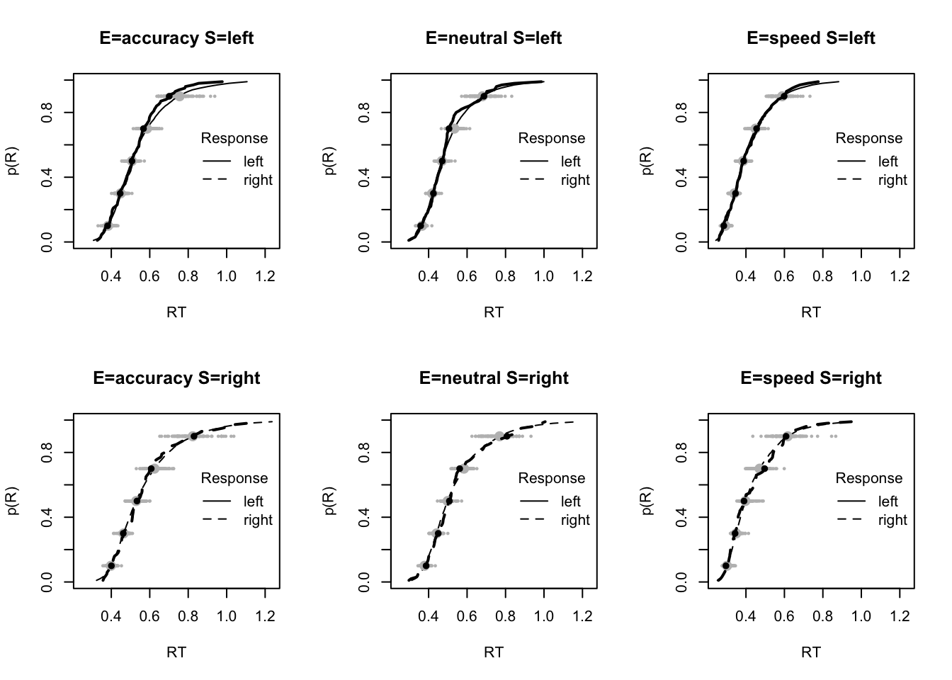
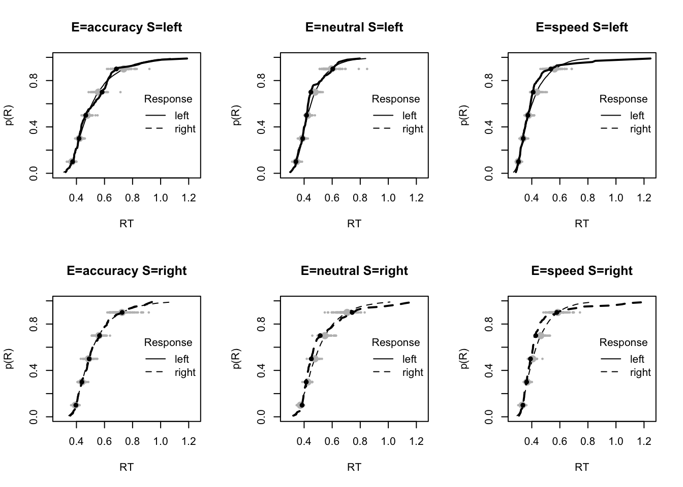
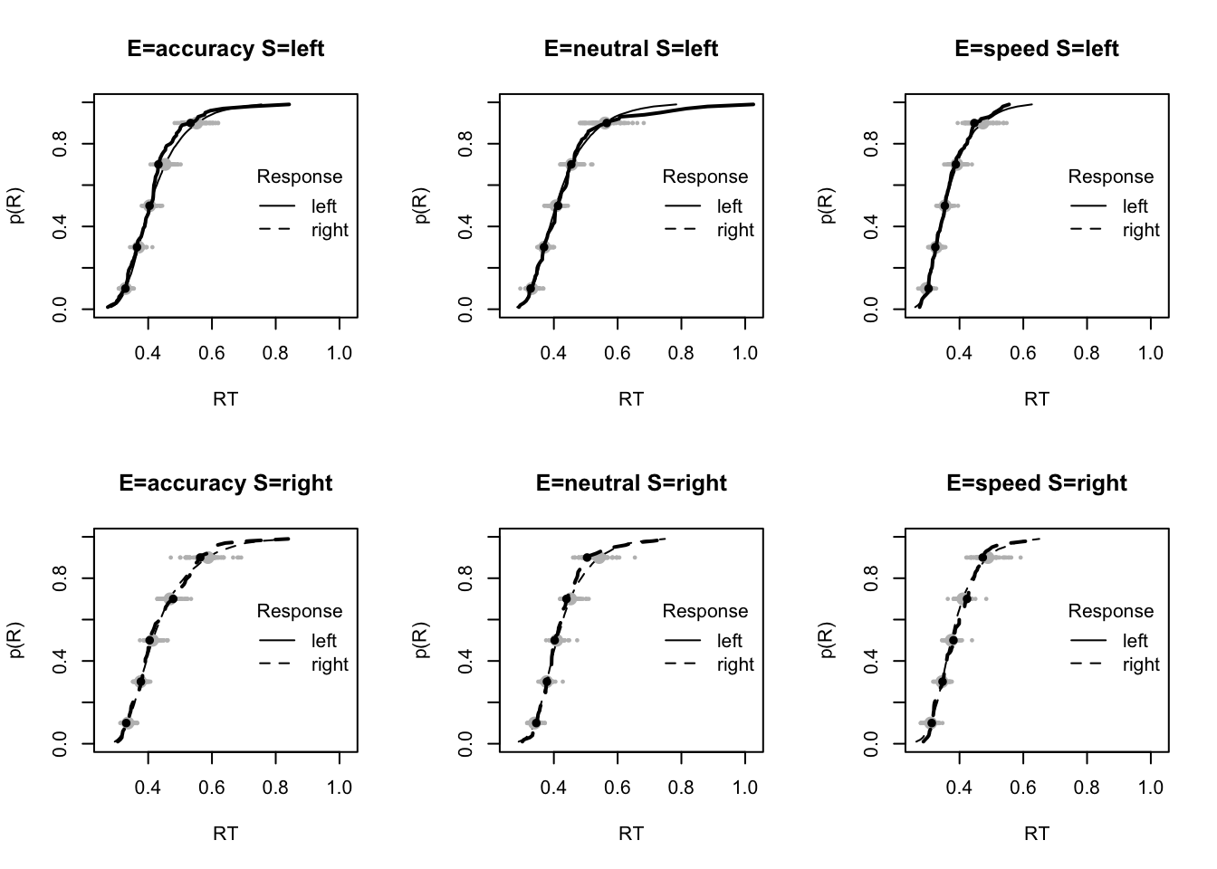
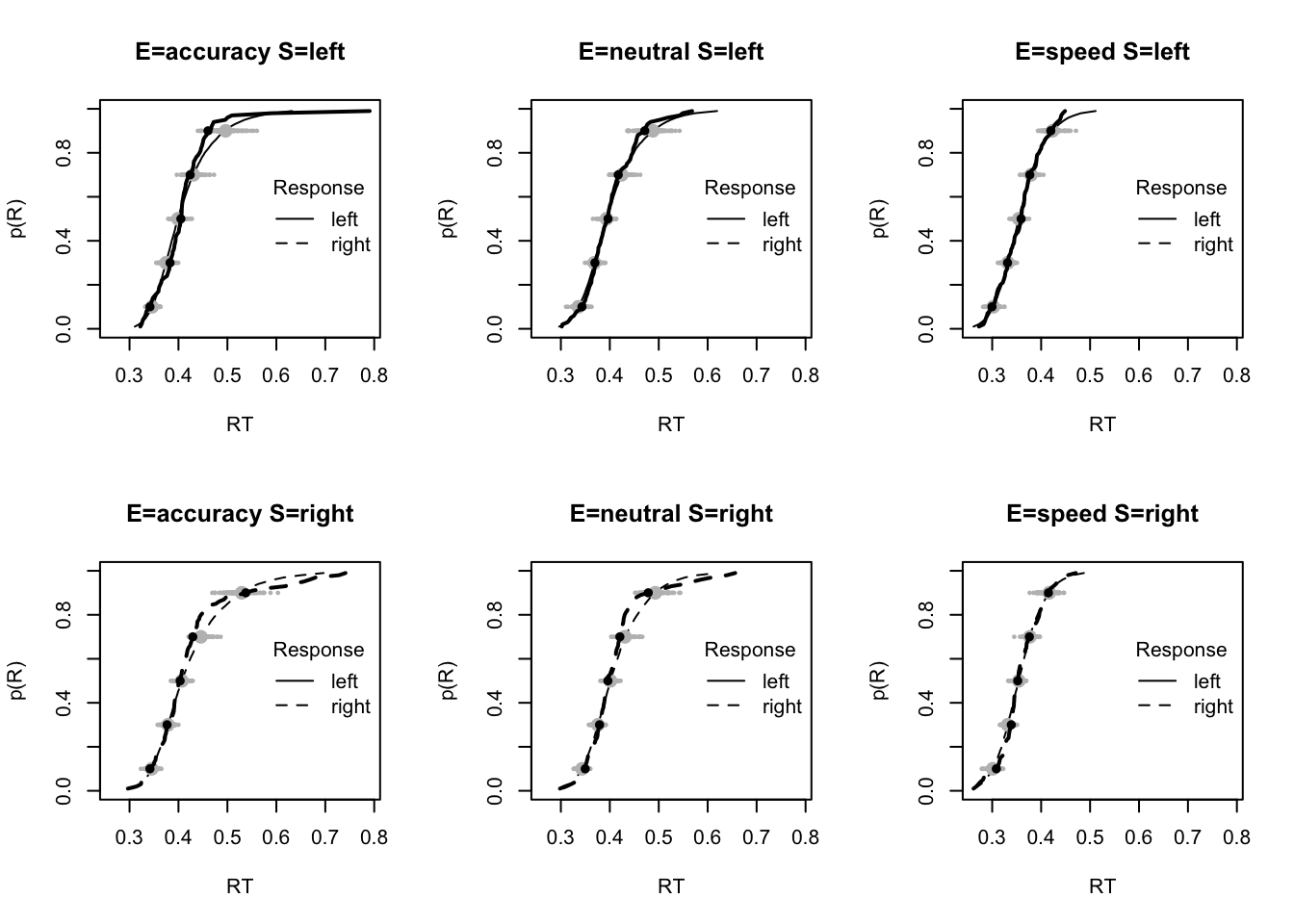
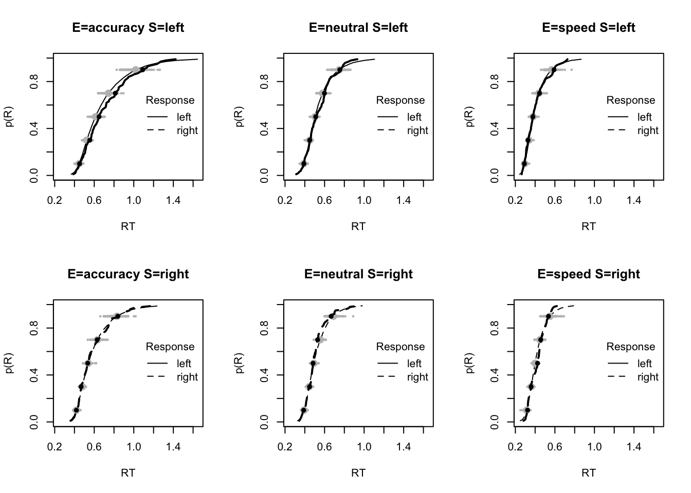
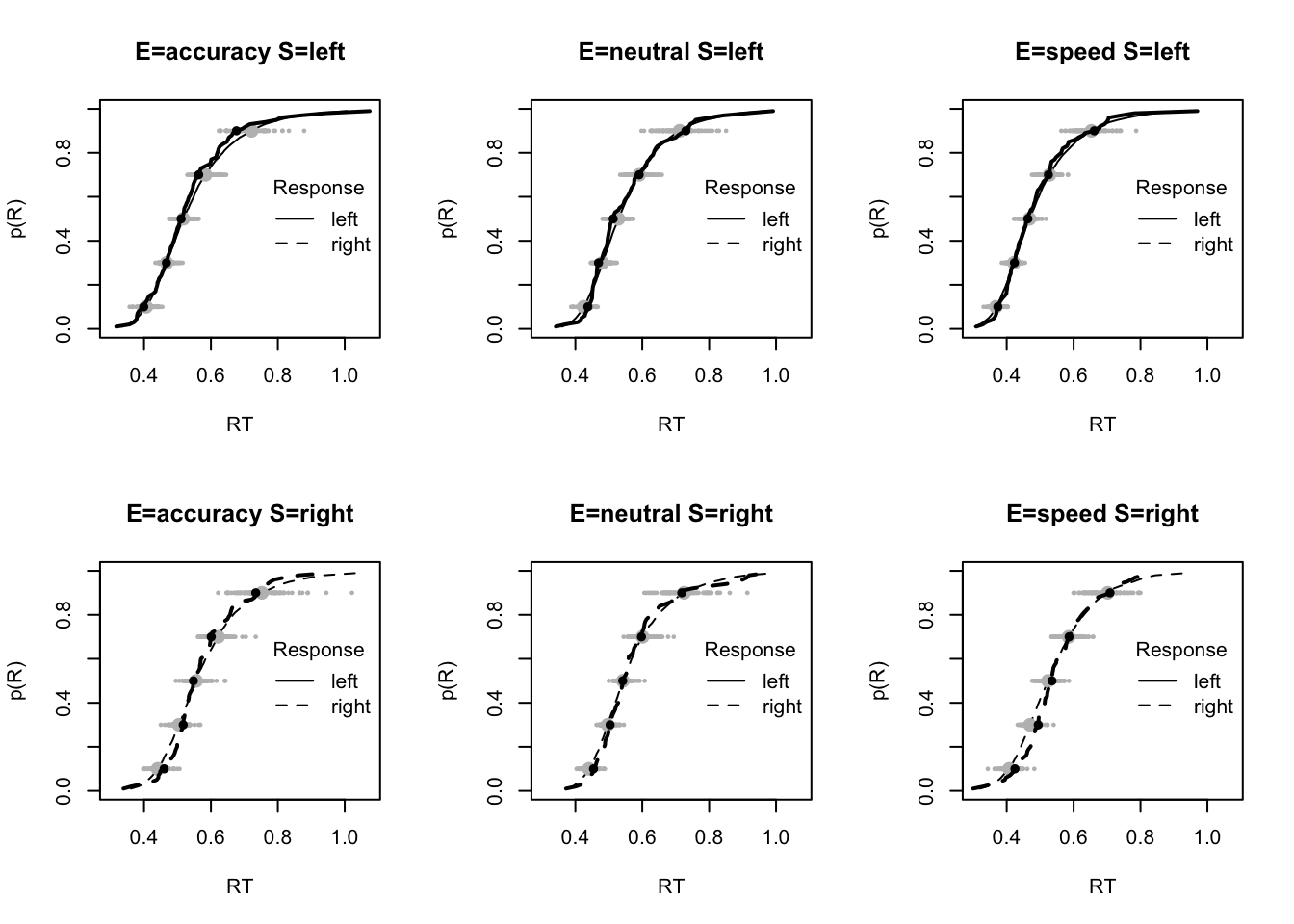
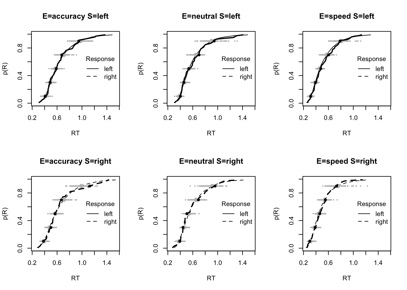
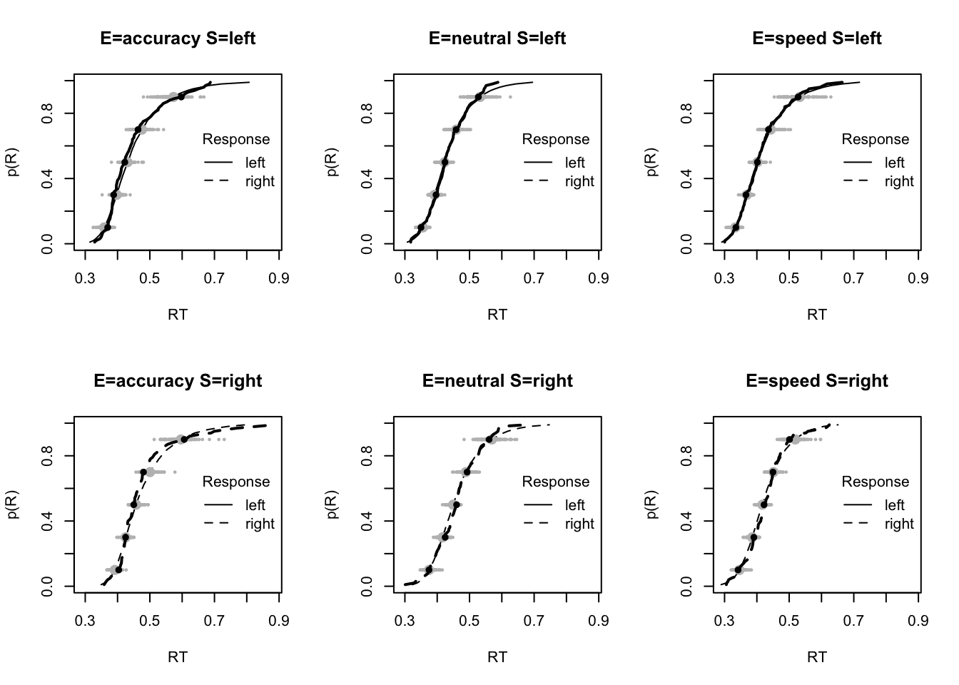
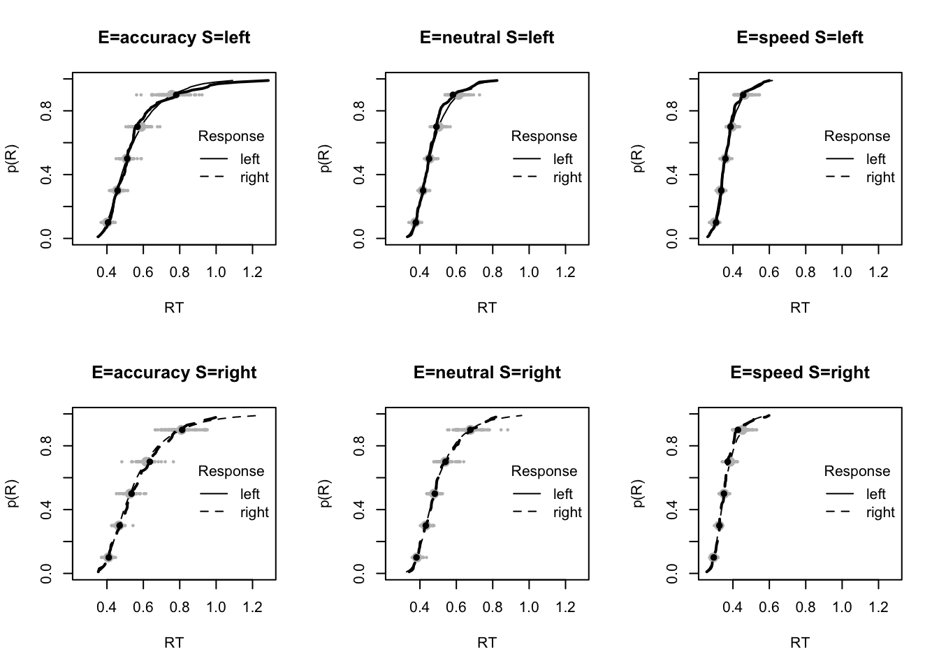
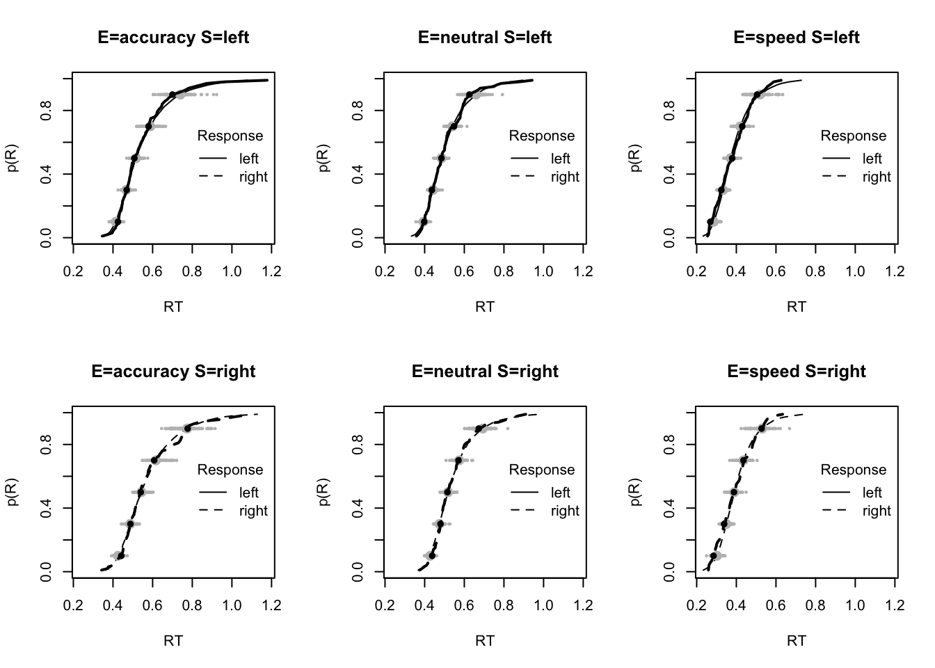
The code below shows some further plots (which you can run for yourself) highlighting that the model very accurately fits the data. In these examples, we show the RT fit across the mean, 10 and 90% quantiles, and for the standard deviation of the observed vs expected (model predicted).
tab <- plot_fit(dat,pp,layout=c(2,3),factors=c("E","S"),
         stat=function(d){mean(d$rt)},stat_name="Mean RT (s)",xlim=c(0.375,.625))
tab <- plot_fit(dat,pp,layout=c(2,3),factors=c("E","S"),xlim=c(0.275,.4),
         stat=function(d){quantile(d$rt,.1)},stat_name="10th Percentile (s)")
tab <- plot_fit(dat,pp,layout=c(2,3),factors=c("E","S"),xlim=c(0.525,.975),
         stat=function(d){quantile(d$rt,.9)},stat_name="90th Percentile (s)")
tab <- plot_fit(dat,pp,layout=c(2,3),factors=c("E","S"),
         stat=function(d){sd(d$rt)},stat_name="SD (s)",xlim=c(0.1,.355))
3.2.6 Inference
For inference, let’s first check and see whether the parameters moved away from the prior using the information in the data. Here, we show code for both the credible intervals on the sampled and natural scale, however, we only plot those on the natural scale (i.e., the scale used by the model). We can see from these the prior (red line) is well dominated by the posterior group level samples;
ci <- plot_density(samplers,layout=c(3,6),selection="mu",subfilter=500)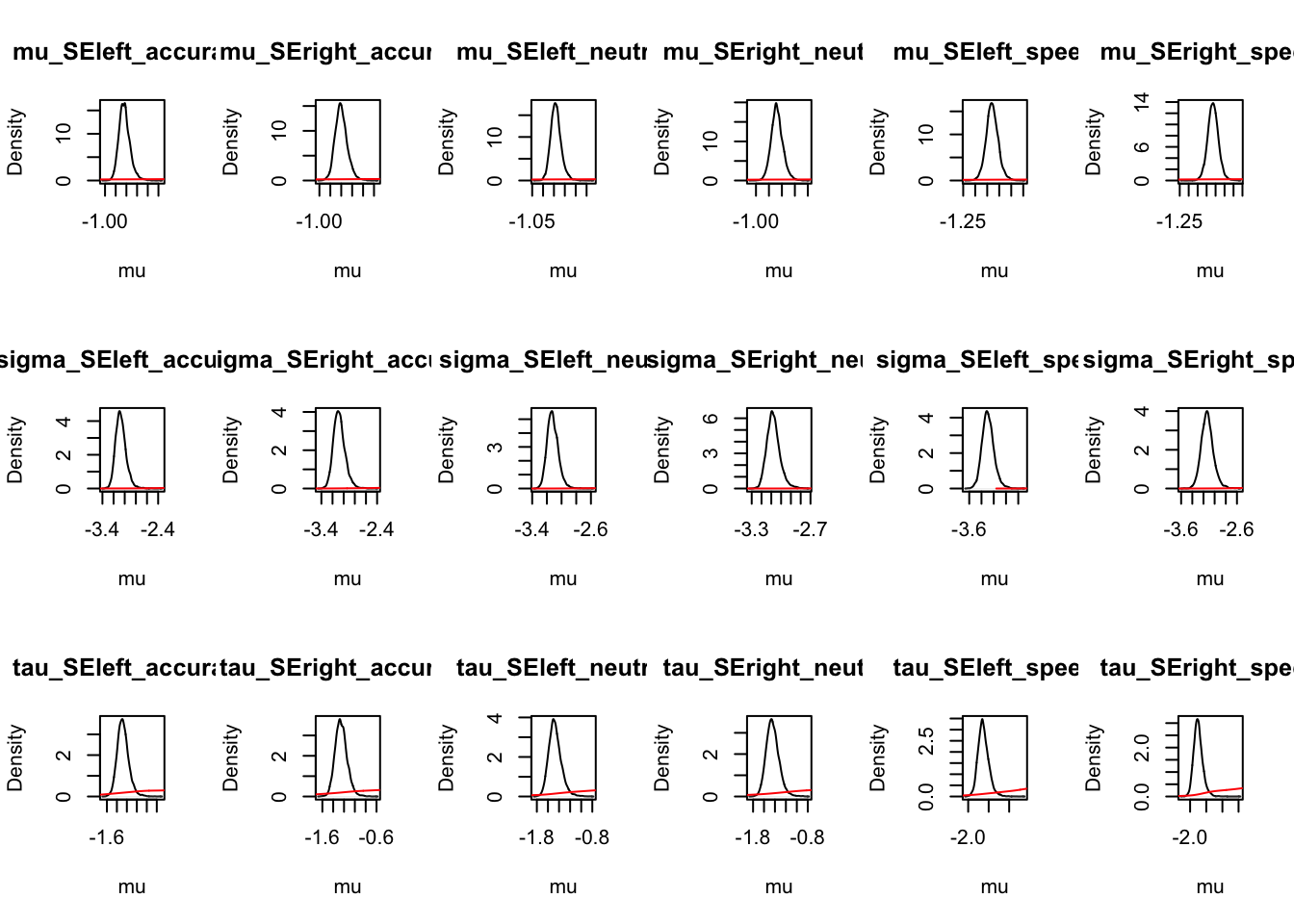
ci_mapped <- plot_density(samplers,layout=c(3,6),subfilter=500,
                                        selection="mu",mapped=TRUE)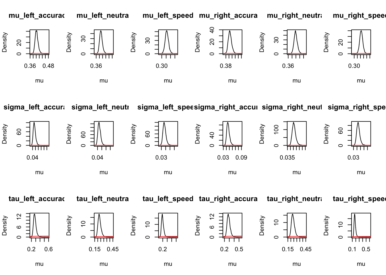
#round(ci,2)
round(ci_mapped,2)
## mu_left_accuracy mu_left_neutral mu_left_speed mu_right_accuracy
## 2.5% 0.39 0.37 0.31 0.39
## 50% 0.40 0.39 0.32 0.41
## 97.5% 0.43 0.41 0.34 0.43
## mu_right_neutral mu_right_speed sigma_left_accuracy sigma_left_neutral
## 2.5% 0.38 0.33 0.04 0.04
## 50% 0.40 0.34 0.05 0.04
## 97.5% 0.42 0.37 0.06 0.05
## sigma_left_speed sigma_right_accuracy sigma_right_neutral sigma_right_speed
## 2.5% 0.03 0.04 0.04 0.04
## 50% 0.04 0.05 0.05 0.04
## 97.5% 0.05 0.06 0.05 0.06
## tau_left_accuracy tau_left_neutral tau_left_speed tau_right_accuracy
## 2.5% 0.23 0.19 0.16 0.23
## 50% 0.28 0.23 0.19 0.28
## 97.5% 0.36 0.30 0.26 0.36
## tau_right_neutral tau_right_speed
## 2.5% 0.19 0.14
## 50% 0.23 0.17
## 97.5% 0.30 0.24Next, the p_test function does a parameter test, similar to a t-test, to help evaluate differences between parameters. Which of these are the most surprising? First let’s look at the skew of the distribution;
# skew: accuracy > neutral > speed
p_test(x=samplers,mapped=TRUE,x_name="left skew: accuracy - speed",
  x_fun=function(x){x["tau_left_accuracy"]-x["tau_left_speed"]})
## left skew: accuracy - speed mu
## 2.5% 0.03 NA
## 50% 0.08 0
## 97.5% 0.13 NA
## attr(,"less")
## [1] 0.005p_test(x=samplers,mapped=TRUE,x_name="right skew: accuracy - speed",
x_fun=function(x){x["tau_right_accuracy"]-x["tau_right_speed"]})## right skew: accuracy - speed mu
## 2.5% 0.06 NA
## 50% 0.11 0
## 97.5% 0.17 NA
## attr(,"less")
## [1] 0.001p_test(x=samplers,mapped=TRUE,x_name="left skew: accuracy - neutral",
x_fun=function(x){x["tau_left_accuracy"]-x["tau_left_neutral"]})## left skew: accuracy - neutral mu
## 2.5% 0.01 NA
## 50% 0.05 0
## 97.5% 0.09 NA
## attr(,"less")
## [1] 0.013p_test(x=samplers,mapped=TRUE,x_name="right skew: accuracy - neutral",
x_fun=function(x){x["tau_right_accuracy"]-x["tau_right_neutral"]})## right skew: accuracy - neutral mu
## 2.5% 0.01 NA
## 50% 0.05 0
## 97.5% 0.09 NA
## attr(,"less")
## [1] 0.011Next, let’s look at the means for each condition. Does anything stand out here? Think about what these could mean;
# Mean RT: accuracy > neutral > speed
p_test(x=samplers,mapped=TRUE,x_name="left mean: accuracy - speed",
  x_fun=function(x){sum(x[c("mu_left_accuracy","tau_left_accuracy")]) -
                    sum(x[c("mu_left_speed","tau_left_speed")])})
## left mean: accuracy - speed mu
## 2.5% 0.10 NA
## 50% 0.16 0
## 97.5% 0.23 NA
## attr(,"less")
## [1] 0p_test(x=samplers,mapped=TRUE,x_name="right mean: accuracy - speed",
x_fun=function(x){sum(x[c("mu_right_accuracy","tau_right_accuracy")]) -
mean(x[c("mu_right_speed","tau_right_speed")])})## right mean: accuracy - speed mu
## 2.5% 0.38 NA
## 50% 0.43 0
## 97.5% 0.51 NA
## attr(,"less")
## [1] 0p_test(x=samplers,mapped=TRUE,x_name="left mean: accuracy - neutral",
x_fun=function(x){sum(x[c("mu_left_accuracy","tau_left_accuracy")]) -
sum(x[c("mu_left_neutral","tau_left_neutral")])})## left mean: accuracy - neutral mu
## 2.5% 0.02 NA
## 50% 0.06 0
## 97.5% 0.11 NA
## attr(,"less")
## [1] 0.004p_test(x=samplers,mapped=TRUE,x_name="right mean: accuracy - neutral",
x_fun=function(x){sum(x[c("mu_right_accuracy","tau_right_accuracy")]) -
sum(x[c("mu_right_neutral","tau_right_neutral")])})## right mean: accuracy - neutral mu
## 2.5% 0.02 NA
## 50% 0.06 0
## 97.5% 0.10 NA
## attr(,"less")
## [1] 0.005We could also check out SD’s using the code below;
# SD R: accuracy > neutral > speed
p_test(x=samplers,mapped=TRUE,x_name="left SD: accuracy - speed",
  x_fun=function(x){sqrt(sum(x[c("mu_left_accuracy","tau_left_accuracy")]^2)) -
                    sqrt(sum(x[c("mu_left_speed","tau_left_speed")]^2))})

p_test(x=samplers,mapped=TRUE,x_name="right SD: accuracy - speed",
  x_fun=function(x){sqrt(sum(x[c("mu_right_accuracy","tau_right_accuracy")]^2)) -
                    sqrt(sum(x[c("mu_right_speed","tau_right_speed")]^2))})

p_test(x=samplers,mapped=TRUE,x_name="left SD: accuracy - neutral",
  x_fun=function(x){sqrt(sum(x[c("mu_left_accuracy","tau_left_accuracy")]^2)) -
                    sqrt(sum(x[c("mu_left_neutral","tau_left_neutral")]^2))})

p_test(x=samplers,mapped=TRUE,x_name="right SD: accuracy - neutral",
  x_fun=function(x){sqrt(sum(x[c("mu_right_accuracy","tau_right_accuracy")]^2)) -
                    sqrt(sum(x[c("mu_right_neutral","tau_right_neutral")]^2))})
3.2.7 Conclusion
Here we’ve briefly shown the Ex-Gaussian model for correct choice RTs. In the next lesson, we’ll incorporate both choice (correct and error) and RTs into the one model. In these examples we will also give much greater depth to inference and checking, so that you can feel confident to start designing your own models for your data.