Chapter 8 Calibration and Sensitivity

Many scientific phenomena are studied with mathematical (i.e., computer) models and field experiments simultaneously. Real experiments are expensive, and for this and other reasons (ethics, lack of materials/infrastructure, etc.) limited configurations can be entertained. Computer simulations are lots cheaper, but usually not so cheap as to allow infinite exploration of configuration space(s). Plus simulations usually idealize reality, contributing bias, and engage more “knobs”, or tuning parameters, than can be controlled or even known in the field.

So the goal in the first part of this chapter is to build an apparatus that can harmonize two data types, computer simulated and field observation, for the purpose of learning about/predicting the real underlying process, or possibly optimizing some aspect of it. We want to learn about any discrepancies, or bias, between computer model and field data; learn best settings of the computer model’s knobs; meta-model/emulate computer model runs as a surrogate for new predictions, while compensating for its bias relative to reality as measured in the field. Ideally those predictions will offer a full accounting of uncertainty, for all things being estimated at all levels.

What’s meant by full, and what’s reasonable pragmatically, is always a matter of perspective. Uncertainty quantification (UQ) is a loaded term from the applied math/numerical analysis community. A lot of UQ focuses on understanding distributions of outputs, or observables from a process, as a function of uncertain or random inputs. Most applications amount to uncertainty propagation. A key component of that is understanding how inputs affect outputs when layers of fitted models are used, like GPs for surrogates and additionally as models of discrepancy in the calibration context. So the second half of the chapter takes a diversion to detail estimating main effects and sensitivity indices for GPs and related nonparametric predictors.

These two topics, calibration and sensitivity, could easily stand alone in their own chapter(s). See Chapters 7–8 of Santner, Williams, and Notz (2018). Sensitivity analysis has filled entire textbooks, although the context of those presentations is different. My aim in combining them here is to frame them as two important applications of GP surrogates where UQ, i.e., faithful propagation of uncertainty, is key.

8.1 Calibration

Computer model calibration juggles three processes. Real process \(R\) represents an ideal, depicting unknown dynamics of phenomena under study. The goal is to learn as much as possible about \(R\) through mathematical modeling, computer and physical experimentation, which leads us to the other two processes. Field \(F\) is where a physical experiment observing \(R\) takes place. Computer model \(M\) implements/solves a mathematical model that idealizes \(R\).

Let \(Y^F(x)\) denote a field observation under \(m_x\)-dimensional conditions \(x\), and \(y^R(x)\) denote the real output under condition \(x\). Assume \(R\) and \(F\) are related as follows.

\[ Y^F(x) = y^R(x) + \varepsilon, \quad \mbox{ where } \quad \varepsilon \stackrel{\mathrm{iid}}{\sim} \mathcal{N}(0, \sigma_\varepsilon^2) \]

This isn’t much different from typical modeling apparatuses where observations are corrupted by independent and identically distributed idiosyncratic Gaussian noise. Considering the expense of setting up a physical experiment in the field, we presume that only a small number \(n_F\) of field observations \(Y_{n_F}\) are available at \(x\) locations \(X_{n_F}\). Sometimes it’s easier to obtain repeated observations under a single setting \(x\), rather than changing \(x\) which may involve manually re-configuring a complex system, so \(n_F\) may embed a nontrivial degree of replication. Replicates can be helpful for separating signal from noise, especially when \(\sigma_\varepsilon^2\) is large. That is, the number of unique settings in \(X_{n_F}\) may be many fewer than \(n_F\). Chapter 10 considers modeling and design under replication in more detail. For now let me simply remark that replication is common in field experiments, and computer model calibration settings are no different. However this detail is largely ignored for the remainder of the chapter.

Let \(y^M(x, u)\) denote output from a computer model run under conditions \(x\) and tuning or calibration parameters \(u\). We shall presume that \(y^M(\cdot,\cdot)\) is deterministic to simplify the following discussion. There’s no reason why stochastic simulation must be precluded by the framework, however such setups are far less well investigated in the literature. Inputs \(x\) to computer model \(y^M(x, u)\) coincide with \(x\)’s from the field experiment(s). Inputs \(u\), in dimension \(m_u\), represent any aspect of \(M\) which can’t be controlled in \(F\) and/or are unknown in \(R\). It’s quite typical for a mathematical model, or its computer implementation, to have more knobs than can be controlled in the field. Example \(u\) coordinates may arise from an artificial aspect of computer implementation, like mesh size. Or they might have real physical meaning, like acceleration due to gravity, which is not known (precisely enough) to be recorded in the field. Some practitioners make a distinction between the two, calling the former a tuning parameter (omitting from probabilistic modeling enterprises), and treating only the latter as a calibration parameter \(u\). I’ll be lazy by using those two terms interchangeably and modeling in a unified fashion.

The goal is to study the relationship between the computer model \(y^M(x, u)\), its fine-tuning through \(u\), and the field \(Y^F(x)\) as a means of learning about real phenomena \(y^R(x)\). In this way, calibration is an example or generalization of a statistical inverse problem. Which it is – example or generalization – depends on your perspective. Inverse problems emphasize learning \(u\), attempting to attribute causal links between unknown factors in a simulation and empirical, physical observation. Calibration is more ambitious in its attempt to synthesize multiple information sources and to assimilate functional relationships through an acknowledgment of bias between computer simulation and field observation. Often such assimilation is at odds with the establishment of causal links, however, and can suffer from confounding and identification issues.

Although there are many ways you could imagine undertaking such an analysis, one has percolated to the top as canonical: the Kennedy and O’Hagan framework. Another approach, called history matching, is a popular alternative (Craig et al. 1996; Vernon, Goldstein, and Bower 2010; Williamson et al. 2013). History matching is a more hands-on process, as is perhaps exemplified by the flow diagram found at that link. Although there’s much to recommend a more careful approach to marrying disparate sources of information, the presentation below emphasizes a more easily automated Kennedy and O’Hagan alternative.

8.1.1 Kennedy and O’Hagan framework

Kennedy and O’Hagan (2001) proposed a Bayesian framework for coupling \(M\) and \(F\). KOH, hereafter, represent a real process \(R\) as the computer model output at the best setting of calibration parameters, \(u^\star\), plus a discrepancy term acknowledging that there can be systematic disagreement between model and truth.

\[ \begin{aligned} y^R(x) &= y^M(x, u^\star) + b(x) \\ \mbox{so that } \quad Y^F(x) &= y^M(x,u^\star) + b(x) + \varepsilon \end{aligned} \]

The quantity \(b(\cdot)\) is a functional discrepancy, or bias correction. Although I may shorten and casually refer to \(b(\cdot)\) as “bias”, the actual bias (which is a property of \(M\) not \(R\)) would actually work out to

\[ -b(x) = y^M(x, u^\star) - y^R(x). \]

The point here is that a computer model has systematic imperfections, even under its best tuning \(u^\star\), but KOH specify an a priori belief that reasonable correction can be learned through \(b(\cdot)\). Errors \(\varepsilon\) are independent zero-mean Gaussian with variance \(\sigma_\varepsilon^2\).

Altogether, unknowns are \(u^\star\), \(\sigma_\varepsilon^2\), and discrepancy \(b(\cdot)\). KOH emphasized Bayesian inference, particularly averaging over trade-offs between calibration values \(u\) and discrepancies \(b(\cdot)\) under a GP prior. Known information or restrictions on \(u\)-values can be specified through prior \(p(u)\). Otherwise a uniform prior (over a finite domain) can be used. Often, and especially when little prior information is available on \(u\), a regularizing prior with mass somewhat more concentrated on a default or midway value can prevent over-concentration of posterior density on boundary settings. Reference priors for \(\sigma_\varepsilon^2\) are typical (Berger, De Oliveira, and Sansó 2001). KOH utilized a GP specification with linear mean for \(b(\cdot)\), but the presentation here considers a zero-mean for simplicity and for consistency with GP treatments elsewhere in this monograph. Results analogous to those from a homework exercise in §5.5 offer ready extension.

If evaluating the computer model is fast, then inference (Bayesian or otherwise) is made rather straightforward via residuals between computer model outputs and field observations at \(n_F\) field locations \(X_{n_F}\)

\[\begin{equation} Y^{b|u}_{n_F} \equiv y^b(X_{n_F},u) \equiv Y_{n_F} - Y^{M|u}_{n_F} \equiv Y_{n_F} - y^M(X_{n_F}, u) \tag{8.1} \end{equation}\]

which can be computed at will for any \(u\) (Higdon et al. 2004). An “\(r\)” superscript may have been more appropriate for residuals. Besides avoiding clash with “\(R\)” for “real”, superscript “\(b\)” was chosen instead to emphasize the role of residuals in training \(b(\cdot)\). Eq. (8.1) is characterizing a new \(n_F\)-dimensional response vector \(Y^{b|u}_{n_F}\) at inputs \(X_{n_F}\). Each \(u\)-setting gives a different such vector measuring noise and bias between field data and computer model. With a GP prior for \(b(\cdot)\), \(Y^{b|u}_{n_F}\) is \(n_F\)-variate MVN with covariance derived through inverse exponentiated squared Euclidean distances between rows of \(X_{n_F}\). This implies a likelihood on parameters \((u,\theta_b)\), where \(\theta_b\) may collect scale, \(m_x\) lengthscales and nugget hyperparameters. Let \(\Sigma^b_{n_F}\) denote the \(n_F \times n_F\) covariance matrix built from \(X_{n_F}\) and \(\theta_b\). Note that by including both scale and nugget in \(\theta_b\), \(\Sigma^b_{n_F}\) captures field data variance \(\sigma_\varepsilon^2\) implicitly through their product. The likelihood is thus proportional to

\[\begin{equation} |\Sigma^b_{n_F}|^{-1/2} \exp\left\{-\frac{1}{2} (Y^{b|u}_{n_F})^\top (\Sigma^b_{n_F})^{-1} Y_{n_F}^{b|u} \right\}. \tag{8.2} \end{equation}\]

That likelihood can be maximized over all unknown coordinates, or fully Bayesian inference may be used to sample from the joint posterior.

If evaluating the computer model is expensive or otherwise indirectly available, a surrogate \(\hat{y}^M(\cdot, \cdot)\) can be fit to \(n_M\) simulations of \(M\) run over a design \([X_{n_M}; U_{n_M}]\) in \((x,u)\)-space. KOH recommend a GP prior for \(y^M\), i.e., a coupled pair of GPs including \(b(\cdot)\). Rather than performing inference for \(y^M\) separately, using just \(n_M\) runs as typical of computer experiments in isolation, KOH recommend joint posterior inference for all unknowns \(\Theta = (y^M, b(\cdot), u^\star, \sigma_\varepsilon^2)\) using the full corpus of data from computer model and field experiment \([Y_{n_M}, Y_{n_F}]\). From a Bayesian perspective, this is the coherent thing to do: infer all unknowns jointly given all data with \(p(\Theta \mid Y_{n_F}, Y_{n_M}) \propto p([Y_{n_F}, Y_{n_M}] \mid \Theta) \times p(\Theta)\). When the computer model \(M\) is very slow, limiting \(n_M\), joint inference facilitates efficient use of observational quantities as both field data and computer model runs can inform about \(\hat{y}^M\) in addition to \(\hat{b}\). As in the “Higdon free-\(M\)” setting (8.2), the likelihood involves evaluating a mean-zero MVN density, but this time it’s \(n_M + n_F\) variate for stacked computer model and field data.

\[ \begin{bmatrix} Y_{n_M} \\ Y_{n_F} \end{bmatrix} \sim \mathcal{N}_{n_M + n_F} \left( \begin{bmatrix} 0 \\ 0 \end{bmatrix}, \begin{bmatrix} \Sigma_{n_M} & \Sigma_{n_M}(X_{n_F}, u) \\ \Sigma_{n_M}(X_{n_F}, u)^\top & \Sigma_{n_F}(u) + \Sigma^b_{n_F} \end{bmatrix} \right) \]

Above, \(\Sigma_{n_M} \equiv \Sigma([X_{n_M}, U_{n_M}])\) is the usual \(n_M \times n_M\) covariance matrix defining a GP surrogate for simulations \(Y_{n_M}\), tacitly conditioned on \(m_x + m_u\) hyperparameters \(\theta\) scaling pairwise distances between inputs in \((x,u)\)-space. The nugget may be omitted in this deterministic setting. Note that all \(\Sigma\)’s lacking a superscript reference the surrogate \(\hat{y}^{M}(\cdot)\), not the covariance structure from the bias-correcting GP. \(\Sigma^b_{n_F}\) belongs to the bias GP (8.2), an \(n_F \times n_F\) matrix based on distances in \(x\)-space and hyperparameters \(\theta_b\). \(\Sigma_{n_M}(X_{n_F}, u)\) is an \(n_M \times n_F\) matrix based on \(\theta\)-scaled pairwise distances between computer model design \([X_{n_M}, U_{n_M}]\) and field data design \(X_{n_F}\) augmented by columns \(u^\top\), concatenated to all rows identically. Finally, \(\Sigma_{n_F}(u)\) is similar to \(\Sigma_{n_M}(X_{n_F}, u)\) except to itself rather than to computer simulation data. Specifically, \(\Sigma_{n_F}(u)\) is an \(n_F \times n_F\) matrix containing \(\theta\)-hyperparameterized pairwise inverse distances between rows of \(X_{n_F}\) augmented by columns \(u^\top\).

Choices of \(u\) and sets of hyperparameters \(\theta\) and \(\theta_b\) may be entertained through MVN density evaluations, either to maximize or sample from the posterior (after completing with appropriate priors, of course). It’s quite common to maximize the likelihood first to find \((\hat{u}, \hat{\theta}, \hat{\theta}_b)\), then fix the hyperparameters at \((\hat{\theta}, \hat{\theta}_b)\) and subsequently sample from the posterior for \(u\) only, say with Metropolis–Hastings (MH) style Markov chain Monte Carlo (MCMC). The degree to which sampling in an \(m_u\)-dimensional space is more manageable than an \((m_x + m_u)\)-dimensional one depends, of course, on the size of the coordinate systems involved. For specifics on Bayesian inference by MCMC, see, e.g., Hoff’s excellent (2009) text. For particular implementation in the KOH calibration setting, see Kennedy and O’Hagan (2001). Although pseudocode is provided in Algorithm 8.1, with a worked example later in §8.1.5, the nuances of Bayesian inference/MCMC implementation are largely beyond the scope of this text.

Algorithm 8.1: KOH Metropolis–Hastings (MH) Sampler

Assume known hyperparameterization(s) (\(\hat{\theta}, \hat{\theta}_b)\) for coupled GPs as priors for the surrogate for computer model \(y^M(\cdot, \cdot)\) and bias \(b(\cdot)\). Let \(\ell(u)\) represent the joint MVN log (marginal) likelihood for \([Y_{n_M}, Y_{n_F}]\):

\[\begin{align} \ell(u) &= c - \frac{1}{2} \log |\mathbb{V}(u)| - \frac{1}{2} \begin{bmatrix} Y_{n_M} \\ Y_{n_F} \end{bmatrix}^\top \mathbb{V}(u)^{-1} \begin{bmatrix} Y_{n_M} \\ Y_{n_F} \end{bmatrix}, \tag{8.3} \\ \mbox{ where } \quad \mathbb{V}(u) &= \begin{bmatrix} \Sigma_{n_M} & \Sigma_{n_M}(X_{n_F}, u) \\ \Sigma_{n_M}(X_{n_F}, u)^\top & \Sigma_{n_F}(u) + \Sigma^b_{n_F} \end{bmatrix}. \notag \end{align}\]

Require prior density \(p(u)\) and conveniently sampled (possibly random walk) proposal density \(q(u, u')\), computer model observations \(Y_{n_M}\) at inputs \((X_{n_M}, U_{n_M})\) used to define \(\Sigma_{n_M}\) above, field data observations \(Y_{n_F}\) at locations \(X_{n_F}\), and an initial value \(u^{(0)}\).

For \(t=1,\dots,T\) desired samples from the Markov chain with stationary distribution \(p(u \mid [Y_{n_M}, Y_{n_F}], \hat{\theta}, \hat{\theta}_b)\), do …

1. Propose a new \(u' \sim q(u^{(t-1)}, \cdot)\).
2. Calculate the ratio of (marginal) likelihoods in log space as

\[ \Delta \ell(u', u^{(t-1)}) = \ell(u') - \ell(u^{(t-1)}). \]

3. Complete the MH acceptance ratio in log space as

\[ \log \alpha = \Delta \ell(u', u^{(t-1)}) + \log p(u') - \log p(u^{(t-1)}) + \log q(u', u^{(t-1)}) - \log q(u^{(t-1)}, u'). \]

4. Draw \(v \sim \mathrm{Unif}[0,1]\).
   • If \(v < \alpha\), accept \(u'\) and take \(u^{(t)} \leftarrow u'\);
   • else reject \(u'\) and take \(u^{(t)} \leftarrow u^{(t-1)}\).

End For

Return the collection \(\{u^{(t)}\}_{t=B}^T\) of samples from the posterior of calibration parameter \(u\), possibly after discarding some number of samples \(B \in \{0,1,2,\dots,\}\) as burn-in.

It’s worth remarking that Algorithm 8.1 emphasizes posterior inference for calibration parameter \(u\), but actually implicitly samples from the joint posterior for \(u\), \(b(\cdot)\), and \(\sigma_\varepsilon^2\) since latent quantities from those processes (i.e., bias corrections and their residuals to field observations \(Y_{n_F}\)) are analytically marginalized out (§5.3.2) through log likelihood evaluations \(\ell(\cdot)\). Only samples from the marginal posterior for \(u\) are returned, however. Samples \(b^{(t)}(\mathcal{X}) \mid u^{(t)}\), and thereby \(Y^F(\mathcal{X})^{(t)}\) from the marginal posterior predictive distribution, could be gathered at a later time provided predictive locations of interest \(\mathcal{X}\). A homework exercise in §8.3 guides the reader through a derivation of those equations by augmenting the MVN in \([Y_{n_M}, Y_{n_F}]\) to \([Y_{n_M}, Y_{n_F}, Y^F(\mathcal{X})]\), and deducing the conditional Gaussian \(Y^F(\mathcal{X}) \mid [Y_{n_M}, Y_{n_F}], u^{(t)}\) using identities similar to those used for prediction with ordinary GPs (5.3).

8.1.2 Modularization

Before jumping headlong into an example, allow me a substantial digression. There are many things going on in the KOH apparatus, and appreciating them can be obscured by the complexities of Bayesian inference and MCMC. It’s natural, if mostly for historical trends in pedagogy, to think first about optimizing before integrating and that’s what I’d like to do here. This is not common in the computer model calibration literature, but I hope that simplifying first, in several directions, will set a stronger foundation and offer some perspective.

KOH has tremendous flexibility – perhaps even too much! Coupled \(b(\cdot)\) and \(y^M(\cdot, \cdot)\), with \(u\) acting as weak adhesive binding them together, might lead to parameter/process identification, confounding and MCMC mixing issues. Imagine poor \(\hat{y}^M\) being compensated for by \(\hat{b}(\cdot)\) and a “far-away” \(u\)-setting, obscuring our view of the best approximating computer model and its calibration \(u^\star\). Moreover, the approach is fraught with computational challenges. If \(n_M\) and \(n_F\) are of any moderate size, testing the limits of cubic covariance decomposition for their respective MVNs, that problem is severely exacerbated when \((n_M + n_F) \times (n_M + n_F)\) matrices are involved. Plus, why should \(\hat{y}^M\) worry about anything other than \(y^M\)? One could argue that the surrogate’s purview should comprise computer model runs only. Coupling with field data may be advantageous from an information theoretic perspective, leading to the most efficient posterior learning, but at the expense of both computation and interpretation. As an unabashed pragmatist, I think those two latter facets must be squared before statistical efficiency concerns are raised.

F. Liu, Bayarri, and Berger (2009) proposed going “back to basics” by fitting the surrogate \(\hat{y}^M(\cdot, \cdot)\) independent of field data, using only the \(n_M\) simulations. They gave this approach a fancy name: modularization. Perhaps this is what anyone would have done instinctively, were it not for KOH’s suggestion otherwise. Compartmentalization, a synonym of modularization, is good engineering practice. Components should perform robustly in isolation, irrespective of their anticipated role in a larger system. Liu et al. were careful to clarify that modularized KOH is no less Bayesian, and no less joint a posteriori. Unknowns \(u\) and \(b(\cdot)\) are still inferred conditional on both computer model surrogate \(\hat{y}^M\) and field data \(Y_{n_F}\). However the setup does imply an independence structure in the prior – one which was, in ordinary KOH, deliberately not imposed.

Reasons for enforcing independence stem from statistical analogs of engineering principles. In short, the ordinary/original KOH is perhaps unnecessarily complicated, both technically and intuitively. It also sometimes leads to bizarre inferences. Using a simple example first presented by Joseph (2006), originally from Santner, Williams, and Notz (2003), Liu et al. showed that fully Bayesian KOH calibration yields surrogate model fits that can be unfaithful to computer model simulations, being biased by field data. Separately, the authors went through several other examples where Bayesians had gone off the deep end. A more modular approach, which they describe, helps protect against pathologies.

Running example: acceleration due to gravity

You might wonder: why be Bayesian at all? For one thing, regularization through priors has its merits as an inferential tool. Prior distributions promote stability in estimates in a means that’s intuitive, at least on statistical grounds. Big MCMC, as fully Bayesian settings often demand, comes with a big sticker price, especially when each likelihood evaluation incurs cubic costs in \(n_M\), \(n_F\) or their sum. Can the regularizing effects of a well-designed prior be appropriated without the expense of Monte Carlo (MC) inference?

F. Liu, Bayarri, and Berger (2009) modular KOH is suggestive of a much simpler alternative through a maximum a posteriori (MAP) estimator, calculated as follows: 1) fit a surrogate \(\hat{y}^M\); 2) for each setting of \(u\), build residuals \(Y_{n_F} - \hat{y}^M(X_{n_F})\) and use those to train a GP bias correction; 3) optimize \(u\) via the marginal likelihood of that bias, modulo a choice of prior \(p(u)\); 4) optionally, use bootstrap or jackknife resampling to quantify uncertainty. Details are left to Algorithm 8.2 shortly. For now, it’s easier to illustrate by example. Plus, we’ve gone too far into the chapter without concrete illustration.

An excellent class of examples involves free-falling objects. Simulating the time it takes for an object to fall from a certain height is either an elementary or potentially intricate, if well-understood, enterprise. It all depends on how complicated you want to get with modeling. Acceleration due to gravity might be known, but possibly not precisely. Coefficients of drag may be completely unknown. A model incorporating both factors, but not others such as ambient air disturbance or rotational velocity, could be biased or inconsistent in unpredictable ways.

Consider the amount of time it takes for a wiffle ball to hit the ground when dropped from certain heights. Thankfully, performing the field experiment is rather trivial, if cumbersome. Just drop wiffle balls from different heights and measure how long it takes them to hit the ground. Saving us the tedium of performing the experiment ourselves, Derek Bingham and Jason Loeppky have graciously provided their own measurements, collecting \(n_F = 63\) field observations at 21 heights, with three replicates at each height, measured in meters. See ball.csv.

A visualization of these data is provided by Figure 8.1. Time, on the \(y\)-axis, is measured in seconds.

ball <- read.csv("ball.csv")
plot(ball, xlab="height", ylab="time")

FIGURE 8.1: Bingham and Loeppky’s ball drop data.

Apparently, the ladder or stairs they were using prevented them from recording measurements at heights between two and 2.5 meters. Suppose we’re interested in accurately predicting the time it takes for a ball to drop from certain heights, particularly in this under-sampled region. One option is, of course, to fit a GP directly to the field data. (Never mind the extra effort of choosing a mathematical model, implementing it in code, performing simulations, calibrating, and correcting for bias, etc.) Code below provides one such potential fit \(\hat{y}^F(\cdot)\).

library(laGP)
field.fit <- newGP(as.matrix(ball$height), ball$time, d=0.1, 
  g=var(ball$time)/10, dK=TRUE)
eps <- sqrt(.Machine$double.eps)
mle <- jmleGP(field.fit, drange=c(eps, 10), grange=c(eps, var(ball$time)),
  dab=c(3/2, 8))

Next consider predictions \(\hat{y}^F(\mathcal{X})\) on a testing grid \(\mathcal{X}\). Code below utilizes a grid hs of heights in terms of coded inputs, mapping them back to the scale on which these data were recorded. This will help streamline some of our later analyses. More details soon.

hr <- range(ball$height)
hs <- seq(0, 1, length=100)
heights <- hs*diff(hr) + hr[1]
p <- predGP(field.fit, as.matrix(heights), lite=TRUE)
deleteGP(field.fit)

Figure 8.2 provides a summary of that predictive distribution in terms of means and central 90% quantiles. Along the \(x\)-axis, as a red-dashed line, a summary of the predictive standard deviation is provided to aid visualization.

plot(ball, xlab="height", ylab="time")
lines(heights, p$mean, col=4)
lines(heights, qnorm(0.05, p$mean, sqrt(p$s2)), lty=2, col=4)
lines(heights, qnorm(0.95, p$mean, sqrt(p$s2)), lty=2, col=4)
lines(heights, 10*sqrt(p$s2)-0.6, col=2, lty=3, lwd=2)
legend("topleft", c("Fhat summary", "Fhat sd"), lty=c(1,3), 
  col=c(4,2), lwd=1:2)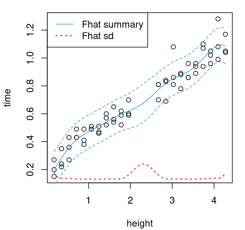

FIGURE 8.2: GP fit to field data; predictive standard deviation is along the bottom in dashed-red.

For my taste, this predictive surface is too wiggly. Surely these data ought to follow a monotonic, if noisy relationship. Uncertainty is too high in the gap, compared against what I would expect intuitively. Maybe some extra modeling could be useful after all. Perhaps coupling with known physics can mitigate those unsightly effects.

What does “Physics 101” say? Time \(t\) to drop a distance \(h\) for gravity \(g\) follows

\[ t = \sqrt{2h/g}. \]

Somewhat realistically, we don’t know the value of \(g\) for the location where the balls were dropped. So gravity is our calibration parameter; our \(u\). Of course there are other unknowns, like air resistance – which will interact deferentially with height/terminal velocity. In other words that mathematical model is biased, and thus there’s scope to improve upon it through hybridization, by coupling with field data. So field data hold the potential to help the computer model as much as the other way around.

At the same time, \(g\) could not just be determined by acceleration due to gravity. At least not with the field data in hand. With more things slowing the ball down than speeding it up, \(g\) will almost certainly be forced into a role of compromise. To account for air resistance, say, estimated \(g\) will probably be shifted downward from its true value. This setup lacks a degree of identifiability no matter how we perform statistical inference. But that doesn’t mean the enterprise isn’t worthwhile.

Consider the following computer implementation of our mathematical model, simultaneously mapping natural inputs \((h,g)\) to coded ones \((x,u)\) in \([0,1]^2\).

timedrop <- function(x, u, hr, gr) 
 {
  g <- diff(gr)*u + gr[1]
  h <- diff(hr)*x + hr[1]
  return(sqrt(2*h/g))
 }

Two-vector hr is derived from the field data range, and was defined above for the purpose of generating a predictive grid of heights. The range for gravity specified below restricts our study to \([6,14]\), equivalently defining a (uniform) prior \(p(u)\) in what follows.

gr <- c(6, 14)

Suppose we’re prepared to run timedrop at \(n_M = 21\) input locations, commensurate in size to the number of unique inputs in the field data experiment, but in two dimensions. R code below constructs a maximin LHS (§4.3) in 2d and performs computer model simulations at those locations.

library(lhs) 
XU <- maximinLHS(21, 2)  
yM <- timedrop(XU[,1], XU[,2], hr, gr)

Now let’s train a GP on those realizations, fixing the nugget to a small jitter value to acknowledge the deterministic nature of timedrop simulations.

yMhat <- newGPsep(XU, yM, d=0.1, g=1e-7, dK=TRUE)
mle <- mleGPsep(yMhat, tmin=eps, tmax=10)

Recall that mleGPsep modifies yMhat with updated mle values as a side effect. Next, extract surrogate predictive mean evaluations over a grid of heights, for a span of six equally-spaced potential \(u\)-values.

us <- seq(0, 1, length=6)
XX <- expand.grid(hs, us)
pm <- predGPsep(yMhat, XX, lite=TRUE)

Figure 8.3 offers a visual of those surfaces, with separate curves for each \(u\)-value.

plot(ball)
matlines(heights, matrix(pm$m, ncol=length(us)))

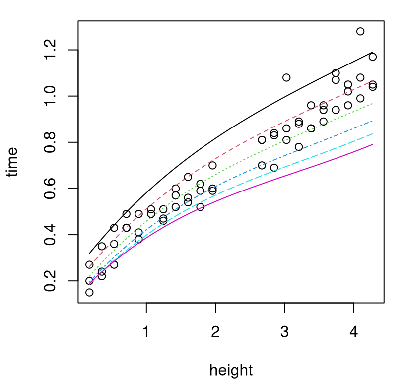
FIGURE 8.3: Computer model surrogates for several settings of calibration parameter \(u\).

Aesthetically, the curves and data in that plot are largely in agreement. Some \(u\)-values generate curves that are better fits than others, yet none are perfect. All exhibit bias. To my eye, the best one is the green-dotted curve in the middle, but it’s clearly biased low for balls dropped from greater heights. When calibrating, it makes sense to account for that bias. When predicting with the computer model, it makes sense to correct for it.

A modularized apparatus calibrates \(u\) via fits for bias. Settings of \(u\) which make residual between surrogate predictions and field data observations “easier” to model are preferred. There are many options for assessing goodness of fit, and throughout this text we’ve preferred maximizing the likelihood, so that’s where we shall start here. The function bhat.fit coded below takes field data (X, yF) and computer model surrogate predictions (e.g., predictive means from a GP) Ym. It also takes prior/initializing specifications for lengthscales (da) and nugget (ga), about which further discussion is provided below.

bhat.fit <- function(X, yF, Ym, da, ga, clean=TRUE)
 {
  bhat <- newGPsep(X, yF - Ym, d=da$start, g=ga$start, dK=TRUE)
  if(ga$mle) cmle <- mleGPsep(bhat, param="both", tmin=c(da$min, ga$min),
    tmax=c(da$max, ga$max), ab=c(da$ab, ga$ab))
  else cmle <- mleGPsep(bhat, tmin=da$min, tmax=da$max, ab=da$ab)
  cmle$nll <- - llikGPsep(bhat, dab=da$ab, gab=ga$ab)
  if(clean) deleteGPsep(bhat)
  else { cmle$gp <- bhat; cmle$gptype <- "sep" }        
  return(cmle)
 }

As you can see, the function initializes and fits a GP to the discrepancy between field data and surrogate (yF - Ym at X) and returns the value of the minimizing negative log likelihood so obtained. As a mathematical abstraction, \(\hat{b}\) is measuring goodness-of-fit for bias no matter how Ym are obtained. Below we shall take Ym \(\equiv\hat{y}^M(X_{n_F}, u)\), and treat \(\hat{b}\) as a merit function for choices of \(u\). Optionally, bhat.fit returns a reference to the fitted GP, although by default this step is skipped (clean=TRUE), causing the object to be freed instead. When searching for \(\hat{u}\) through \(\hat{b}\), we don’t need to save every GP fit en-route, but we will need the last one at the end in order to tap fitted models for prediction. Finally, observe that bhat.fit combines \(\hat{b}\) and \(\hat{\sigma}_\varepsilon^2\) fits via inference for a nugget.

Next create an objective to optimize, over coded gravity \(u\)-values, to find the best setting \(\hat{u}\) estimating unknown \(u^\star\). The calib function below takes argument u in the first position, which is helpful when optimizing with optim, and yMhat in the fourth position. The idea is to provide fit=bhat.fit from above, so that GPs are fit to residuals, where arguments da and ga have been assigned as defaults in advance, as illustrated momentarily. Setting things up in this way, rather than passing da and ga and then calling bhat.fit allows bhat.fit to be swapped out later for another model/fit, if desired, without altering calib. Later in §8.1.4 I shall utilize this feature when presenting a “nobias” alternative.

calib <- function(u, XF, yF, yMhat, fit, clean=TRUE)
 {
  XFu <- cbind(XF, matrix(rep(u, nrow(XF)), ncol=length(u), byrow=TRUE))
  Ym <- predGPsep(yMhat, XFu, lite=TRUE)$mean
  cmle <- fit(XF, yF, Ym, clean=clean)
  return(cmle)
 }

Argument yMhat should be a fitted GP surrogate for computer model runs \((X_{n_M}, Y_{n_M})\). Field data locations X are combined with an extra column of u values and fed into predGPsep to get surrogate means Ym, which are then fed in to fit=bhat.fit.

Rather than shoving calib right into optim, which is exactly what we shall do momentarily, consider first evaluating on a \(u\)-grid to aid visualization. After all, optimizing a deterministic function in 1d is easy with the eyeball norm. The R chunk below sets up such a grid and codes height inputs into \([0,1]\).

u <- seq(0, 1, length=100)
XF <- as.matrix((ball$height - hr[1])/diff(hr))

Before setting this running, arguments da and ga must be specified. Default priors for lengthscales and nuggets may be calculated through darg and garg functions provided with laGP. Observe how these are set up to occupy default values of bhat.fit arguments (i.e., formals).

formals(bhat.fit)$da <- darg(d=list(mle=TRUE), X=XF)
formals(bhat.fit)$ga <- garg(g=list(mle=TRUE), y=ball$time)

Although darg and garg have been used previously to set search ranges and starting values, we’ve not yet discussed their full prior-generating capacity. This is as good a time as any. Respectively, darg and garg offer light regularization through the distribution of pairwise distances in X, and marginal variances in y. In detail, darg calculates default lengthscale search ranges and initializing values from the empirical range of (nonzero) squared Euclidean distances between rows of X, and their 10% quantile, respectively. Gamma prior hyperparameters are chosen to have shape \(a = 3/2\) and rate \(b\) derived by the incomplete Gamma inverse function (DiDonato and Morris Jr 1986) to put 95% of the cumulative Gamma distribution below the maximum such distance observed. The garg routine is similar except that it works with (y - mean(y))^2 instead of pairwise X distances. Another difference is that the starting value is chosen as the 2.5% quantile. Keen readers will note that garg is more squarely targeting priors on \(\sigma_\varepsilon^2 \equiv \tau^2 g\). If knowledge of \(\tau^2\) is available a priori of fitting \(\hat{\tau}^2 \mid g\), then some minor adjustments could help fine-tune priors for \(g\).

Ok, now evaluating on the grid …

unll <- rep(NA, length(u))
for(i in 1:length(u)) 
  unll[i] <- calib(u[i], XF, ball$time, yMhat, bhat.fit)$nll

Before plotting that surface, the code below implements the more hands-off optimize solution, which we can add to the visualization.

obj <- function(x, XF, yF, yMhat, fit) calib(x, XF, yF, yMhat, fit)$nll
soln <- optimize(obj, lower=0, upper=1, XF=XF, yF=ball$time, 
  yMhat=yMhat, fit=bhat.fit)
uhat <- soln$minimum

Figure 8.4 shows that surface and its numerical optimum, our calibrated setting \(\hat{u} \equiv\) uhat.

plot(u, unll, type="l", xlab="u", ylab="negative log likelihood")
abline(v=uhat, col=2, lty=2)
legend("top", "uhat", lty=2, col=2)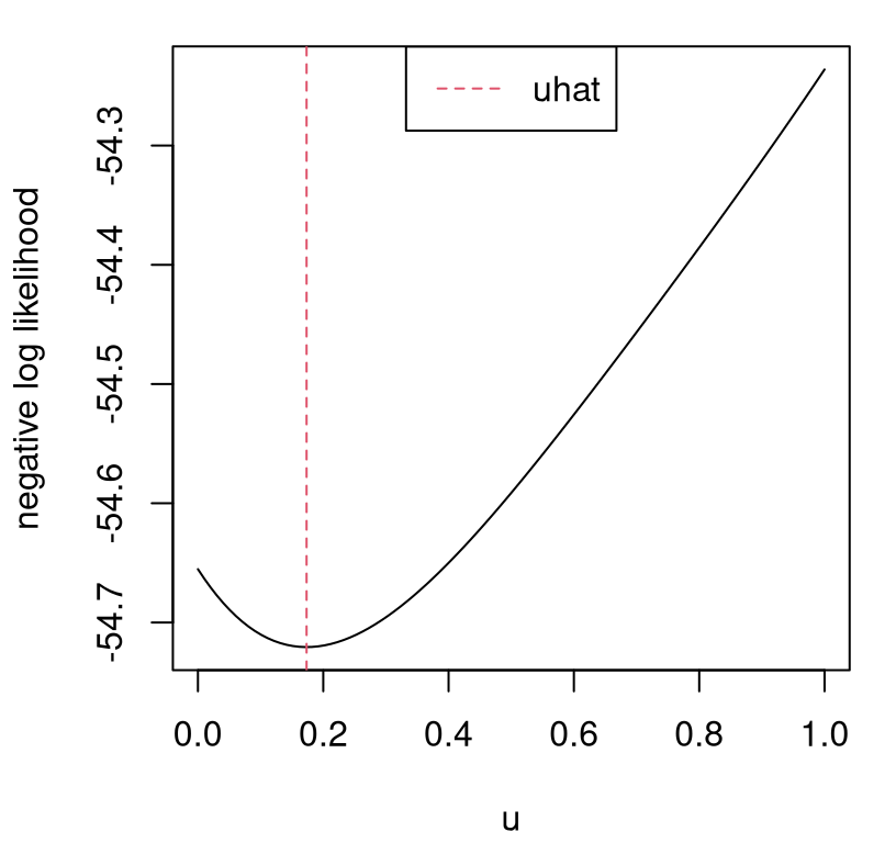

FIGURE 8.4: Negative log likelihood surface for \(u\) and its calibrated value \(\hat{u}\).

Converting back to natural units for the calibration parameter, we can see that our estimate is too low given what we know about acceleration due to gravity on Earth.

ghat <- uhat*diff(gr) + gr[1]
ghat

## [1] 7.387

In fact it’s about 1/3 lower than it should be. Recall that we’re asking gravity to do double-duty. Wiffle balls are exceptionally buoyant compared to other balls, being riddled with holes that trap air. Our mathematical model acknowledges no air resistance. Ideally, such unknowns would be swept entirely into an estimate of bias \(\hat{b}\), however no aspect of the calibration apparatus (whether KOH or modularized) precludes compensation by \(\hat{u}\) instead. Consequently our \(\hat{g}\) above, via \(\hat{u}\), loses some of its physical interpretation. Typically \(\hat{b}\) and \(\hat{u}\) work together to compensate for an imperfect mathematical model and surrogate, challenging identifiability. Further discussion shall have to wait until we get a chance to inspect \(\hat{b}\) in our example below. First, it makes sense to pause that example momentarily to codify the procedure mathematically and algorithmically.

8.1.3 Calibration as optimization

We optimized something (that’s what optim was doing); it ought to be possible, and possibly helpful, to back out a formal criterion and discuss its properties. It all flows from the surrogate \(\hat{y}^M\) and a twist on some notation introduced in §8.1.1, specifically Eqs. (8.1)–(8.2). Let \(\hat{Y}_{n_F}^{M|u} = \hat{y}^M(X_{n_F}, u)\) denote a vector of \(n_F\) emulated output \(y\)-values at inputs \(X_{n_F}\) obtained under a setting \(u\) of the calibration parameter(s). Then, let the computer model surrogate residual \(Y_{n_F}^{b|u} = Y_{n_F} - \hat{Y}_{n_F}^{M|u}\) denote the \(n_F\)-vector of fitted discrepancies. Given these quantities, the quality of a particular \(u\) may be measured by the implied joint probability of observing \(Y_{n_F}\) at inputs \(X_{n_F}\), under our model \(b(\cdot)\) for discrepancies \(Y_{n_F}^{b|u}\).

A GP prior on \(b(\cdot)\) implies that \(\hat{Y}_{n_F}^{b|u} \sim \mathcal{N}(0, \Sigma_n)\), where \(\Sigma_n\) is specified through scaled inverse exponentiated squared Euclidean distances between inputs \(X_{n_F}\), and thus fully specifies that joint probability. The best-fitting GP regression \(\hat{b}(\cdot)\) trained on data \(D_{n_F}^b(u) = (X_{n_F}, \hat{Y}_{n_F}^{b|u})\), viewed as a function of \(u\), defines a likelihood for \(u\). Values of \(u\) which lead to higher such MVN likelihood, i.e., higher probability of observing \(Y_{n_F}\) through those discrepancies, are preferred. So in symbols we have the following mathematical program:

\[\begin{equation} \hat{u} = \mathrm{arg}\max_u \left\{ p(u) \left[ \max_{\theta_b} p_b(\theta_b \mid D^{b}_{n_F}(u))\right] \right\}. \tag{8.4} \end{equation}\]

Recall that \(p(u)\) is a (possibly uniform) prior for \(u\), and \(p_b(\theta_b \mid \cdots)\) denotes a marginal likelihood implied by a GP prior for \(b(\cdot)\), having hyperparameters \(\theta_b\) including scale, lengthscales and nugget. Algorithm 8.2 provides some of the details in pseudocode, with calculations commencing in log space as usual.

Algorithm 8.2: Modularized KOH Calibration by Optimization

Assume computer model simulations \(y^M(\cdot, \cdot)\) are deterministic, and field data are noisy as \(Y^F(\cdot) = y^M(\cdot, u^\star) + b(\cdot) + \varepsilon\), where \(\varepsilon \sim \mathcal{N}(0, \sigma_\varepsilon^2)\). GP priors are not assumed, however examples are given for that canonical choice.

Require prior density \(p(u)\), computer model observations \(Y_{n_M}\) at inputs \((X_{n_M}, U_{n_M})\), field data observations \(Y_{n_F}\) at configurations \(X_{n_F}\), and an initial value \(u^{(0)}\).

Then

1. Fit \(\hat{y}^M(\cdot, \cdot)\) to data \((X_{n_M}, Y_{n_M})\),
   • e.g., by GP and estimated hyperparameters \(\hat{\theta}\) including scale and lengthscales, with mleGPsep(..., param="d").
2. Build an objective to put into an optimizer for calibration parameter \(u\), obj(u), defined as follows:
   1. Obtain surrogate predictive mean values \(\hat{Y}_{n_F}^{M|u} = \mu(X_{n_F}, u)\) from \(\hat{y}^M(\cdot, u)\), e.g., using predGPsep(...)$mean.
   2. Calculate residuals between surrogate predictions and field data locations: \(Y_{n_F}^{b|u} = Y_{n_F} - \hat{Y}_{n_F}^{M|u}\).
   3. Fit \(\hat{b}(\cdot)\) to residual data \((X_{n_F}, Y_{n_F}^{b|u})\),
      • e.g., by GP and estimated hyperparameters \(\hat{\theta}_b\) including scale, lengthscale(s) and nugget with mleGPsep(..., param="both").
   4. Provide as scalar output obj(u) the sum of log prior \(\log p(u)\) plus the maximizing log likelihood value under hyperparameters \(\hat{\theta}_b\),
      • e.g., with llikGPsep(...).
3. Solve \(\hat{u} = \mathrm{argmin}_u -\) obj\((u)\), represented mathematically by Eq. (8.4), with library-based numerical methods,
   • e.g., using optim with method="Nelder-Mead", or method="L-BFGS-B" if \(p(u)\) has support in a hyperrectangle.
4. Rebuild \(\hat{b}\) like in Step 2c above, using \(\hat{u}\).

Return \(\hat{u}\), \(\hat{y}^M(\cdot, \cdot)\), and \(\hat{b}(\cdot)\) so that predictive calculations may be made at new field data locations \(\mathcal{X}\) as \(\hat{y}^M(\mathcal{X}, \hat{u}) + \hat{b}(\mathcal{X})\).

In contrast to “full KOH” in Algorithm 8.1, notice that estimating hyperparameters \(\hat{\theta}\) and \(\hat{\theta}_b\) plays a fundamental role in the inferential process for \(\hat{u}\) and \(\hat{b}\). The algorithm does not presume these to be known at the outset. Accordingly, the outcome of this modularized maximization could be used to set KOH hyperparameters, if desired. Observe in Step 2c that scale (\(\hat{\tau}^2\)) and nugget (\(\hat{g}\)) coordinates of \(\hat{\theta}_b\) are being used implicitly to estimate the field data noise variance as \(\hat{\sigma}_\varepsilon^2 = \hat{\tau}^2 \hat{g}\). In the case where returned predictors \(\hat{y}^M(\mathcal{X}, \hat{u})\) and \(\hat{b}(\mathcal{X})\) are both (approximately) MVN, as they would be under a GP prior, the distribution of their sum would also be MVN because they’re modeled as conditionally independent given \(\hat{u}\). Finally, Step 3 calls for library-based numerical optimization.

One caveat here is that nested optim calls with identical method specifications, as might happen when choosing method="L-BFGS-B" for optimizing over \(u\) and laGP-based methods for calculating MLE hyperparameters for \(\hat{b}(\cdot)\), cause R to crash. A robust but antique BFGS implementation using C static variables confuses the two optimizations and leads to invalid memory access, bringing the whole session down. A simple fix is to use the optim default of method="Nelder-Mead" for \(u\)-optimization instead, perhaps after suitably modifying the objective to check any bound constraints required by \(p(u)\).

It’s worth emphasizing that calibration parameter \(\hat{u}\) is not chosen to minimize bias, but rather is chosen jointly with \(\hat{b}\) to obtain the best correction for that bias, e.g., under a GP prior. The optimization/algorithm above makes this transparent, whereas in Algorithm 8.1 such nuances – which also apply – are somewhat obscured by Metropolis–Hastings details. In fact, it may be that estimates \((\hat{b},\hat{u})\) impart large amplitudes on the bias correction, preferring \(\hat{u}\) that push \(\hat{y}^M(\cdot, \hat{u})\) away from the real process \(y^R(\cdot)\), rather than toward it. For details and further discussion, see Brynjarsdóttir and O’Hagan (2014) and Tuo and Wu (2016).

That’s all to say that we have to be satisfied with \(u\), or gravity \(g\) in our example, being a tuning parameter rather than a primary quantity of interest. If minimal bias is really what we want, then adjustments are needed.⁶ Plumlee (2017) proposes forcing \(b(\cdot)\) to be orthogonal to \(\hat{y}^M\) as a means of obtaining a bias correction that accounts for effects that are missing from computer model simulations, as opposed to those just being “off”. Tuo and Wu (2015) suggest least squares for \(b\) rather than a full GP.⁷ You might ask why we didn’t do this from the very start? Some people do. Both suggestions sacrifice prediction for enhanced interpretation, but unfortunately don’t guarantee identifiability of \(\hat{u}\) except under regularity conditions that are hard to verify/justify in practice. Although there are very good reasons to diverge from the ordinary KOH, in particular to entertain more restrictive models for bias correction, the original GP formulation will be hard to dethrone from its canonical position because it provides accurate predictions for \(Y^F(\cdot)\) out of sample.

The KOH calibration apparatus, and its modularized variation, couples two highly flexible yet well-regularized nonparametric GP models, linked by calibration parameter \(u\). That flexibility is most potent when coping with a data-generating mechanism that may not be faithful to modeling assumptions. (It’s easy to forget that all real data are met with misspecified models in practice.) Authors looking for higher fidelity GP modeling have deliberately deployed similar tactics outside of the calibration setting. Ba and Joseph (2012) coupled two GPs to deal with heteroskedasticity, a form of variance nonstationarity. Bornn, Shaddick, and Zidek (2012) introduced a latent input dimension, just like \(u\), to gain mean-field nonstationarity; L. Johnson et al. (2018) used a similar trick to select between a small number of mean–variance regimes in a real-time disease forecasting framework. Surprisingly, KOH nests both “tricks”, yet precedes them by more than a decade. None cite KOH as inspiration.

Back to the example: bias-corrected prediction

It’s time to return to our ball drop example. Fitted \(\hat{u}\) in hand, we must revisit some of the calculations involved in optimization to back out \(\hat{b}\). Repeated calls to calib created gpi references which, if not immediately destroyed, could have represented a massive memory leak. Providing clean=FALSE to bhat prevents that memory from being recycled, and augments the output object to contain a reference thereto.

bhat <- calib(uhat, XF, ball$time, yMhat, bhat.fit, clean=FALSE)

To visualize that discrepancy, code below gathers predictions over our height grid. Since the fitted GP captures both bias correction \(\hat{b}\) and field data noise \(\hat{\sigma}^2_\varepsilon\), nonug=TRUE is provided to get uncertainty in \(\hat{b}\) only.

pb <- predGPsep(bhat$gp, as.matrix(hs), nonug=TRUE)
sb <- sqrt(diag(pb$Sigma))
q1b <- qnorm(0.95, pb$mean, sb)
q2b <- qnorm(0.05, pb$mean, sb)

Figure 8.5 shows that \(\hat{b}(\cdot)\) surface with means and quantiles extracted above.

plot(heights, pb$mean, type="l", xlab="height", ylab="time bias", 
  ylim=range(c(q1b, q2b)), col=3)
lines(heights, q1b, col=3, lty=2)
lines(heights, q2b, col=3, lty=2)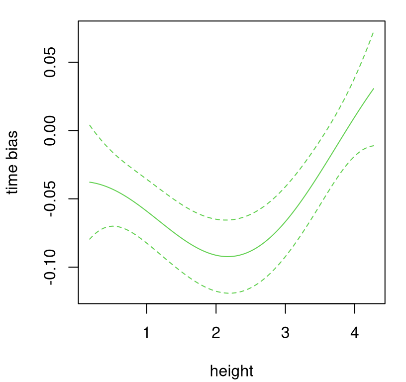 

FIGURE 8.5: Estimated bias correction for the ball drop example.

Observe how bias correction is predominantly negative, or downward, being most extreme for middle heights. Lowest and highest heights require almost no correction, statistically speaking. To combine bias with computer model surrogate, code below obtains predictive equations for \(\hat{y}^M(\cdot)\) on the same height grid, paired with \(\hat{u}\). Quantiles are saved to display the usual three-line summary.

pm <- predGPsep(yMhat, cbind(hs, uhat))
q1m <- qnorm(0.95, pm$mean, sqrt(diag(pm$Sigma)))
q2m <- qnorm(0.05, pm$mean, sqrt(diag(pm$Sigma)))

Means and covariances from \(\hat{y}^M\) and \(\hat{b}\) may be combined additively, leveraging conditional independence.

m <- pm$mean + pb$mean
Sigma.Rhat <- pm$Sigma + pb$Sigma - diag(eps, length(m))

Both GP predictors, representing \(\hat{y}^M\) and \(\hat{b}\) respectively, have covariances augmented with eps jitter along the diagonal in lieu of a fitted nugget to ensure numerical positive definiteness. Adding two of them together results in 2*eps along the diagonal, which is large enough to impart visual jitter on draws from that distribution, calculated momentarily in R below. To compensate, one of those eps augmentations is taken back off. Sample paths so obtained represent approximations to the real process \(R\); they’re realizations from a \(\hat{y}^R(\cdot)\).

library(mvtnorm)
yR <- rmvnorm(30, m, Sigma.Rhat)

In order to accommodate two views into the uncertainty in the reconstructed real process, a second set of predictive equations is calculated for \(\hat{b} + \hat{\sigma}_\varepsilon^2\) as well, yielding \(\hat{Y}^F\). This is essentially the same predict command on bhat$gp as above, but without nonug=TRUE. Quantiles are saved for the three-line predictive summary.

pbs2 <- predGPsep(bhat$gp, as.matrix(hs))
s <- sqrt(diag(pm$Sigma + pbs2$Sigma))
q1 <- qnorm(0.95, m, s)
q2 <- qnorm(0.05, m, s)
deleteGPsep(bhat$gp)

Figure 8.6 provides these two views, with computer model fit \(\hat{y}^M\) and samples from \(\hat{y}^R\) on the left, and a summary of \(\hat{Y}^F\) on the right.

par(mfrow=c(1,2))
plot(ball)
lines(heights, pm$mean)
lines(heights, q1m, lty=2)
lines(heights, q2m, lty=2)
matlines(heights, t(yR), col="gray", lty=1)
legend("bottomright", c("Mhat summary", "Mhat + bhat draws"), 
  lty=c(1,1), col=c("black", "gray"))
plot(ball)
lines(heights, pm$mean + pb$mean, col=4)
lines(heights, q1, col=4, lty=2)
lines(heights, q2, col=4, lty=2)
legend("topleft", "yMhat + bhat + s2", bty="n")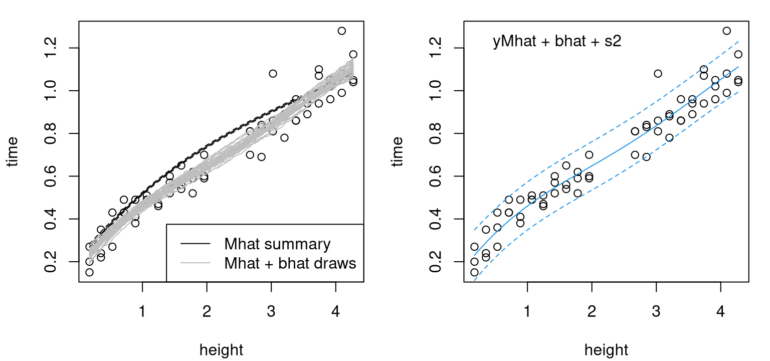

FIGURE 8.6: Modularized KOH predictive distribution via draws (left) and summaries (right).

In the left panel, notice how the surrogate with our estimated calibration parameter, \(\hat{y}^M(\cdot, \hat{u})\), way over-predicts. Recall that KOH considers likelihood of the residual process under a GP; it doesn’t target minimal bias. Also observe how uncertainty on \(\hat{y}^M(\cdot, \hat{u})\) is very low across the heights entertained. Black-dashed quantile lines nearly cover the solid mean line. Samples from the joint predictive distribution of \(\hat{y}^R\) in gray are tight. That distribution could similarly have been represented as a three-line summary, with means and quantiles. However, I chose to show sample paths instead in order to remind readers of the value of full covariance structures. Some lines are more “bendy” than others. But all are much smoother than the mean line from Figure 8.2, back at the very start of this example, where field data were fit directly, without the aid of a computer model. The resulting predictive surface for field measurements, shown in the right panel, is much smoother than the surface from that first fit. Error-bars remain narrow even across the gap in training data. KOH predictors borrow strength from computer model surrogates in regions absent of field data.

That the computer model surrogate is monotonically increasing inside the range of heights under study, but predictive distributions for real and field processes are not, is interesting to note. We may be observing an inflection point in the process where dominant dynamics change. If I were to guess, I’d say that wiffle balls don’t reach their terminal velocity until they’re dropped from heights above 2.5 meters or so, at which point turbulent air and other factors dominate dynamics. Perhaps it takes a few meters for air to freely circulate within the ball, through its Swiss cheese-like holes, ultimately causing the ball to slow down a bit. This aspect may be interesting to investigate further through a more elaborate mathematical model and computer code.

8.1.4 Removing bias

An alternative explanation is that we’re doing a bad job of estimating \(\hat{u}\) and \(\hat{b}\). Perhaps we’d be better off with a simpler apparatus: one without bias correction, say. To entertain that notion, riffing on themes first described by Cox, Park, and Singer (2001), the code below implements an alternative to bhat.fit.

se2.fit <- function(X, yF, Ym, clean=TRUE)
 {
  gp <- newGP(X, yF - Ym, d=0, g=0)
  cmle <- list(nll=-llikGP(gp))
  if(clean) deleteGP(gp)
  else { cmle$gp <- gp; cmle$gptype <- "iso" }
  return(cmle)
 }

Providing d=0 and g=0 tells newGP not to fit a covariance structure, but instead calculate quantities depicting a zero-mean, iid noise, process ignoring inputs X. No mleGP commands are required since scale \(\hat{\tau}^2\) is estimated automatically, in closed form, within newGP. I thought ahead and built calib to accept any discrepancy-fitting function as an argument, even bias-free se2.fit. R code below evaluates calib with fit=se2.fit on our \(u\)-grid from earlier, to help visualize, and then creates an objective for optimization in order to more precisely estimate \(\hat{u}\).

unll.se2 <- rep(NA, length(u))
for(i in 1:length(u)) 
  unll.se2[i] <- calib(u[i], XF, ball$time, yMhat, fit=se2.fit)$nll
obj.nobias <- function(x, XF, yF, yMhat, fit) 
  calib(x, XF, yF, yMhat, fit)$nll
soln <- optimize(obj.nobias, lower=0, upper=1, XF=XF, yF=ball$time, 
  yMhat=yMhat, fit=se2.fit)
uhat.nobias <- soln$minimum

Figure 8.7 shows the resulting surface and estimate of \(\hat{u}\), with old \(\hat{u}\) (under GP bias correction) added on for reference.

plot(u, unll.se2, type="l", xlab="u", ylab="negative log likelihood")
abline(v=uhat, col=2, lty=2)
abline(v=uhat.nobias, col=3, lty=3)
legend("bottomright", c("uhat", "uhat nobias"), lty=2:3, col=2:3)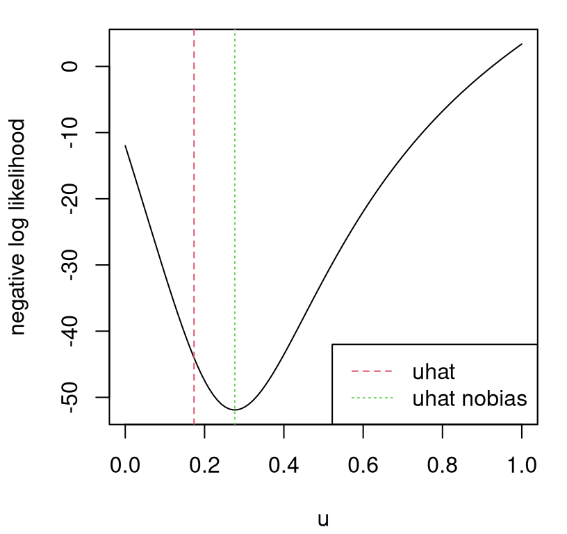

FIGURE 8.7: Likelihood surface for \(u\) and \(\hat{u}\) under the nobias alternative.

Our new estimate of \(\hat{u}\) is higher than before, but after converting back to natural units (of gravity) we see that it’s still probably too low; perhaps estimates are still compensating for air resistance.

ghat.nobias <- uhat.nobias*diff(gr) + gr[1]
ghat.nobias

## [1] 8.21

Visualizing the resulting predictive surface for \(\hat{Y}^F\) requires running back through calib with clean=FALSE, and then combining computer model predictions \(\hat{y}^M(\cdot, \hat{u})\) with noise.

cmle.nobias <- calib(uhat.nobias, XF, ball$time, yMhat, 
  se2.fit, clean=FALSE)
se2.p <- predGP(cmle.nobias$gp, as.matrix(hs), lite=TRUE)
pm.nobias <- predGPsep(yMhat, cbind(hs, uhat.nobias), lite=TRUE)
q1nob <- qnorm(0.05, pm.nobias$mean, sqrt(pm.nobias$s2 + se2.p$s2))
q2nob <- qnorm(0.95, pm.nobias$mean, sqrt(pm.nobias$s2 + se2.p$s2))
deleteGP(cmle.nobias$gp)

Figure 8.8 provides the usual three-line summary.

plot(ball)
lines(heights, pm.nobias$mean, col=4)
lines(heights, q1nob, col=4, lty=2)
lines(heights, q2nob, col=4, lty=2)
legend("topleft", c("yMhat + se2"), col=4, lty=1, lwd=2)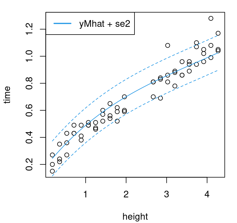

FIGURE 8.8: Nobias predictive surface; compare with Figure 8.6.

Compared to our initial bias corrected version, the curves in the figure are more monotonic but they also perhaps systematically under-predict for all but the lowest drops. So we have two competing fits. How, besides aesthetically, can one choose between them? Answer: out-of-sample validation, e.g., cross validation (CV). The code chunk below collects fitting and prediction code from above into a stand-alone function that can be called repeatedly, in a leave-one-out fashion. The first argument takes a set of predictive locations, XX, whereas the rest accept field data, computer model fit (i.e., pre-fit gpi reference), and discrepancy fitting method. Like calib, implementation here is designed to be somewhat modular to this final choice, say using fit=bhat.fit or fit=se2.fit.

calib.pred <- function(XX, XF, yF, yMhat, fit)
 {
  soln <- optimize(obj, lower=0, upper=1, XF=XF, yF=yF, 
    yMhat=yMhat, fit=fit)
  bhat <- calib(soln$minimum, XF, yF, yMhat, fit, clean=FALSE)
  if(bhat$gptype == "sep") pb <- predGPsep(bhat$gp, XX, lite=TRUE)
  else pb <- predGP(bhat$gp, XX, lite=TRUE)
  pm <- predGPsep(yMhat, cbind(XX, soln$minimum), lite=TRUE)
  m <- pm$mean + pb$mean
  s2 <- pm$s2 + pb$s2 
  q1 <- qnorm(0.95, m, sqrt(s2))
  q2 <- qnorm(0.05, m, sqrt(s2))
  if(bhat$gptype == "sep") deleteGPsep(bhat$gp)
  else deleteGP(bhat$gp)
  return(list(mean=m, s2=s2, q1=q1, q2=q2, uhat=soln$minimum))
 }

Next comes a leave-one-out CV (LOO-CV) loop over \(n_F = 63\) field data points, alternately holding out each as a testing set, training on the others, and then predicting. Note that throughout we are conditioning on the same computer model surrogate yMhat, fit to the full computer experiment. CV is over field data only. Each iteration first considers the usual bias correcting modularized KOH setup, and then a simpler nobias alternative.

uhats <- q1 <- q2 <- m <- s2 <- rep(NA, nrow(XF))
uhatsnb <- q1nb <- q2nb <- mnb <- s2nb <- uhats
for(i in 1:nrow(XF)) {
  train <- XF[-i,,drop=FALSE]
  test <- XF[i,,drop=FALSE]
  cp <- calib.pred(test, train, ball$time[-i], yMhat, bhat.fit)
  m[i] <- cp$mean
  s2[i] <- cp$s2 
  q1[i] <- cp$q1
  q2[i] <- cp$q2 
  uhats[i] <- cp$uhat
  cpnb <- calib.pred(test, train, ball$time[-i], yMhat, se2.fit)
  mnb[i] <- cpnb$mean
  s2nb[i] <- cpnb$s2
  q1nb[i] <- cpnb$q1
  q2nb[i] <- cpnb$q2
  uhatsnb[i] <- cpnb$uhat
}

Summary statistics, such as field data predictive quantities at \(x_i\) along with \(\hat{u}_i\), for \(i=1,\dots,n_F\), have been saved for subsequent inspection. For example, Table 8.2 shows what \(\hat{u}\)-values we get in the bias correcting case, including values mapped back to natural units of gravity.

kable(rbind(u=summary(uhats), g=summary(uhats)*diff(gr) + gr[1]),
  caption="Jackknife distribution for $\\hat{u}$.")

TABLE 8.1: Jackknife distribution for \(\hat{u}\).

	Min.	1st Qu.	Median	Mean	3rd Qu.	Max.
u	0.1154	0.1652	0.1728	0.1732	0.1797	0.2486
g	6.9235	7.3219	7.3824	7.3858	7.4373	7.9886

Quite a big range actually. Some are very small indeed. Others are substantially larger, but none nearly as large as the nominal value of \(9.8 m/s^2\) on Earth. That summary is of a so-called jackknife sampling distribution, a precursor to the bootstrap which would perhaps represent a more standard alternative to studying the sampling distribution of \(\hat{u}\) in modern times. (That is, beyond the Bayesian option we started the chapter with, and to which we shall return in §8.1.5.) Resampling methods like the bootstrap are simple and sufficient when field data are plentiful.

Table 8.2 summarizes the jackknife distribution for \(\hat{u}\) from the nobias alternative.

kable(rbind(u=summary(uhatsnb), g=summary(uhatsnb)*diff(gr) + gr[1]), 
  caption="Jackknife distribution for nobias $\\hat{u}$.")

TABLE 8.2: Jackknife distribution for nobias \(\hat{u}\).

	Min.	1st Qu.	Median	Mean	3rd Qu.	Max.
u	0.2695	0.274	0.2761	0.2763	0.2772	0.2921
g	8.1562	8.192	8.2090	8.2107	8.2173	8.3371

Although substantially higher than their bias-correcting analog, this distribution is still shifted substantially lower than nominal. In both cases the computer model surrogate is being asked to compensate for dynamics not accounted for by the underlying mathematical model. Since both come up short on that metric – although we never expected either to do particularly well – a comparison on out-of-sample predictive accuracy grounds seems more practical. Figure 8.9 offers visual inspection on those terms. Each prediction is shown as a filled circle, bias-correcting in red (left panel) and nobias in green (right panel), with similarly colored vertical line segments indicating 90% prediction interval(s).

par(mfrow=c(1,2))
plot(ball, main="bias correcting")
points(ball$height, m, col=2, pch=20)
segments(ball$height, q1, ball$height, q2, col=2)
plot(ball, main="nobias")
points(ball$height, mnb, col=3, pch=20)
segments(ball$height, q1nb, ball$height, q2nb, col=3)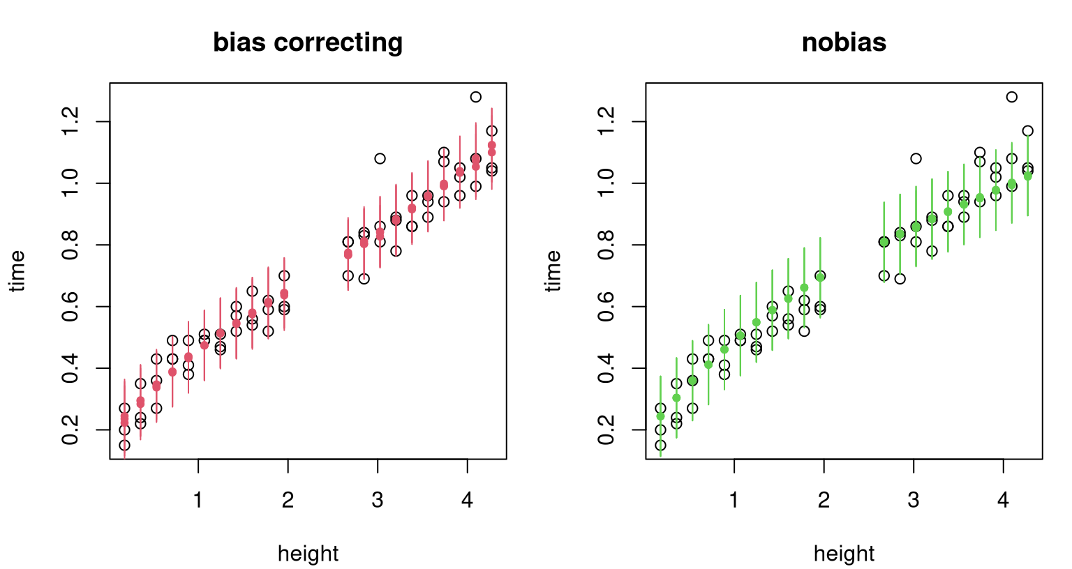

FIGURE 8.9: Leave-one-out CV results in ordinary (left) and nobias (right) alternatives. Filled dots show predictive means; vertical lines indicate 90% intervals.

For my money, the panel on the left looks better: only two dots are left uncovered. On the right I count six dots without a green line going through them at least part way. It’s easy to make such a comparison quantitative with proper scores (Gneiting and Raftery 2007). Eq. (27) from that paper covers pointwise cases: means and variances, without full covariance; i.e., Eq. (5.6) from §5.2.1 forcing diagonal \(\Sigma(\mathcal{X})\).

b <- mean(- (ball$time - m)^2/s2 - log(s2))
nb <- mean(- (ball$time - mnb)^2/s2nb - log(s2nb))
scores <- c(bias=b, nobias=nb)
scores

##   bias nobias 
##  4.187  3.981

Higher scores are better, so correcting for bias wins.

Modularized KOH calibration isn’t perfect, but it’s relatively simple to solve with library methods for GP fitting and for optimization to find \(\hat{u}\). Resulting predictions are accurate owing to flexibility as much as to information quality, provided down the chain of mathematical model, simulation data and field experiment. Although there are many variations, and we briefly discussed a few, the presentation above mainly covers highlights targeting robust implementation. Opportunities for stress-testing are provided by homework exercises both here in §8.3 and (with minor modification to handle big simulation data) on our motivating radiative shock hydrodynamics example (§2.2) in §9.4.

8.1.5 Back to Bayes

As a capstone, and because I said we would, let’s return back to full KOH and think about posterior sampling conditional on GP hyperparameters estimated with the modularized variation above. We shall follow Algorithm 8.1, whose most important calculation is covariance \(\mathbb{V}(u)\). The top-left block of \(\mathbb{V}(u)\) is \(\Sigma_{n_M}\), capturing computer model surrogate covariance on design \([X_{n_M}, U_{n_M}]\). Observe that \(\Sigma_{n_M}\) doesn’t depend upon \(u\). Using \(\hat{\theta}\) stored in mle (and scale \(\hat{\tau}^2\) derived thereupon, in closed form), \(\Sigma_{n_M}\) may be calculated as follows.

library(plgp)
KM <- covar.sep(XU, d=mle$d, g=eps)
tau2M <- drop(t(yM) %*% solve(KM) %*% yM / length(yM))
SigmaM <- tau2M*KM

A portion of bottom-right block of \(\mathbb{V}(u)\), namely \(\Sigma_{n_F}^b\), also doesn’t depend on \(u\). This matrix measures bias covariance between field data locations, conditioned on parameters \(\hat{\theta}_b\), including noise level \(\hat{\sigma}_\varepsilon^2\) via an estimated nugget. Calculations below borrow \(\hat{\theta}_b\) from bhat. Completing the hyperparameter specification with \(\hat{\tau}_b^2\) requires predictions from the computer model, which may be obtained by applying predGPsep on yMhat with \(\hat{u}\) calculated above.

KB <- covar.sep(XF, d=bhat$theta[1], g=bhat$theta[2])
XFuhat <- cbind(XF, 
  matrix(rep(uhat, nrow(XF)), ncol=length(uhat), byrow=TRUE))
Ym <- predGPsep(yMhat, XFuhat, lite=TRUE)$mean
YmYm <- ball$time - Ym
tau2B <- drop(t(YmYm) %*% solve(KB) %*% YmYm / length(YmYm))
SigmaB <- tau2B * KB
deleteGPsep(yMhat)

Remaining components of \(\mathbb{V}(u)\) depend upon \(u\) and must be rebuilt on demand for each newly proposed value of \(u\) as MCMC iterations progress. \(\Sigma_{n_M}(X_{n_F}, u)\) measures covariance between \([X_{n_M}, U_{n_M}]\) and \([X_{n_F}, u^\top]\) under the surrogate. Notation \([X_{n_F}, u^\top]\) is shorthand for a design derived by concatenating \(u\) to each row of field data inputs \(X_{n_F}\). Similarly \(\Sigma_{n_F}(u)\) captures surrogate covariance between \([X_{n_F}, u^\top]\) and itself. Both are calculated by the function coded below, which subsequently completes \(\mathbb{V}(u)\) by combining with \(\Sigma_{n_M}\) and \(\Sigma_{n_F}^b\), e.g., as saved from earlier calculations like those immediately above.

ViVldet <- function(u, XU, XF, SigmaM, tau2M, mle, SigmaB)
 {
  ## build blocks
  XFu <- cbind(XF, u)
  SMXFu <- tau2M * covar.sep(XU, XFu, d=mle$d, g=0)
  SMu <- tau2M * covar.sep(XFu, d=mle$d, g=eps)

  ## build V from blocks
  V <- cbind(SigmaM, SMXFu)
  V <- rbind(V, cbind(t(SMXFu), SMu + SigmaB))

  ## return inverse and determinant
  ## (improvements possible with partitioned inverse equations)
  return(list(inv=solve(V), 
    ldet=as.numeric(determinant(V, log=TRUE)$modulus)))
 }

Observe that ViVldet doesn’t return \(\mathbb{V}(u)\) but rather its inverse and determinant as required by the log likelihood (8.3). Code below implements a function calculating that quantity up to an additive constant.

llik <- function(u, XU, yM, XF, yF, SigmaM, tau2M, mle, SigmaB)
 {
  V <- ViVldet(u, XU, XF, SigmaM, tau2M, mle, SigmaB)
  ll <- - 0.5*V$ldet
  Y <- c(yM, yF)
  ll <- ll - 0.5*drop(t(Y) %*% V$inv %*% Y)
  return(ll)
 }

Although llik takes a multitude of arguments, repeated calls in an MCMC loop would only vary its first argument, u. In order to simplify calls to llik in the Metropolis–Hastings (MH) scheme coming shortly, the code below sets the latter eight arguments as defaults using quantities from/derived for our ball drop experiment. That leaves u as the only unspecified argument in llik, establishing a convenient shorthand.

formals(llik)[2:9] <- list(XU, yM, XF, ball$time, SigmaM, tau2M, 
  mle, SigmaB)

The final ingredient is the prior. One option is uniform over the study area \(g \in [6,14]\), mapping to \(u \in [0,1]\) in coded units. Beta priors, generalizing the uniform, are also popular, often with shape parameters (\(> 1)\) that mildly discourage concentration of posterior on boundaries of the study region. For our example below, I chose a beta prior of this kind but over a somewhat wider space, \(u \in [-0.75, 2]\) which maps to \(g \in [0,22]\). The result is a relatively flat prior over the study region \([6,14]\), emphasizing values nearby \(9.8 m/s^2\) and discouraging pathological/extreme values such as \(g=0\) on the low end, and \(g\) bigger than two-times nominal on the high end.

lprior <- function(u, shape1=1.1, shape2=1.1, lwr=-0.75, upr=2) 
 {
  u <- (u - lwr)/(upr - lwr)
  dbeta(u, shape1, shape2, log=TRUE)
 }

Ok, we’re ready for MCMC. Below, space is allocated for \(10^4\) samples from the posterior. Initial values are specified for the chain using \(\hat{u}\) calculated above.

T <- 10000
lpost <- u <- rep(NA, T)
u[1] <- uhat
lpost[1] <- llik(u[1]) + lprior(u[1])

A for loop implements a random walk Metropolis sampler (see, e.g., Sherlock, Fearnhead, and Roberts 2010) using Gaussian proposals with variance \(0.3^2\) (sd=0.3), tuned to ensure good mixing of the Markov chain. Symmetry in that proposal choice simplifies expressions involved in MH accept–reject calculations since the ratio of proposal densities (\(q\)), or equivalently the difference of their logs, cancel. Since such a scheme can generate innovations outside the study area, a check on the prior is required in order to short circuit handling of proposals which violate support constraints.

for(t in 2:T) {
  
  ## random walk Gaussian proposal
  u[t] <- rnorm(1, mean=u[t - 1], sd=0.3)
  lpu <- lprior(u[t])
  if(is.infinite(lpu)) { ## prior reject
    u[t] <- u[t - 1]
    lpost[t] <- lpost[t - 1]
    next
  }

  ## calculate log posterior
  lpost[t] <- llik(u[t]) + lpu

  ## Metropolis accept-reject calculation
  if(runif(1) > exp(lpost[t] - lpost[t - 1])) { ## MH reject
    u[t] <- u[t - 1]
    lpost[t] <- lpost[t - 1]
  }
 }

Figure 8.10 shows a trace plot of samples obtained from the Markov chain targeting the posterior distribution for \(u\) under KOH. Mixing is visually very good, and by initializing with the MLE the chain reaches stationarity instantaneously.

plot(u, type="l", xlab="MCMC iteration 1:T", ylab="u")

FIGURE 8.10: MCMC trace plot for KOH calibration.

One way to assess MCMC quality, and thereby efficiency of the sampler, is through effective sample size [ESS; Kass et al. (1998)]. Out of a total of \(T = 10^{4}\) sequentially correlated MCMC samples, ESS measures about how many independent samples that’s worth through a measurement of autocorrelation in the chain.

library(coda)
ess <- effectiveSize(u)
ess

##  var1 
## 648.9

In this case, about one in each of 15 samples can be regarded as independent, having “forgotten” the past from which it came. One way to improve upon that may be to adjust proposal variance. For our purposes 649 samples is good enough to summarize the empirical distribution, say with a kernel density.

d <- density(u*diff(gr) + gr[1], from=0, to=22)

Before plotting that density in Figure 8.11, R code below evaluates the prior over a grid in \(u\)-space for comparison. To ease interpretation, the \(x\)-axis in the plot is provided in natural units of gravity.

ugrid <- seq(-0.75, 2, length=1000)
ggrid <- ugrid*diff(gr) + gr[1]
lp <- lprior(ugrid)
plot(d, xlab="g", lwd=2, main="")
lines(ggrid, exp(lp)/30, col="gray")
abline(v=ghat, col=2, lty=2)
legend("topright", c("uhat", "prior", "posterior"), lty=c(2,1,1), 
  col=c("red", "gray", "black"), lwd=c(1,1,1,2), bty="n")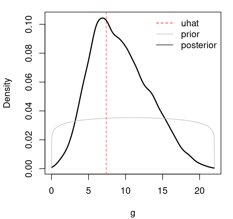

FIGURE 8.11: Comparing posterior, prior and \(\hat{u}\) for KOH calibration.

A takeaway from the figure is that there is, at best, modest information in the likelihood relative to the prior. We have a posterior density whose mass is shifted slightly to the right, away from the likelihood (or posterior under a uniform prior) and toward the prior. As a result, the most probable setting for the unknown gravitational acceleration parameter is substantially lower than the nominal value.

w <- which.max(lpost)
u[w]*diff(gr) + gr[1]

## [1] 7.262

Another way to view this state of affairs is through the lens of bias correction. It would appear that our GP fit to discrepancies between computer model and field data is able to cope with almost any reasonable value of \(u\). Some cause less trouble than others, but on the whole \(u\)-coupled GPs enjoy more than enough flexibility to explain dynamics exhibited by field and simulation data in a variety of ways. Some of those ways entail seemingly contradictory hypotheses through extremely low and high degrees of gravitational force.

Samples from the posterior distribution for \(u\) in hand, and implicitly also for \(b(\cdot)\), the next step is to convert those into samples from the posterior predictive distribution for \(Y^F(x)\), potentially for many \(x \in \mathcal{X}\). Each sample from the posterior, \(u^{(t)}\), can be used to define a conditional predictive distribution for \(Y^F(\mathcal{X}) \mid Y_{n_F}, Y_{n_M}, u^{(t)}\). A homework exercise in §8.3, which we’ve alluded to once before but it bears repeating, asks the curious reader to derive that distribution by first expanding MVN covariance structure \(\mathbb{V}(u^{(t)})\) to include new rows/columns representing the distribution of all three sets of \(Y\)-values jointly, and subsequently applying MVN conditioning identities (5.1). Then, averaging over all \(t=1,\dots,T\) yields an empirical predictive density that marginalizes over uncertainty in the calibration parameter, approximating

\[ p(Y^F(x) \mid Y_{n_F}, Y_{n_M}) = \int_{\mathcal{U}} p(Y^F(x) \mid u, Y_{n_F}, Y_{n_M}) \cdot p(u \mid Y_{n_F}, Y_{n_M}) \; du. \]

Predictive distributions which integrate out all unknowns are a hallmark of Bayesian analysis. Recall that we’ve conditioned upon hyperparameters from the earlier modularized analysis. A fully Bayesian calibration, extending MCMC to hyperparameters for both GPs, can dramatically expand the complexity of the overall scheme. This usually represents overkill, however there are settings where a full accounting of all uncertainties is essential.

Theoretically minded but practically aware

There are many schools of thought on the right way to calibrate and simultaneously quantify uncertainty, but few recipes which are readily deployable out of the box. MATLAB® software called GPMSA is perhaps the first suite of its kind, providing surrogate modeling and computer model calibration capabilities (Gattiker et al. 2016). Two packages on CRAN called CaliCo (Carmassi 2018) and BACCO (Hankin 2013) offer a Bayesian approach similar to the one implemented above, with some of the extensions left here to exercises in §8.3.

One of the great advantages of the Bayesian paradigm is that it exposes model inadequacies by giving ready access to estimation uncertainties. In the KOH case “inadequacy” manifests as extreme flexibility, which is a paradox. Modularization helps because it limits flexibility somewhat through a more constrained prior, allowing only computer model runs to influence surrogate fits. Nevertheless confounding and identifiability are ever-present concerns (Gu and Wang 2018; Gu 2019).

There are many reasons to calibrate, with KOH or otherwise. One is simply predictive; another is to get a sense of how the apparatus could be tuned, or to quantify how much information is in the data (and prior) about promising \(u\) settings. Both are very doable, and worth doing, even in the face of confounding. When causal interpretation is essential, further constraints such as limiting forms of bias correction (Plumlee 2017; Tuo and Wu 2015) can help with posterior identifiability of \(u\), but often at the expense of predictive accuracy.

Fully Bayesian prediction at the field level, \(Y^F(\mathcal{X})\) via ordinary KOH as above and in the homework, is hard to beat. Other, more complicated but also more satisfying examples are offered up as further homework exercises. More ambitious “big simulation” analogs in §9.3.6, as motivated by the radiative shock hydrodynamics example of §2.2, benefit from the thriftier, more modular approach.

8.2 Sensitivity analysis

In any nonparametric regression setting, but especially when two nonparametric regressions are coupled together as in §8.1, it’s important to understand the role inputs play in predicted outputs. When inputs change, how do outputs change? In simple linear regression, estimated slope coefficients \(\hat{\beta}_j\) and their standard errors speak volumes, resulting in \(t\)-tests or \(F\)-tests to ascertain relevance. Or, we may inspect leverage or Cook’s distance to focus on particular input–output pairs. By contrast, the effect of fitted GP hyperparameters and input settings on predictive surfaces is subtle and sometimes counter-intuitive. In a way, that’s what nonparametric means: parameters don’t unilaterally dictate what’s going on. Model fits and predictive equations gain flexibility from data, sometimes with the help of – but equally often in spite of – any estimated tuning or hyperparameters.

Because of the complicated nature by which data affect fit and predictor in nonparametric regression, approaches to decomposing the effects of inputs \(x\) on outputs \(Y\) in that setting are varied. Many methods focus in particular on GP regression, but with no less diversity despite (model) specificity. Oakley and O’Hagan (2004) offer what is perhaps the first complete treatment, although efforts date back to Welch et al. (1992) with revisions from R. Morris et al. (2008).

The approach presented here has many aspects in common with these ideas, and with Marrel et al. (2009), whose analysis tailors first-order Sobol indices (Sobol 1993, 2001) to surrogates derived from GP predictive equations. Yet our presentation will lean more generic. By not focusing expressly on GP equations we can, among other things, accommodate a higher-order analysis under a more unified umbrella. Our approach follows the Saltelli (2002) school of thought in numerical integration: what happens to predictive means and variances when fixing some input coordinates and integrating out others? While illustrations will focus on GP regression, as our preferred surrogate, I won’t leverage GPs in our methodological development. The edited volume by Saltelli, Chan, and Scott (2000) provides an overview of the field. Valuable recent work on smoothing methods (Storlie and Helton 2008; Da Veiga, Wahl, and Gamboa 2009; Storlie et al. 2009) provide a nice overview of nonparametric regression coupled with sensitivity analysis.

8.2.1 Uncertainty distribution

If we’re going to say how sensitive outputs are to changes in inputs, it makes sense to first say what inputs we expect/care about, and how much they themselves may change/vary. Underlying the Saltelli method is a reference distribution for \(x\), sometimes called an uncertainty distribution \(U(x)\). \(U\) can represent uncertainty about future values of \(x\), or the relative amount of research interest in various areas of the input space. In many applications, the uncertainty distribution is simply uniform over a bounded region.

In Bayesian optimization (Chapter 7), \(U\) can be used to express prior information from experimentalists or modelers on where to look for solutions. For example, when there’s a large number of input variables over which an objective function is to be optimized, typically only a small subset will be influential within the confines of their uncertainty distribution. Sensitivity analysis can be used to reduce the volume of the search space of such optimizations (Taddy et al. 2009). Finally, in the case of observational systems such as air-quality or smog levels (§8.2.4), \(U(x)\) may derive from an estimate of the density governing natural occurrence of \(x\) factors, e.g., air pressure, temperature, wind and cloud cover. In such scenarios, sensitivity analysis attempts to resolve natural variability in responses \(Y(x)\).

Although one can adapt the type of sampling described shortly to account for correlated inputs in \(U\) (Saltelli and Tarantola 2002), we treat here the standard and computationally convenient independent specification,

\[ U(x) = \prod_{k=1}^m u_k(x_k), \]

where \(u_k\), for \(k=1,\dots, m\), represent densities assigned to the margins of \(x\). With \(U\) being specified probabilistically, readers may not be surprised to see sampling feature as a principal numerical device for averaging over uncertainties, i.e., over variability in \(U\). Such averages approximate expectations, which are integrals. Latin hypercube sampling (LHS; §4.1) was conceived to reduce variability in exactly that sort of Monte Carlo (MC) approximation to integrals. Accordingly, LHSs with margins \(u_k\) feature heavily in our Saltelli-style calculation of Sobol sensitivity indices.

8.2.2 Main effects

The simplest sensitivity indices are main effects, which deterministically vary one input variable, \(j\), while averaging others over \(U_{-j}\):

\[\begin{equation} \mathrm{me}(x_j) \equiv \mathbb{E}_{U_{-j}} \{y \mid x_j\} = \int\!\!\int_{\mathcal{X}_{-j}} \! y p(y \mid x_1, \dots, x_m) \cdot u_{-j}(x_1, x_{j-1}, x_{j+1}, x_m) \, dx_{-j} dy. \tag{8.5} \end{equation}\]

Above, \(u_{-j} = \prod_{k \ne j} u_k(x_k)\) represents density derived from the joint distribution \(U\) without coordinate \(j\), i.e. \(U_{-j}\) with \(\mathcal{X}_{-j}\) and \(x_{-j}\) defined similarly, and \(p(y \mid x_1, \dots, x_m) \equiv p(Y \mid x) \equiv p(Y(x) = y)\) comes from the surrogate, e.g., a GP predictor.

Algorithmically, calculating main effects proceeds as follows: grid out \(\mathcal{X}\)-space in each coordinate with values \(x_{ji}\), for \(i=1,\dots,G\) say; gather \(\mathrm{me}(x_{ji})\)-values holding the \(j^{\mathrm{th}}\) coordinate fixed at each \(x_{ji}\), in turn, and average over the rest (and \(y\)) in an MC fashion; finally plot all \(\mathrm{me}(x_{ji})\) on a common \(x\)-axis. A pseudocode in Algorithm 8.3 formalizes that sequence of steps with some added numerical detail. The algorithm utilizes samples of size \(N\) in its MC approximations.

Algorithm 8.3: Main Effects

Assume \(m\)-dimensional coded inputs \(x\in [0,1]^m\) and interest in mean main effects \(\mu(x) = \int y p(y\mid x) \; dy\), although \(\mu(x)\) may stand in below for other quantities available from predictive equations.

Require uncertainty distribution \(U\) which may readily be sampled, say with LHS via margins \(u_1,\dots,u_m\); a desired sample size \(N\) controlling accuracy of the MC calculation; surrogate or predictive equations \(p(y \mid x)\), say from a GP, generating \(\mu(x)\) or another quantity of interest; grid \(0 \leq g_1, \dots, g_G \leq 1\) which may be applied separately but identically to each margin of \(x\).

For each coordinate of \(x_j\), as \(j=1,\dots,m\), and each grid element of \(g_i\), as \(i=1,\dots,G\), i.e., a double-“for” loop …

1. Draw \(N\) samples from \(U_{-j}\) and combine with \(g_i\) to create \(N \times m\) predictive matrix \(\mathcal{X}_j\) whose \(j^{\mathrm{th}}\) column has \(N\) copies of \(g_i\) and remaining columns hold the samples.
2. Evaluate the surrogate at \(\mathcal{X}_j\), saving predictive means \(\mu({\mathcal{X}_j})\) in \(N\)-vector \(\hat{y}\),
   • or similarly for another predictive quantity of interest.
3. Average over the \(N\) samples to save approximate \(\mathrm{me}(x_{ji})\) as \(\mathrm{me}_{ji} = \frac{1}{N} \sum_{s=1}^N \hat{y}_{s}\).

End For

Return \(m \times G\) matrix “\(\mathrm{me}\)” or, more commonly, plot each of \(m\) row-vectors \(\mathrm{me}_j\) on a common \(x\)-axis with coordinates \(g_1,\dots,g_G\).

Although Eq. (8.5) and Algorithm 8.3 showcase mean main effects \(\mu(x) = \int y p(y \mid x) \; dy\), any aspect of \(p(y \mid x)\) which may be expressed as an integral can be averaged with respect to \(U\) in this manner. Quantiles are popular, for example, since they may be plotted on the same axes as means.

In situations where sampling from \(U\) is computationally expensive, one may prefer instead to pre-sample a single \(N \times m\) matrix \(\mathcal{U}\) of deviates in lieu of the \(m \times G\) separate \(N \times (m-1)\) samples implied by each iterate of Step 1 within the “for” loop. In that setup, a revised Step 1 would instead de-select the \(j^{\mathrm{th}}\) column to create \(N \times (m-1)\) matrix \(\mathcal{U}_{-j}\), combining with grid entries to create \(\mathcal{X}_j\) in Step 2. Reusing deviates from \(U\) in this manner, where each iterate of the double-“for” loop involves similar \(\mathcal{U}_{-j}\), induces correlation in otherwise independent calculations. That increases MC error which can be mitigated, to a certain extent, with larger \(N\). Whether by pre-sampling, or with the original Step 1, LHS from \(U\) is common as a means of reducing variability for fixed MC sample size \(N\).

Before jumping into an illustration, it’s worth commenting on a common alternative “main effect” that avoids integration over “\(-j\)” input coordinates, instead replacing them with their mean value.

\[ \overline{\mathrm{me}}(x_j) \equiv \mathbb{E}\{y \mid x_j, \bar{x}_{-j}\} \]

This is not the same thing, and it’s not even really a poor man’s approximation. The behavior of responses as a function of typical (average) input values is not the same as average behavior over all input values. But that doesn’t make it wrong or mean it’s not an interesting thing to look at. However most would argue that it provides, at best, a limited view into the effect of inputs on outputs. I tend to agree. Situations where this alternative is, for the most part, adequate correspond to settings where far simpler surrogates (e.g., linear/polynomial) may have been sufficient to begin with. In those situations, the methods of Chapter 3 provide more precise and satisfying results.

To kick the tires a bit, return to the Friedman data (5.12) from §5.2.5 which combines a nice span of nonlinear, linear, and useless effects. The function is pasted below.

fried <- function (n, m=6)
 {
  if(m < 5) stop("must have at least 5 cols")
  X <- randomLHS(n, m)
  Ytrue <- 10*sin(pi*X[,1]*X[,2]) + 20*(X[,3] - 0.5)^2 + 10*X[,4] + 5*X[,5]
  Y <- Ytrue + rnorm(n, 0, 1)
  return(data.frame(X, Y, Ytrue))
 }

To create a dataset for surrogate learning, let’s evaluate fried on a random design of size 250. Then fit a GP surrogate.

data <- fried(250)
gpi <- newGPsep(as.matrix(data[,1:6]), data$Y, d=0.1, 
  g=var(data$Y)/10, dK=TRUE)
mle <- mleGPsep(gpi, param="both", tmin=rep(eps, 2), 
  tmax=c(10, var(data$Y)))

Begin by keeping it simple with uniform \(U(x)\) in \([0,1]^6\). The code chunk below allocates space necessary to calculate MC averages of size \(N=10\)K on a uniform grid of \(G=30\) values in each \(x_j\).

N <- 10000
G <- 30  
m <- q1 <- q2 <- matrix(NA, ncol=6, nrow=G)
grid <- seq(0, 1, length=G)
XX <- matrix(NA, ncol=6, nrow=N)

Then, the double-“for” loop may commence. Below main effects are collected for predictive means, and central 90% predictive quantiles so that we may also inspect error-bars on main effects. Since emphasis here is on the mean, nonug=TRUE is provided when gathering predictive summaries. Although these data are inherently noisy, epistemic uncertainty in main effects should decrease to zero as the number of training data points grows toward infinity (uniformly within a finite study region).

for(j in 1:6) {
  for(i in 1:G) {
    XX[,j] <- grid[i]
    XX[,-j] <- randomLHS(N, 5)
    p <- predGPsep(gpi, XX, lite=TRUE, nonug=TRUE)
    m[i,j] <- mean(p$mean)
    q1[i,j] <- mean(qnorm(0.05, p$mean, sqrt(p$s2)))
    q2[i,j] <- mean(qnorm(0.95, p$mean, sqrt(p$s2)))
  }
}

Figure 8.12 provides a visualization of these mean main effects. Error-bars will be added momentarily, but it’s easier to focus on one thing at a time. There are already six lines in the figure; adding error-bars will make eighteen.

plot(0, xlab="grid", ylab="main effect", xlim=c(0,1), 
  ylim=range(c(q1,q2)), type="n")
for(j in 1:6) lines(grid, m[,j], col=j, lwd=2)
legend("bottomright", paste0("x", 1:6), fill=1:6, horiz=TRUE, cex=0.75)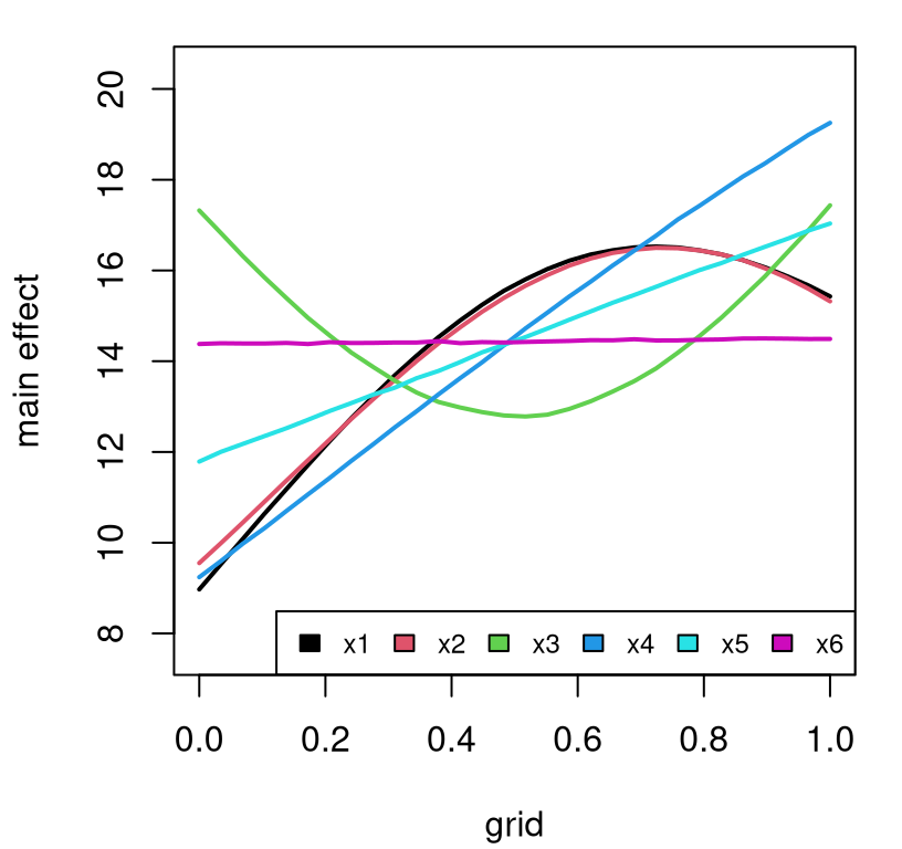

FIGURE 8.12: Mean main effects for Friedman data observed with irrelevant input \(x_6\).

First, note that the scale of the \(y\)-axis isn’t directly meaningful. Apparently, mean responses vary from about ten to twenty. Considering what we know about the Friedman function, the lines in the figure make sense. For example, \(x_1\) and \(x_2\) contribute in a similar, non-linear (perhaps sinusoidal) manner. Since they only interact in a product, their effects are indistinguishable from one another when holding one fixed and averaging over the other. Input \(x_3\) augments with a face-up parabola; \(x_4\) and \(x_5\) factor in linearly. Finally, \(x_6\) is flat. It has no effect on the response when averaging over other inputs.

Figure 8.13 updates with 90% central error-bars. Observe that there’s substantial variability in these main effects. Still, changes in mean main effects across the \(x\)-axis far exceeds the width of the interval(s) for all except input \(x_6\). We have our first indication that \(x_6\) is a useless input.

plot(0, xlab="grid", ylab="main effect", xlim=c(0,1), 
  ylim=range(c(q1,q2)), type="n")
for(j in 1:6) { 
  lines(grid, m[,j], col=j, lwd=2)
  lines(grid, q1[,j], col=j, lty=2)
  lines(grid, q2[,j], col=j, lty=2) 
}
legend("bottomright", paste0("x", 1:6), fill=1:6, horiz=TRUE, cex=0.75)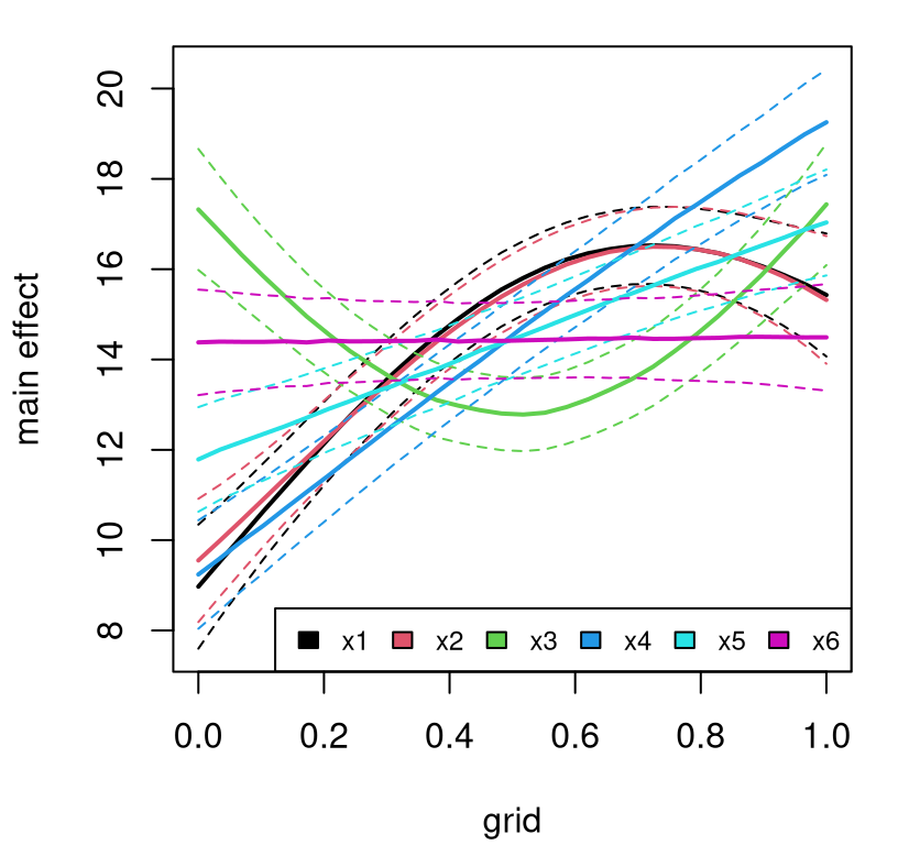

FIGURE 8.13: Main effects from Figure 8.12 augmented with quantiles.

A larger training set would drive down predictive variability and make these error-bars even narrower. Two-hundred fifty data points isn’t much in six input dimensions. Were it a gridded design, that would be equivalent to a mere three unique settings for each input. That we’re able to view a bit of nuance in mean main effects with a sample of this size is a testament to LHS design, offering more diversity in the margins than a regular grid.

8.2.3 First-order and total sensitivity

Main effects make pretty pictures but they promote a qualitative impression of variable influence. By marginalizing out other inputs, they ignore how variables work together to affect changes in the response. The most common notion of sensitivity is tied to the relationship between conditional and marginal variance for \(Y\). Variance-based methods decompose uncertainties in objective function evaluations and their surrogates into variances of conditional expectations, all with respect to \(U(x)\). These are a natural measure of output association with specific sets of variables and provide a basis upon which the importance of individual inputs may be judged.

The variance-based approach presented here is originally due to Sobol, wherein a deterministic objective function is decomposed into summands of functions on lower dimensional subsets of the input space. Consider the functional decomposition

\[ f(x_1, \dots, x_m) = f_0 + \sum_{j=1}^m f_j(x_j) +\sum_{1 \leq i < j \leq m} f_{ij}(x_j,x_i) + \cdots + f_{1,\dots,m}(x_1, \dots ,x_m). \]

When \(f\) is modeled as a stochastic process \(Y(x)\) conditional on inputs \(x\), we can develop a similar decomposition of response distributions which arise when \(Y(x)\) has been integrated over one subset of covariates \(x_J= \{x_j : j \in J\}\), where \(J \subseteq \{1,\dots,m\}\), and where the complement of this subset, \(x_{-J} =\{x_j:j\notin J\}\) is allowed to vary according to a marginalized uncertainty distribution. For example, we may study the marginal conditional expectation

\[ \mathbb{E}_{U_{-J}}\{\mu(x) \mid x_J\} = \int_{\mathcal{X}_{-J}} \mathbb{E}\{y \mid x\} u_{-J}(x_{-J}) \; dx_{-J}, \]

where the subsequent marginal uncertainty density is given by \(u_J(x_J) = \int_{\mathcal{X}_{-J}} u(x) \; d x_{-J}\). Observe that this generalizes the expectation used to define main effects (8.5).

Sobol-based sensitivity analysis attempts to decompose, and quantify, variability in \(\mathbb{E}\{y \mid x_J\}\) with respect to changes in \(x_J\) according to \(U_J(x_J)\). If \(U\) is such that inputs are uncorrelated, the variance decomposition is available as

\[ \mathbb{V}\mathrm{ar}(\mathbb{E}_{U_{-J}}\{y\mid x\}) = \sum_{j=1}^m V_j + \sum_{1 \leq i < j \leq m} V_{ij} + \cdots + V_{1,\dots,m}, \]

where \(V_j = \mathbb{V}\mathrm{ar}_{U_j}(\mathbb{E}_{U_{-j}}\{y \mid x_j\})\), \(V_{ij}=\mathbb{V}\mathrm{ar}_{U_{ij}}(\mathbb{E}_{U_{-ij}}\{y \mid x_i, x_j\}) - V_i - V_j\), and so on. When inputs are correlated this identity no longer holds, although a “less-than-or-equal-to” inequality is always true. But nevertheless it’s still useful to retain an intuitive interpretation of the \(V_J\)’s as a portion of overall marginal variance.

First-order sensitivity

With that motivation in mind, define first-order sensitivity indices as

\[\begin{equation} S_j = \frac{\mathbb{V}\mathrm{ar}_{U_j}(\mathbb{E}_{U_{-j}}\{y \mid x_j\})}{\mathbb{V}\mathrm{ar}_U(y)}, \quad j=1,\dots,m. \tag{8.6} \end{equation}\]

In words, \(S_j\) is the proportion of variability in the (mean surrogate) response attributable to the \(j^{\mathrm{th}}\) input, i.e., response sensitivity to variable main effects. As you can see, \(S_j\) is scalar, so a first-order analysis reports \(m\) numbers, which is of lower dimension than main effects, providing \(m\) functions.

Perhaps main effects could be categorized as “zeroth-order” sensitivity indices, but that sells them short because of the high dimensional, functional view they provide. Yet upon conditioning there’s no notion of variability. By replacing that grid-wise evaluation with a variance calculation – i.e., another integral – first-order sensitivities offer more global perspective wrapped in a neat package. As a proportion of variability, \(S_j\) also provides a relative notion of variable importance.

Observe that lower-case \(y\)’s are used above, even though the posterior predictive quantity \(Y(x) \mid Y_n\), as in our intended surrogate GP application, is clearly a random variable. This is to emphasize that, in calculating \(S_j\), all expectations and variances are taken with respect to uncertainty distribution \(U\). Integrating over \(y\) to extract posterior predictive means is implicit for GPs, or can be ignored in the case where \(y=f(x)\) can be probed directly and without noise. Throughout our sensitivity index presentation, inner expectations are taken over \(X_{-j} \sim U_{-j}\) and outer variances over the only remaining random quantity, \(X_j \sim U_j\). When variances/expectations are not nested, as in the variance in the denominator (8.6), integration over all of \(X \sim U\) is implied. Below we shall drop distributional subscripts \(\mathbb{V}\mathrm{ar}_{U_j}\) and \(\mathbb{E}_{U_{-j}}\) to streamline the notation, but the same principles are in play.

MC approximation of first-order indices \(S_j\) benefits from the following development. Using the definition for variance, we have

\[\begin{equation} S_j = \frac{\mathbb{E}\{\mathbb{E}^2\{y \mid x_j\}\} - \mathbb{E}^2\{y\}}{\mathbb{V}\mathrm{ar}(y)} \tag{8.7} \end{equation}\]

since \(\mathbb{E}_{U_j}^2\{\mathbb{E}_{U_{-j}}\{y\mid x_j\}\} = \mathbb{E}^2_U\{y\} \equiv \mathbb{E}^2\{y\}\). Eq. (8.7) follows (8.6) by taking inner expectation over \(X_{-j}\), and outer one over \(X_j\), combining to integrate over all of \(X \sim U\). To calculate those expectations, let \(M\) and \(M'\) be samples of size \(N\) from \(U\), e.g., from LHSs respecting \(U\), being comprised of \(m\)-length row vectors \(s_k\) and \(s'_k\), for \(k=1,\dots,N\) respectively. Approximate unconditional quantities as

\[ \widehat{\mathbb{E}\{y\}} = \frac{1}{N} \sum_{k=1}^{N}\mathbb{E}\{y \mid s_k\} \quad \mbox{ and } \quad \widehat{\mathbb{V}\mathrm{ar}(y)} = \frac{1}{N} \mathbb{E}\{y \mid M\}^\top \mathbb{E}\{y \mid M\} - \widehat{\mathbb{E}^2\{y\}}, \]

where \(\mathbb{E}\{y \mid M\}\) is the column vector \(\left[\mathbb{E}\{y \mid s_1\}, \cdots, \mathbb{E}\{y \mid s_{N}\}\right]^\top\) and \(\widehat{\mathrm{E}^2\{y\}} = \widehat{\mathbb{E}\{y\}}\widehat{\mathbb{E}\{y\}}\). Approximating the rest of \(S_j\), through conditional expectations, requires mixing columns of \(M\) with a similarly built matrix \(M'\) of \(s_k'\) conditioned columns. Independence in coordinates of \(U\) is crucial here. Let \(M_j'\) be \(M'\) with \(j^{\mathrm{th}}\) column replaced by the \(j^{\mathrm{th}}\) column of \(M\), and likewise let \(M_j\) be \(M\) with the \(j^{\mathrm{th}}\) column of \(M'\). Then, the conditional second moment required for \(S_j\) may be approximated as

\[ \widehat{\mathbb{E}\{\mathbb{E}^2\{y \mid x_j\}\}} = \frac{1}{N-1}\mathbb{E}\{y \mid M\}^\top\mathbb{E}\{y \mid M'_j\}. \]

A formal algorithm is coming shortly, but to save a little space we’ll wait until after providing details on total sensitivity indices as the two share many subroutines. First, an illustration: let’s run through the math above in code below on the Friedman data. Unconditional quantities may be approximated as follows, based on a single \(m\)-dimensional LHS \(M\) of size \(N\).

M <- randomLHS(N, 6)
pM <- predGPsep(gpi, M, lite=TRUE, nonug=TRUE)
Ey <- mean(pM$mean)
Vary <- (t(pM$mean) %*% pM$mean)/N - Ey^2

Then, using mixtures of columns of a second LHS with those of the first, approximations to conditional quantities may be combined with the unconditional ones above to estimate \(S_j\), for \(j=1,\dots,m\).

Mprime <- randomLHS(N, 6)
S <- EE2j <- rep(NA, 6)
for(j in 1:6) {
  Mjprime <- Mprime
  Mjprime[,j] <- M[,j]
  pMprime <- predGPsep(gpi, Mjprime, lite=TRUE, nonug=TRUE)
  EE2j[j] <- (t(pM$mean) %*% pMprime$mean)/(N - 1)
  S[j] <- (EE2j[j] - Ey^2)/Vary
}

Estimated first-order indices are quoted below.

S

## [1] 0.21968 0.19607 0.09642 0.37787 0.10241 0.01388

According to those numbers, our surrogate is most sensitive to input four. This agrees with Figures 8.12–8.13 providing main effects plot(s) which show \(x_4\)’s marginal response varying over the largest range of the \(y\)-axis. Given what we know about the true data generating mechanism, this summary is correct. Although input \(x_3\) (being quadratic) has the potential for bigger effect (\(x_4\)’s is but linear), that could only happen for \(|x_3 - 0.5| > 1\), lying outside the study area. Inputs \(x_1\) and \(x_2\) have the second highest first-order sensitives, being similar to one another. This too makes sense: they only work together in interaction and, as products of numbers less than one in absolute value, span a smaller range of outputs despite sharing the same amplitude as \(x_4\), namely 10.

Total sensitivity

Total sensitivity indices are the mirror image of first-order indices:

\[ T_j = \frac{\mathbb{E}\{\mathbb{V}\mathrm{ar}(y \mid x_{-j})\}}{\mathbb{V}\mathrm{ar}(y)}. \]

Observe that \(\mathbb{E}\{ \mathbb{V}\mathrm{ar}(y \mid x_{-j} ) \} = \mathbb{V}\mathrm{ar}(y) - \mathbb{V}\mathrm{ar}(\mathbb{E} \{ y \mid x_{-j} \})\), so \(T_j\) measures residual variance in conditional expectation and thus represents all influence connected to a given variable. Consequently the difference between first-order and total sensitivities, \(T_j - S_j\), measures variability in \(y\) due to the interaction between input \(j\) and the other inputs. A large difference \(T_j-S_j\) can trigger additional local analysis to determine its functional form.

Again, expanding out the definition for variance as a difference in squared expectations, we have

\[ T_j = 1 - \frac{\mathbb{E}\{\mathbb{E}^2\{y \mid x_{-j}\}\} - \mathbb{E}^2\{y\}}{\mathbb{V}\mathrm{ar}(y)}. \]

So there’s only one additional quantity required to calculate \(T_j\) beyond elements needed for \(S_j\). Similarly,

\[ \begin{aligned} \widehat{\mathbb{E}\{\mathbb{E}^2\{y \mid x_{-j}\}\}} &= \frac{1}{N-1}\mathbb{E}\{y \mid M'\}^\top\mathbb{E}\{y \mid M_j'\} \\ &\approx \frac{1}{N-1}\mathbb{E}\{y \mid M\}^\top\mathbb{E}\{y \mid M_j\}, \end{aligned} \]

with the latter approximation saving us the effort of predicting at locations in \(M'\) by re-using those on hand at \(M\).

Consider total sensitivity indices on the Friedman data.

T <- EE2mj <- rep(NA, 6)
for(j in 1:6) {
  Mj <- M
  Mj[,j] <- Mprime[,j]
  pMj <- predGPsep(gpi, Mj, lite=TRUE, nonug=TRUE)
  EE2mj[j] <- (t(pM$mean) %*% pMj$mean)/(N - 1)
  T[j] <- 1 - (EE2mj[j] - Ey^2)/Vary
}
deleteGPsep(gpi)

As shown below, input four again has the highest index, with inputs one and two close behind.

T

## [1]  0.262157  0.233274  0.087635  0.369807  0.093066 -0.002233

Although the information seems redundant, their difference can be used to order potential for interaction among pairs of input variables …

I <- T-S
I[I < 0] <- 0
I

## [1] 0.04248 0.03720 0.00000 0.00000 0.00000 0.00000

… which we know is correct from the definition of the fried function. Notice that any negative differences are thresholded above. This is to compensate for sampling variability in the MC approximation. Theoretically, \(T \geq S\) when inputs are independent under \(U\). (All bets are off for dependent inputs.) MC error, leading to negative I, can be exacerbated by one of the big drawbacks of Saltelli/Sobol analysis: first-order and total indices may fail to sum to the total variance. Although both measure a proportion, they don’t partition variability. To address this issue, Owen (2014) proposed an alternative sensitivity measure called a Shapely effect, motivated by Shapley values from game theory. Shapley effects always partition variance when inputs are independent under \(U\). Unfortunately, estimating Shapley effects can be cumbersome computationally. Song, Nelson, and Staum (2016) suggest one possible approach, as well as provide an excellent survey of the modern landscape of sensitivity estimation when there are many inputs.

So that everything is in one place, Algorithm 8.4 codifies the sequence of steps required to calculate first-order and total sensitivity indices.

Algorithm 8.4: Sobol First-Order and Total Sensitivity Indices

Assume \(m\)-dimensional inputs \(x\).

Require uncertainty distribution \(U\) which may readily be sampled, say with LHS via margins \(u_1,\dots,u_m\); a desired sample size \(N\) controlling MC accuracy; surrogate or predictive equations \(p(y \mid x)\), say from a GP, generating \(\mu(x)\).

Then

1. Draw two \(N \times m\) LHSs from \(U\), and denote these as

\[ M = \begin{pmatrix} s_{1_1} & s_{1_2} & \cdots & s_{1_m} \\ s_{2_1} & s_{2_2} & \cdots & s_{2_m} \\ \vdots & \vdots & \ddots & \vdots \\ s_{N_1} & s_{N_2} & \cdots & s_{N_m} \end{pmatrix} \quad \mbox{ and } \quad M' = \begin{pmatrix} s_{1_1}' & s_{1_2}' & \cdots & s_{1_m}' \\ s_{2_1}' & s_{2_2}' & \cdots & s_{2_m}' \\ \vdots & \vdots & \ddots & \vdots \\ s_{N_1}' & s_{N_2}' & \cdots & s_{N_m}' \end{pmatrix}. \]

2. Evaluate surrogate (GP) predictive equations at \(M\), saving mean \(N\)-vector \(\hat{y}\) with \(i^{\mathrm{th}}\) component \(\mu(s_i)\), and approximate

\[ \widehat{\mathbb{E}\{y\}} = \frac{1}{N} \sum_{i=1}^N \mu(s_i) \quad \mbox{ and } \quad \widehat{\mathbb{V}\mathrm{ar}(y)} = \frac{\hat{y}^\top \hat{y}}{N} - \widehat{\mathbb{E}^2\{y\}}. \]

For each coordinate \(x_j\) of \(x\), i.e., for \(j=1,\dots,m\), do …

3. Create column-swapped matrices \(M'_j\) and \(M_j\) from \(M\) and \(M'\) as follows

\[ M'_j = \begin{pmatrix} s_{1_1}' & \cdots & s_{1_j} & \cdots & s_{1_m}' \\ s_{2_1}' & \cdots & s_{2_j} & \cdots & s_{2_m}' \\ \vdots & \vdots & \vdots & \ddots & \vdots \\ s_{N_1}' & \cdots & s_{N_j} & \cdots & s_{N_m}' \end{pmatrix} \quad \mbox{ and } \quad M_j = \begin{pmatrix} s_{1_1} & \cdots & s_{1_j}' & \cdots & s_{1_m} \\ s_{2_1} & \cdots & s_{2_j}' & \cdots & s_{2_m} \\ \vdots & \vdots & \vdots & \ddots & \vdots \\ s_{N_1} & \cdots & s_{N_j}' & \cdots & s_{N_m} \end{pmatrix}. \]

4. Evaluate surrogate (GP) predictive equations at \(M'_j\) and \(M_j\) saving mean \(N\)-vectors \(\hat{y}'_j\) and \(\hat{y}_j\) analogous to Step 2, above, and approximate

\[ \widehat{\mathbb{E}\{\mathbb{E}^2\{y \mid x_j\}\}} = \frac{\hat{y}^\top \hat{y}'_j}{N-1} \quad \mbox{ and } \quad \widehat{\mathbb{E}\{\mathbb{E}^2\{y \mid x_{-j}\}\}} = \frac{\hat{y}^\top \hat{y}_j}{N-1}. \\ \]

5. Finally, build first-order and total indices by combining quantities calculated above as follows:

\[ S_j = \frac{\widehat{\mathbb{E}\{\mathbb{E}^2\{y \mid x_j\}\}} - \widehat{\mathbb{E}^2\{y\}}}{\widehat{\mathbb{V}\mathrm{ar}(y)} } \quad \mbox{ and } \quad T_j = 1 - \frac{\widehat{\mathbb{E}\{\mathbb{E}^2\{y \mid x_{-j}\}\}} - \widehat{\mathbb{E}^2\{y\}}}{\widehat{\mathbb{V}\mathrm{ar}(y)}}. \]

End For

Return \(m\)-vectors \(S\) and \(T\).

The set of input locations which must be evaluated under the surrogate for each calculation of indices \(S_j\) and \(T_j\) is \(\{M, M', M'_1, M_1, \dots, M'_m, M_m\}\), which is \(N(2m+2)\) in total. Saltelli’s original version involves \(N(m+2)\), almost half as many, but I find the variation in Algorithm 8.4 to be easier to explain and implement. Saltelli also recommends using an alternative estimate \(\widehat{\mathbb{E}\{y\}} = \frac{1}{N-1} \mathbb{E}\{y \mid M\}^\top \mathbb{E}\{y \mid M'\}\) in calculating first-order indices, \(S_j\), as this brings the index closer to zero for non-influential variables. In my experience, that trick can induce bias in estimates and suffer from numerical instability. Instead I prefer the simpler, default setup presented above.

LHSs \(M\) and \(M'\) can be re-used to estimate main effects, at little extra computational cost, as a byproduct of calculations required for Sobol indices. A post-processing one-dimensional nonparametric regression through the scatterplot of \([s_{1_j}, \ldots, s_{N_j},s'_{1_j}, \ldots, s'_{N_j}]\) vs. \([\mathbb{E}\{y \mid M\},\mathbb{E}\{y \mid M'\}]\) for each of \(j=1,\ldots,m\) input variables may be snapped to a grid for plotting purposes. I’ve found this approach to be quite robust to choices of smoother since \(2N\) typically represents a very large sample in 1d. For example, lowess works well in R. This technique is utilized by the tgp package (Gramacy and Taddy 2016) for fully Bayesian sensitivity and main effects, discussed in more detail momentarily.

As a final note before showcasing that library implementation, the numerical integration scheme(s) outlined above extend(s) nicely to other Sobol indices (e.g., second-order, etc.) for particular combinations of inputs. For details and further discussion, the curious reader is invited to explore some of the references offered at the start of this section (§8.2), particularly the edited volume by Saltelli, Chan, and Scott (2000). Such extensions are less common in the surrogate modeling literature.

8.2.4 Bayesian sensitivity

Now those were just point estimates – by which I mean everything we did above on main effects and first-order/total sensitivity – derived from MLE GP fits. We visualized quantiles of main effects, but that offered a higher resolution view of the concept of main effect rather than a quantification of their uncertainty. Like any quantity estimated from data, sensitivity indices have a sampling distribution. In turn, their distribution could help determine, say, which indices are indeed substantially bigger than others or bigger than some baseline like zero.

Considering the MC nature of calculations, closed form derivation of the sampling distribution of sensitivity indices is a nonstarter. One option is the bootstrap. I don’t know if this has ever been done for main, first-order and total Sobol indices with GP surrogates. The (parametric) bootstrap has been used with GP surrogates and for other applications, such as KOH-style calibration (Gramacy et al. 2015). Yet use of the bootstrap in this context, where the prevailing view is Bayesian (§5.3.2), feels like a mismatch of technologies at best, and incoherent at worst.

Sampling from the posterior distribution of all unknown quantities when surrogate modeling, including hyperparameters, is no different in principle than MCMC for calibration parameters, e.g., Algorithm 8.1. Augmenting that MCMC with an extra layer of MC over \(U\) LHSs is pretty straightforward. (Hopefully it’s not too confusing that both are notated by \(u\).) Yet implementing such a method is too cumbersome for Rmarkdown presentation here. Fortunately it’s implemented in software, in several packages actually.

Here I shall illustrate the implementation in tgp, as described by Gramacy and Taddy (2010), which is based on a flexible family of (treed) GPs. Simpler, traditional GP formulations may leverage a greater degree of analytic tractability (Oakley and O’Hagan 2004). See GPMSA software for implementation.

library(tgp)

More detail on tgp is provided in §9.2.2. Similar functionality is provided in dynaTree (Gramacy, Taddy, and Anagnostopoulos 2017) on CRAN; for more details on dynamic trees as an alternative to GPs for surrogate modeling see §9.2.3. For use in optimization and sensitivity analysis see Gramacy, Taddy, and Wild (2013). In tgp, the function sens invokes a sensitivity analysis.⁸ Providing model=bgp indicates a Bayesian GP surrogate. Argument nn.lhs is like \(N\). However the extra layer of MC offered by posterior sampling with MCMC, which by default involves \(T=4000\) iterations, allows smaller \(N\) like nn.lhs=1000 to be used compared to our earlier, pointwise, analysis. The effective number of LHS draws for \(U\) derives from their product, which in this case is 4 million.

sf <- tgp::sens(data[,1:6], data$Y, nn.lhs=1000, model=bgp, verb=0)

The tgp package provides a plot method for "tgp"-class objects, which has an optional argument layout="sens" furnishing visuals for a suite of main effects, first-order and total sensitivities. These are shown in Figure 8.14.

plot(sf, layout="sens", legendloc="topleft")

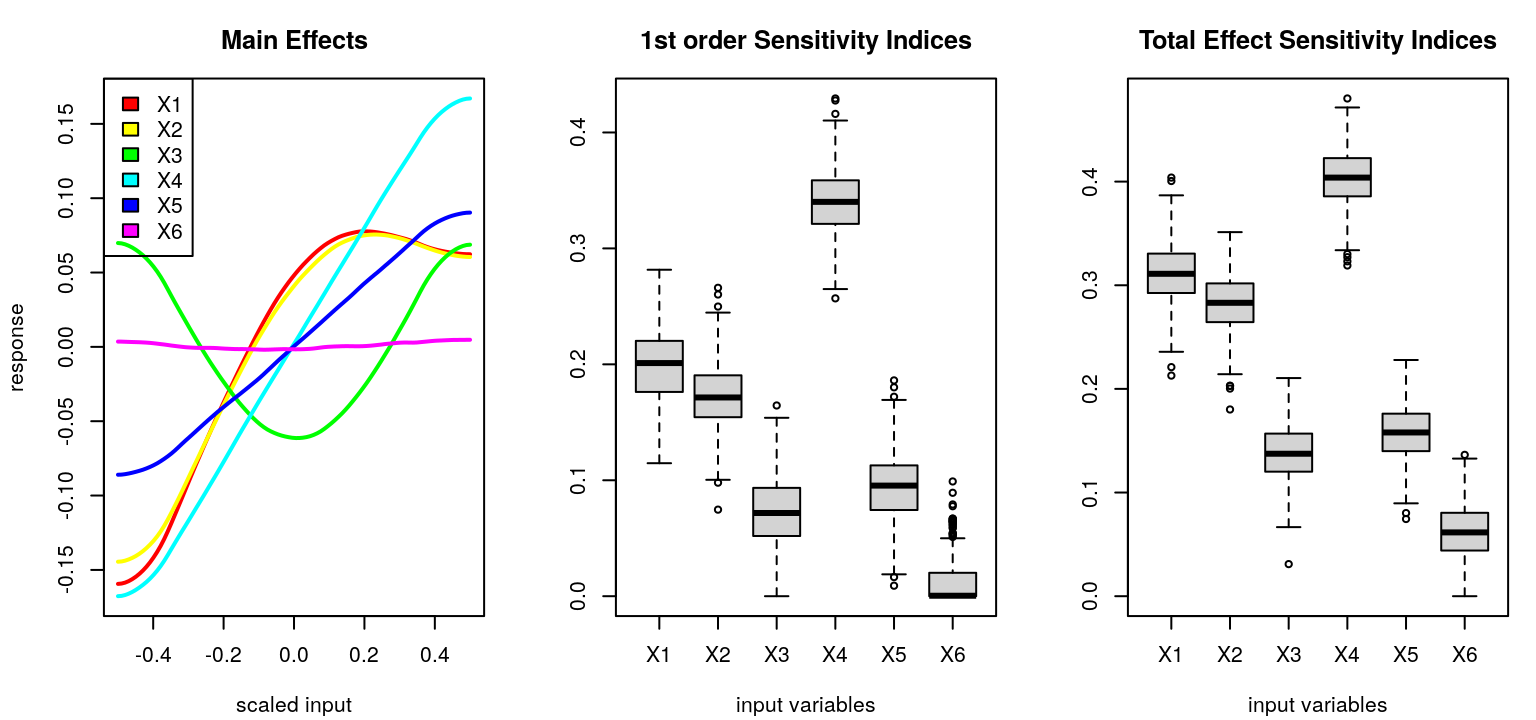
FIGURE 8.14: Summary of Bayesian sensitivity on the Friedman data.

As you can see, boxplots for first-order and total indices offer a window into posterior uncertainty in these calculations. The boxplot corresponding to first-order indices for \(x_6\) indicates not much more than 50% probability of being positive, providing strong indication that this input is not affecting the response. In fact, a common tactic is to deliberately insert a dummy, useless input like \(x_6\) to get a baseline \(S\) and \(T\) distribution through which to gauge better what might be an important effect. By default, main effects are visualized without error-bars in order to reduce clutter. An optional argument maineff allows the user to specify which inputs to view main effects on, and when that argument is provided 90% error-bars are added to the resulting plot(s). See Figure 8.15.

plot(sf, layout="sens", maineff=t(1:5))

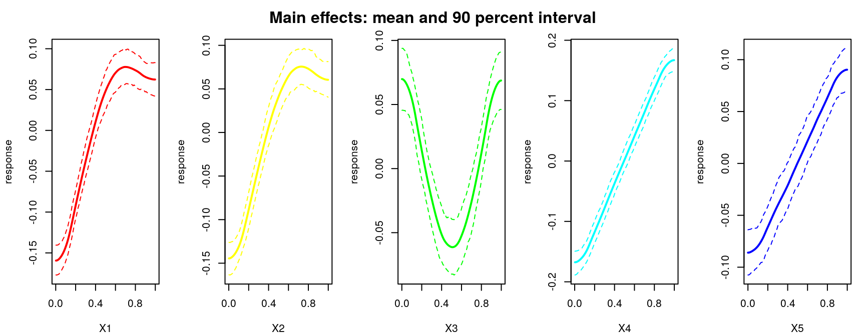
FIGURE 8.15: Bayesian main effects with error-bars on the Friedman data.

Superficially, the view here is quite similar to our mean-and-quantile point estimate-based main effects from Figure 8.13. This time, however, dashed error-bars capture full posterior uncertainty in \(Y(x)\) as each coordinate is varied while the others are integrated out.

When searching for interactions, a posterior probability can be calculated as follows.

I <- sf$sens$T - sf$sens$S
I[I < 0] <- 0
colMeans(I)

## [1] 0.11231 0.11091 0.06710 0.06451 0.06558 0.05176

Observe that \(x_1\) and \(x_2\) have the highest posterior probability of being involved in an interaction. The others are reasonably high too. One disadvantage to tgp’s implementation here is that its sampling scheme doesn’t support a nonug option. In other words, indices are calculated over \(Y(x)\) rather than \(\mu(x)\), conditional on training data. Consequently, resulting posterior summaries of sensitivity appear noisier, reflecting greater uncertainty than typically presented. A more favorable assessment would be that, as a result, they offer a conservative view by averaging over a more complete assessment of posterior variability; hence a large probability of (potential) interaction for all variables.

As another illustration, consider the airquality data in the base distribution of R. These data contain daily readings of mean ozone in parts per billion (Ozone), solar radiation (Solar.R), wind speed (Wind), and maximum temperature (Temp), for New York City between May 1 and September 30, 1973. The tgp package supports specification of Beta-distributed marginals for use in sensitivity analysis. Admittedly, this is somewhat restrictive in the landscape of statistical distributions. However, most studies focus on limited ranges for inputs, coded to the unit cube, and uncertainty distributions of interest tend to be unimodal. Beta marginals offer a relatively flexible, and straightforwardly specified, parametric family meeting that description.

Suppose we take each margin to be scaled beta with shape=2 and mode equal to the average setting for that input. Specifying a beta distribution in this way is thought to be somewhat more intuitive than the typical a and b arguments.

X <- airquality[, 2:4]
Z <- airquality$Ozone
rect <- t(apply(X, 2, range, na.rm=TRUE))
mode <- apply(X, 2, mean, na.rm=TRUE)
shape <- rep(2, 3)

This dataset has missing values. These are automatically discarded by tgp, however a warning is printed to the screen. To keep our presentation tidy, the code chunk below suppresses those warnings for the sensitivity analysis.

s.air <- suppressWarnings(tgp::sens(X=X, Z=Z, nn.lhs=300, rect=rect, 
  shape=shape, mode=mode, model=bgp, verb=0))

Figure 8.16 shows the default sensitivity layout.

plot(s.air, layout="sens")

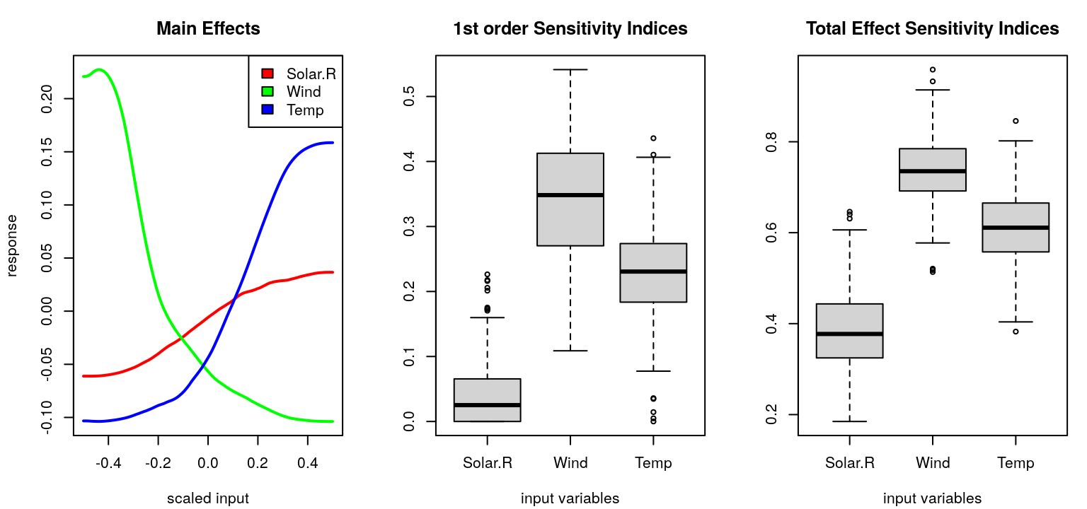
FIGURE 8.16: Sensitivity summary on the air quality data.

Main effects show nonlinear marginal relationships for all three predictors. Solar radiation has the smallest effect on the response, which is echoed in all three measurements. Wind has the largest. Differences in first and total indices indicate modest pairwise interactions among all three variables.

I <- s.air$sens$T - s.air$sens$S
I[I < 0] <- 0
colMeans(I)

## [1] 0.3434 0.3957 0.3828

More options for sensitivity analysis in tgp are detailed by Gramacy, Taddy, and Wild (2013), with supplements in the package documentation.

Hopefully the illustration herein offers a glimpse into what’s possible by pairing surrogate modeling with a generous helping of Monte Carlo integration, supporting a curiosity to tinker so long as one has the patience to let it all run. Sensitivity analysis and calibration are numerical procedures which attempt to salvage, or squeeze out, a degree of interpretability from an otherwise opaque nonparametric predictor. Often the great flexibility offered by surrogates, like those based on GPs, thwarts concrete statements derived from inference through optimization and sampling. Critics rightly point to identifiability concerns, for example. Yet much insight can be gleaned from these “beasts” with a few simple tools. That is, until the data get big …

8.3 Homework exercises

A sample of exercises on calibration and sensitivity analysis follows. Most of these focus on calibration, as there’s rather more to explore there – fewer implementations left to libraries.

#1: Calibration with free computer model simulation

Revisit the ball dropping calibration example from §8.1.2 Figure 8.1, with field data in ball.csv. Assume that the computer model timedrop is free to evaluate for any height and gravity parameter(s). Specifically, there’s no need to fit a surrogate, and thus the setup follows Higdon’s special case of the KOH framework (8.1)–(8.2).

1. Develop a calibration apparatus for this situation. In your description, be clear about what quantities are being modeled and how they’re being estimated. As in the chapter, provide two versions: (i) one where discrepancy between the computer model and field data is estimated; and (ii) where discrepancy is assumed to be zero.
2. Implement both versions (i–ii) and carry out an analysis that reports on the estimated calibration parameter, \(\hat{g}\), in natural units.
3. Provide predictions for time(s) as a function of height for both versions (i–ii) which fully propagates all uncertainties, excepting ones due to hyperparameters (e.g., lengthscales and nuggets to GPs).
4. Finally, re-implement the cross validation (CV) exercise and compare the two methods based on their proper scores. Report the jackknife sampling distribution for \(\hat{g}\) in both cases and comment.

#2: Calibration and sensitivity in 2d

Consider the following mathematical description of a computer model via inputs \(x \in [0,1]^2\) and calibration parameter \(u \in [0,1]^2\):

\[ y^M(x, u) = \left(1-e^{-\frac{1}{2x_2}}\right) \frac{1000 u_1 x_1^3 + 1900 x_1^2+2092 x_1+60}{100 u_2 x_1^3 + 500 x_1^2 + 4x_1+20}. \]

Now suppose that field data are generated as

\[ \begin{aligned} Y^F(x) &= y^M(x, u^\star) + b(x) + \varepsilon, \;\; \mbox{ where } \; b(x) = \frac{10x_1^2+4x_2^2}{50 x_1 x_2+10} \;\; \mbox{ and } \; \varepsilon \stackrel{\mathrm{iid}}{\sim} \mathcal{N}(0, 0.25^2), \end{aligned} \]

using \(u^\star=(0.2, 0.1)\). See §9.3.6 for implementation in R.

1. Generate an LHS of size 500 in four-dimensional \((x,u)\)-space and evaluate the computer model at those locations. Based on those runs, provide visualizations of main effects, first-order, and total sensitivity indices for each of the four variables.
2. Create a field data design \(X_{n_F}\) under a 2d LHS of size 50 and two replicates at each location so that \(n_F = 100\). Then obtain \(\hat{u}\) estimates under both the bias corrected and nobias modularized KOH calibration apparatus. Use a \(\mathrm{Beta}(2, 2)\) prior independently on the margins of \(u\) and GP predictors throughout. How do your \(\hat{u}\) estimates compare to the true \(u^\star\) value?
3. Generate a testing set of \(y^R(x)\)-values (i.e., without noise), under 2d LHS of size \(N_R = 1000\). Which of your two calibrated predictors, bias corrected and nobias, yield better scores on the testing set?
4. Suppose you were to use the true \(u^\star\) value in place of \(\hat{u}\), in both bias corrected and nobias alternatives above. How do the resulting “oracle-calibrated” scores compare to the ones you calculated above. Are you at all surprised by the results?

#3: Bayesian version of #2

Revisit exercise #2b with a more fully Bayesian treatment (§8.1.5), ideally using the same data. Compare the posterior distribution for \(u\) with the point estimate \(\hat{u}\) you obtained in #2. As above, use a \(\mathrm{Beta}(2,2)\) prior independently on the margins of \(u\).

#4: KOH (Bayesian) prediction

In the KOH framework, …

1. … derive the posterior predictive distribution \(Y^F(\mathcal{X}) \mid [Y_{n_M}, Y_{n_F}], u\) conditional on all other hyperparameters defining the GPs for surrogate and bias. Use MVN conditional identities similar to those involved in prediction with ordinary GPs (5.2).
2. Implement that predictor in the context of the (four-dimensional \((x,u)\)) exercises #2c and #3 above, simultaneously averaging over all \(u^{(t)}\) sampled from the posterior. Or, if you haven’t worked on those exercises, similarly extend the Bayesian analysis of the ball drop example (§8.1.5). Report predictive uncertainty on the testing set (#2c, or the grid from the chapter) and compare these to Figure 8.6 obtained from the modular optimization framework. Your comparison should be both qualitative, and quantitative (i.e., compared to the truth).

#5: Sensitivity in high dimension

Oakley and O’Hagan (2004) consider a fifteen dimensional problem whose specification includes five variables having a substantial effect on the response, five with a smaller effect, and five with almost no contribution. Fit a separable GP to responses obtained on a size-250 maximin LHS (§4.3) in fifteen dimensions. Note that your estimated lengthscales should be quite long (if you allow them to be). Use predictive equations from that fit to visualize main effects and calculate first-order sensitivity indices \(S_j\), for \(j=1,\dots,15\). (No \(T_j\) are required since Oakley & O’Hagan didn’t present those.) You may need to increase the MC size \(N\) due to the much higher dimensional input space. See if you can partition inputs into three “effect classes” of five based on main effects and first-order indices. Compare your results to Table 1 from Oakley and O’Hagan (2004). Note that they used \(U_i \equiv \mathcal{N}(0,1)\). Contrast with the fully Bayesian alternative provided by tgp. Be careful about how you “map” a Gaussian uncertainty distribution to tgp’s Beta(s); longer MCMC than the sens default may be needed due to the higher dimensional space. You may fix a small nugget by providing nug.p=0 and gd=c(0.0001, 0.1) to sens.

References

Ba, S, and VR Joseph. 2012. “Composite Gaussian Process Models for Emulating Expensive Functions.” The Annals of Applied Statistics 6 (4): 1838–60.

Berger, JO, V De Oliveira, and B Sansó. 2001. “Objective Bayesian Analysis of Spatially Correlated Data.” Journal of the American Statistical Association 96 (456): 1361–74.

Bornn, L, G Shaddick, and JV Zidek. 2012. “Modeling Nonstationary Processes Through Dimension Expansion.” Journal of the American Statistical Association 107 (497): 281–89.

Brynjarsdóttir, J, and A O’Hagan. 2014. “Learning about Physical Parameters: The Importance of Model Discrepancy.” Inverse Problems 30 (11): 114007.

Carmassi, M. 2018. CaliCo: Code Calibration in a Bayesian Framework. https://CRAN.R-project.org/package=CaliCo.

Cox, DD, JS Park, and CE Singer. 2001. “A Statistical Method for Tuning a Computer Code to a Data Base.” Computational Statistics & Data Analysis 37 (1): 77–92.

Craig, PS, M Goldstein, AH Seheult, and JA Smith. 1996. “Bayes Linear Strategies for Matching Hydrocarbon Reservoir History.” Bayesian Statistics 5: 69–95.

Da Veiga, S, F Wahl, and F Gamboa. 2009. “Local Polynomial Estimation for Sensitivity Analysis on Models with Correlated Inputs.” Technometrics 51 (4): 452–63.

DiDonato, AR, and AH Morris Jr. 1986. “Computation of the Incomplete Gamma Function Ratios and Their Inverse.” ACM Transactions on Mathematical Software 12 (4): 377–93.

Gattiker, J, K Myers, B Williams, D Higdon, M Carzolio, and A Hoegh. 2016. “Gaussian Process-Based Sensitivity Analysis and Bayesian Model Calibration with GPMSA.” Handbook of Uncertainty Quantification, 1–41.

Gneiting, T, and AE Raftery. 2007. “Strictly Proper Scoring Rules, Prediction, and Estimation.” Journal of the American Statistical Association 102 (477): 359–78.

Gramacy, RB, D Bingham, JP Holloway, MJ Grosskopf, CC Kuranz, E Rutter, M Trantham, and R Drake. 2015. “Calibrating a Large Computer Experiment Simulating Radiative Shock Hydrodynamics.” The Annals of Applied Statistics 9 (3): 1141–68.

Gramacy, RB, and MA Taddy. 2010. “Categorical Inputs, Sensitivity Analysis, Optimization and Importance Tempering with tgp Version 2, an R Package for Treed Gaussian Process Models.” Journal of Statistical Software 33 (6): 1–48.

Gramacy, RB, and MA Taddy. 2016. tgp: Bayesian Treed Gaussian Process Models. https://CRAN.R-project.org/package=tgp.

Gramacy, RB, MA Taddy, and C Anagnostopoulos. 2017. dynaTree: Dynamic Trees for Learning and Design. https://CRAN.R-project.org/package=dynaTree.

Gramacy, RB, MA Taddy, and SM Wild. 2013. “Variable Selection and Sensitivity Analysis Using Dynamic Trees, with an Application to Computer Code Performance Tuning.” The Annals of Applied Statistics 7 (1): 51–80.

Gu, M. 2019. “Jointly Robust Prior for Gaussian Stochastic Process in Emulation, Calibration and Variable Selection.” Bayesian Analysis 14 (3): 857–85.

Gu, M, and L Wang. 2018. “Scaled Gaussian Stochastic Process for Computer Model Calibration and Prediction.” SIAM/ASA Journal on Uncertainty Quantification 6 (4): 1555–83.

Hankin, RKS. 2013. BACCO: Bayesian Analysis of Computer Code Output. https://CRAN.R-project.org/package=BACCO.

Higdon, D, M Kennedy, JC Cavendish, JA Cafeo, and RD Ryne. 2004. “Combining Field Data and Computer Simulations for Calibration and Prediction.” SIAM Journal on Scientific Computing 26 (2): 448–66.

Hoff, PD. 2009. A First Course in Bayesian Statistical Methods. Vol. 580. New York, NY: Springer.

Johnson, LR, RB Gramacy, J Cohen, E Mordecai, C Murdock, J Rohr, SJ Ryan, AM Stewart-Ibarra, and D Weikel. 2018. “Phenomenological Forecasting of Disease Incidence Using Heteroskedastic Gaussian Processes: A Dengue Case Study.” The Annals of Applied Statistics 12 (1): 27–66.

Joseph, VR. 2006. “Limit Kriging.” Technometrics 48 (4): 458–66.

Kass, RE, BP Carlin, A Gelman, and RM Neal. 1998. “Markov Chain Monte Carlo in Practice: A Roundtable Discussion.” The American Statistician 52 (2): 93–100.

Kennedy, MC, and A O’Hagan. 2001. “Bayesian Calibration of Computer Models.” Journal of the Royal Statistical Society: Series B (Statistical Methodology) 63 (3): 425–64.

Liu, F, MJ Bayarri, and JO Berger. 2009. “Modularization in Bayesian Analysis, with Emphasis on Analysis of Computer Models.” Bayesian Analysis 4 (1): 119–50.

Marrel, A, B Iooss, B Laurent, and O Roustant. 2009. “Calculations of Sobol Indices for the Gaussian Process Metamodel.” Reliability Engineering & System Safety 94 (3): 742–51.

Morris, RD, A Kottas, MA Taddy, R Furfaro, and BD Ganapol. 2008. “A Statistical Framework for the Sensitivity Analysis of Radiative Transfer Models.” IEEE Transactions on Geoscience and Remote Sensing 46 (12): 4062–74.

Oakley, JE, and A O’Hagan. 2004. “Probabilistic Sensitivity Analysis of Complex Models: A Bayesian Approach.” Journal of the Royal Statistical Society: Series B (Statistical Methodology) 66 (3): 751–69.

Owen, AB. 2014. “Sobol Indices and Shapley Value.” SIAM/ASA Journal on Uncertainty Quantification 2 (1): 245–51.

Plumlee, M. 2017. “Bayesian Calibration of Inexact Computer Models.” Journal of the American Statistical Association 112 (519): 1274–85.

Saltelli, A. 2002. “Making Best Use of Model Evaluations to Compute Sensitivity Indices.” Computer Physics Communications 145 (2): 280–97.

Saltelli, A, K Chan, and M Scott. 2000. Sensitivity Analysis. New York, NY: John Wiley & Sons.

Saltelli, A, and S Tarantola. 2002. “On the Relative Importance of Input Factors in Mathematical Models: Safety Assessment for Nuclear Waste Disposal.” Journal of the American Statistical Association 97 (459): 702–9.

Santner, TJ, BJ Williams, and W Notz. 2003. The Design and Analysis of Computer Experiments, First Edition. Springer–Verlag.

Santner, TJ, BJ Williams, and W Notz. 2018. The Design and Analysis of Computer Experiments, Second Edition. New York, NY: Springer–Verlag.

Sherlock, C, P Fearnhead, and GO Roberts. 2010. “The Random Walk Metropolis: Linking Theory and Practice Through a Case Study.” Statistical Science 25 (2): 172–90.

Sobol, IM. 1993. “Sensitivity Analysis for Non-Linear Mathematical Models.” Mathematical Modelling and Computational Experiment 1: 407–14.

Sobol, IM. 2001. “Global Sensitivity Indices for Nonlinear Mathematical Models and Their Monte Carlo Estimates.” Mathematics and Computers in Simulation 55 (1-3): 271–80.

Song, E, BL Nelson, and J Staum. 2016. “Shapley Effects for Global Sensitivity Analysis: Theory and Computation.” SIAM/ASA Journal on Uncertainty Quantification 4 (1): 1060–83.

Storlie, CB, and JC Helton. 2008. “Multiple Predictor Smoothing Methods for Sensitivity Analysis: Description of Techniques.” Reliability Engineering & System Safety 93 (1): 28–54.

Storlie, CB, LP Swiler, JC Helton, and CJ Sallaberry. 2009. “Implementation and Evaluation of Nonparametric Regression Procedures for Sensitivity Analysis of Computationally Demanding Models.” Reliability Engineering & System Safety 94 (11): 1735–63.

Taddy, MA, HKH Lee, GA Gray, and JD Griffin. 2009. “Bayesian Guided Pattern Search for Robust Local Optimization.” Technometrics 51 (4): 389–401.

Tuo, R, and CF Wu. 2016. “A Theoretical Framework for Calibration in Computer Models: Parametrization, Estimation and Convergence Properties.” SIAM/ASA Journal on Uncertainty Quantification 4 (1): 767–95.

Tuo, R, and CFJ Wu. 2015. “Efficient Calibration for Imperfect Computer Models.” The Annals of Statistics 43 (6): 2331–52.

Vernon, I, M Goldstein, and RG Bower. 2010. “Galaxy Formation: A Bayesian Uncertainty Analysis.” Bayesian Analysis 5 (4): 619–69.

Welch, WJ, RJ Buck, J Sacks, HP Wynn, TJ Mitchell, and MD Morris. 1992. “Screening, Predicting, and Computer Experiments.” Technometrics 34 (1): 15–25.

Williamson, D, M Goldstein, L Allison, A Blaker, P Challenor, L Jackson, and K Yamazaki. 2013. “History Matching for Exploring and Reducing Climate Model Parameter Space Using Observations and a Large Perturbed Physics Ensemble.” Climate Dynamics 41 (7-8): 1703–29.

---

6. Some go so far as to suggest that one should not fit a KOH-type model without having informative prior information on \(u\), \(b(\cdot)\), or both.↩︎

7. Tuo and Wu (2016) prefer a so-called native norm instead.↩︎

8. The tgp package defines sens as an ordinary function, but dynaTree treats it as an identically named S3 method. To avoid confusion and runtime errors, explicit tgp::sens calls are used for code chunks in this chapter. In your own R session the tgp:: prefix is only required if dynaTree is also loaded.↩︎