Chapter 7 Optimization
In this chapter, the goal is to demonstrate how Gaussian process (GP) surrogate modeling can assist in optimizing a blackbox objective function. That is, a function about which one knows little – one opaque to the optimizer – and that can only be probed through expensive evaluation. We view optimization as an example of sequential design or active learning (§6.2). Many names have been given to this enterprise, and some will be explained alongside their origins below. Recently Bayesian Optimization (BO) has caught on, especially in the machine learning (ML) community, and likely that’ll stick in part because it’s punchier than the alternatives. BO terminology goes back to a paper predating use of GPs toward this end, and refers primarily to decision criteria for sequential selection and model updating. Modern ML vernacular prefers acquisition functions. BO’s recent gravitas is primarily due to the prevailing view of GP learning as marginalization over a latent random field (§5.3.2).
The role of modeling in optimization, more generically, has a rich history, and we’ll barely scratch the surface here. Models deployed to assist in optimization can be both statistical and non-statistical, however the latter often have strikingly similar statistical analogs. Potential for modern nonparametric statistical surrogate modeling in this context is just recently being recognized by communities for which optimization is bread-and-butter: mathematical programming, statistics, ML, and more. Optimization has played a vital role in stats and ML for decades. All those "L-BFGS-B" searches (Byrd et al. 1995) from optim in earlier chapters, say to find MLEs or optimal designs, are cases in point. It’s intriguing to wonder whether statistical thinking might have something to give back to the optimization world, as it were.
Whereas many communities have long settled for local refinement, statistical methods based on nonparametric surrogate models offer promise for greater scope. True global optimization, whatever that means, may always remain elusive and enterprises motivated by such lofty goals may be folly. But anyone suggesting that wider perspective is undesirable, and that systematic frameworks developed toward that end aren’t worth exploring, is ignoring practitioners and clients who are optimistic that the grass is greener just over the horizon.
Statistical decision criteria can leverage globally scoped surrogates to balance exploration (uncertainty reduction; Chapter 6) and exploitation (steepest ascent; Chapter 3) in order to more reliably find global optima. But that’s just the tip of the iceberg. Statistical models cope handily with noisy blackbox evaluations – a situation where probabilistic reasoning ought to have a monopoly – and thus lend a sense of robustness to solutions and to a notion of convergence. They offer the means of uncertainty quantification (UQ) about many aspects, including the chance that local or global optima were missed. Extension to related, optimization-like criteria such as level-set/contour finding (e.g., Ranjan, Bingham, and Michailidis 2008) is relatively straightforward, although these topics aren’t directly addressed in this chapter. See §10.3.4 for pointers along these lines.
It’s important to disclaim that thinking statistically need not preclude application of more classical approaches. Surrogate modeling naturally lends itself to hybridization. Ideas from mathematical programming not only have merit, but their software is exceedingly well engineered. Let’s not throw the baby out with the bath water. It makes sense to borrow strengths from multiple toolkits and leverage solid implementation and decades of stress testing.
Although the main ideas on statistical surrogate modeling for optimization originate in the statistics literature, it’s again machine learners who are making the most noise in this area today. This is, in part, because they’re more keen to adopt the rich language of mathematical programming, and therefore better able to connect with the wider optimization community. Statisticians tend to get caught up in modeling details and forget that optimization is as much about execution as it’s about methodology. Practitioners want to use these tools, but rarely have the in-house expertise required to code them up on their own. General purpose software leveraging surrogates has been slow to come online. An important goal of this chapter is to show how that might work, and to expose substantial inroads along those lines.
We’ll see how modern nonparametric surrogate modeling and clever (yet arguably heuristic) criteria, that often can be solved in closed form, may be combined to effectively balance exploration and exploitation. Emphasis here is on GPs, but many methods are agnostic to choices of surrogate. We begin by targeting globally scoped numerical optimization, leveraging only blackbox evaluations of an objective function supplied by the user. Subsequently, we shall embellish that setup with methods for handling constraints, known and unknown (i.e., also blackbox); hybridize with modern methods from mathematical programming; and talk about applications from toy to real data.
7.1 Surrogate-assisted optimization
Statistical methods in optimization, in particular of noisy blackbox functions, probably goes back to Box and Draper (1987), a precursor to a canonical response surface methods text by the same authors (Box and Draper 2007). Modern Bayesian optimization (BO) is closest in spirit to methods described by Mockus, Tiesis, and Zilinskas (1978) in a paper entitled “The application of Bayesian methods for seeking the extremum”. Yet many strategies suggested therein didn’t come to the fore until the late 1990’s, perhaps because they emphasized rather crude (linear) modeling. As GPs became established for modeling computer simulations, and subsequently in ML in the 2000s, new life was breathed in.
In the computer experiments literature, folks have been using GPs to optimize functions for some time. One of the best references for the core idea might be Booker et al. (1999), with many ingredients predating that paper. They called it surrogate-assisted optimization, and it involved a nice collaboration between optimization and computer modeling researchers. Non-statistical surrogates had been in play in optimization for some time. Nonparametric statistical ones, with more global scope, offered fresh perspective.
The methodology is simple: train a GP on function evaluations obtained so far; minimize the fitted surrogate predictive mean surface of the GP to select the next location for evaluation; repeat. This is an instance of Algorithm 6.1 in §6.2 where the criterion \(J(x)\) in Step 3 is based on GP predictive mean \(\mu_n(x) = \mathbb{E}\{Y(x) \mid D_n\}\) provided in Eq. (5.2). Although Step 3 deploys its own inner-optimization, minimizing \(\mu_n(x)\) is comparatively easy since it doesn’t involve evaluating a computationally intensive, and potentially noisy, blackbox. It’s something that can easily be solved with conventional methods. As a shorthand, and to connect with other acronyms like EI and PI below, I shall refer to this “mean criterion” as the EY heuristic for surrogate-assisted (Bayesian) optimization (BO).
Before we continue, let’s be clear about the problem. Whereas the RSM literature (Chapter 3) orients toward maxima, BO and math programming favor minimization, which I shall adopt for our discussions here. Specifically, we wish to find
\[ x^\star = \mathrm{argmin}_{x \in \mathcal{X}} \; f(x) \]
where \(\mathcal{X}\) is usually a hyperrectangle, a bounding box, or another simply constrained region. We don’t have access to derivative evaluations for \(f(x)\), nor do we necessarily want them (or want to approximate them) because that could represent additional substantial computational expense. As such, methods described here fall under the class of derivative-free optimization. See, e.g., Conn, Scheinberg, and Vicente (2009), for which many innovative algorithms have been proposed, and many solid implementations are widely available. For a somewhat more recent review, including several of the surrogate-assisted/BO methods introduced here, see Larson, Menickelly, and Wild (2019).
All we get to do is evaluate \(f(x)\), which for now is presumed to be deterministic. Generalizations will come after introducing main concepts, including simple extensions for the noisy case. The literature targets scenarios where \(f(x)\) is expensive to evaluate (in terms of computing time, say), but otherwise is well-behaved: continuous, relatively smooth, only real-valued inputs, etc. Again, these are relaxable modulo suitable surrogate and/or kernel structure. Several appropriate choices are introduced in later chapters.
Implicit in the computational expense of \(f(x)\) evaluations is a tacit “constraint” on the solver, namely that it minimize the number of such evaluations. Although it’s not uncommon to study aspects of convergence in these settings, often the goal is simply to find the best input, \(x^\star\) minimizing \(f\), in the fewest number of evaluations. So in empirical comparisons we typically track the best objective value (BOV) found as a function of the number of blackbox evaluations. In many applied contexts it’s more common to have a fixed evaluation budget than it is to enjoy the luxury of running to convergence. Nevertheless, monitoring progress plays a key role when deciding if further expensive evaluations may be required.
7.1.1 A running example
Consider an implementation of Booker et al.’s method on a re-scaled/coded version of the Goldstein–Price function. See §1.4 homework exercises for more on this challenging benchmark problem.
f <- function(X)
 {
  if(is.null(nrow(X))) X <- matrix(X, nrow=1)
  m <- 8.6928
  s <- 2.4269
  x1 <- 4*X[,1] - 2
  x2 <- 4*X[,2] - 2
  a <- 1 + (x1 + x2 + 1)^2 *
    (19 - 14*x1 + 3*x1^2 - 14*x2 + 6*x1*x2 + 3*x2^2)
  b <- 30 + (2*x1 - 3*x2)^2 *
    (18 - 32*x1 + 12*x1^2 + 48*x2 - 36*x1*x2 + 27*x2^2)
  f <- log(a*b)
  f <- (f - m)/s
  return(f)
 }
Although this \(f(x)\) isn’t opaque to us, and not expensive to evaluate, we shall treat it as such for purposes of illustration. Not much insight can be gained by looking at its form in any case, except to convince the reader that it furnishes a suitably complicated surface despite residing in modest input dimension (\(m=2\)).
Begin with a small space-filling Latin hypercube sample (LHS; §4.1) seed design in 2d.
Next fit a separable GP to those data, with a small nugget for jitter. All of the same caveats about initial lengthscales in GP-based active learning – see §6.2.1 – apply here. To help create a prior on \(\theta\) that’s more stable, darg below utilizes a large auxiliary pseudo-design in lieu of X, which at early stages of design/optimization (\(n_0 = 12\) runs) may not yet possess a sufficient diversity of pairwise distances.
library(laGP)
da <- darg(list(mle=TRUE, max=0.5), randomLHS(1000, 2))
gpi <- newGPsep(X, y, d=da$start, g=1e-6, dK=TRUE)
mleGPsep(gpi, param="d", tmin=da$min, tmax=da$max, ab=da$ab)$msg
## [1] "CONVERGENCE: REL_REDUCTION_OF_F <= FACTR*EPSMCH"Just like our ALM/C searches from §6.2, consider an objective based on GP predictive equations. This represents an implementation of Step 3 in Algorithm 6.1 for sequential design/active learning, setting EY as sequential design criterion \(J(x)\), or defining the acquisition function in ML jargon.
Now the predictive mean surface (like \(f\), through the evaluations it’s trained on) may have many local minima, but let’s punt for now on the ideal of global optimization of EY – of the so-called “inner loop” – and see where we get with a search initialized at the current best value. R code below extracts that value: m indexing the best y-value obtained so far, and uses its \(x\) coordinates to initialize a "L-BFGS-B" solver on obj.mean.
m <- which.min(y)
opt <- optim(X[m,], obj.mean, lower=0, upper=1, method="L-BFGS-B", gpi=gpi)
opt$par
## [1] 0.4175 0.2481So this is the next point to try. Surrogate optima represent a sensible choice for the next evaluation of the expensive blackbox, or so the thinking goes. Before moving to the next acquisition, Figure 7.1 provides a visualization. Open circles indicate locations of the size-\(n_0\) LHS seed design. The origin of the arrow indicates X[m,]: the location whose y-value is lowest based on those initial evaluations. Its terminus shows the outcome of the optim call: the next point to try.
plot(X[1:ninit,], xlab="x1", ylab="x2", xlim=c(0,1), ylim=c(0,1))
arrows(X[m,1], X[m,2], opt$par[1], opt$par[2], length=0.1)
FIGURE 7.1: First iteration of EY-based search initialized from the value of the objective obtained so far.
Ok, now evaluate \(f\) at opt$par, update the GP and its hyperparameters …
ynew <- f(opt$par)
updateGPsep(gpi, matrix(opt$par, nrow=1), ynew)
mle <- mleGPsep(gpi, param="d", tmin=da$min, tmax=da$max, ab=da$ab)
X <- rbind(X, opt$par)
y <- c(y, ynew)
… and solve for the next point.
m <- which.min(y)
opt <- optim(X[m,], obj.mean, lower=0, upper=1, method="L-BFGS-B", gpi=gpi)
opt$par
## [1] 0.4930 0.2661Figure 7.2 shows what that looks like in the input domain, as an update on Figure 7.1. In particular, the terminus of the arrow in Figure 7.1 has become an open circle in Figure 7.2, as that input–output pair has been promoted into the training data with GP fit revised accordingly.
plot(X, xlab="x1", ylab="x2", xlim=c(0,1), ylim=c(0,1))
arrows(X[m,1], X[m,2], opt$par[1], opt$par[2], length=0.1)
FIGURE 7.2: Second iteration of EY search following Figure 7.1.
If the origin of the new arrow resides at the newly minted open circle, then we have progress: the predictive mean surface was accurate and indeed helpful in finding a new best point, minimizing \(f\). If not, then the origin is back at the same open circle it originated from before.
Now incorporate the new point into our dataset and update the GP predictor.
ynew <- f(opt$par)
updateGPsep(gpi, matrix(opt$par, nrow=1), ynew)
mle <- mleGPsep(gpi, param="d", tmin=da$min, tmax=da$max, ab=da$ab)
X <- rbind(X, opt$par)
y <- c(y, ynew)
Let’s fast-forward a little bit. Code below wraps what we’ve been doing above into a while loop with a simple check on convergence in order to “break out”. If two outputs in a row are sufficiently close, within a tolerance 1e-4, then stop. That’s quite crude, but sufficient for illustrative purposes.
while(1) {
  m <- which.min(y)
  opt <- optim(X[m,], obj.mean, lower=0, upper=1,
    method="L-BFGS-B", gpi=gpi)
  ynew <- f(opt$par)
  if(abs(ynew - y[length(y)]) < 1e-4) break
  updateGPsep(gpi, matrix(opt$par, nrow=1), ynew)
  mle <- mleGPsep(gpi, param="d", tmin=da$min, tmax=da$max, ab=da$ab)
  X <- rbind(X, opt$par)
  y <- c(y, ynew)
}
deleteGPsep(gpi)
To help measure progress, code below implements some post-processing to track the best y-value (bov: best objective value) over those iterations. The function is written in some generality in order to accommodate application in several distinct settings, coming later.
bov <- function(y, end=length(y))
 {
  prog <- rep(min(y), end)
  prog[1:min(end, length(y))] <- y[1:min(end, length(y))]
  for(i in 2:end)
    if(is.na(prog[i]) || prog[i] > prog[i-1]) prog[i] <- prog[i-1]
  return(prog)
 }
In our application momentarily, note that we treat the \(n_0 = 12\) seed design the same as later acquisitions, even though they were not derived from the surrogate/criterion.
That progress meter is shown visually in Figure 7.3. A vertical dashed line indicates \(n_0\), the size of seed LHS design.
plot(prog, type="l", col="gray", xlab="n: blackbox evaluations",
  ylab="best objective value")
abline(v=ninit, lty=2)
legend("topright", "seed LHS", lty=2, bty="n")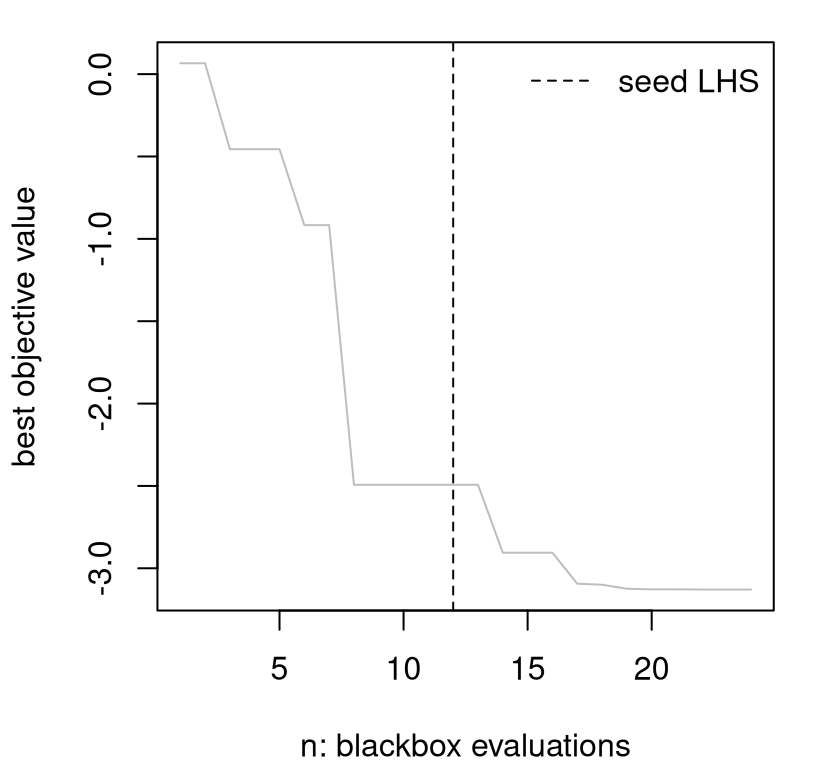
FIGURE 7.3: EY progress in terms of BOV over sequential design iterations.
Although it’s difficult to comment on particulars due to random initialization, in most variations substantial progress is apparent over the latter 12 iterations of active learning. There may be plateaus where consecutive iterations show no progress, but these are usually interspersed with modest “drops” and even large “plunges” in BOV. When comparing optimization algorithms based on such progress metrics, the goal is to have BOV curves hug the lower-left-hand corner of the plot to the greatest extent possible: to have the best value of the objective in the fewest number of iterations/evaluations of the expensive blackbox.
To better explore diversity in progress over repeated trials with different random seed designs, an R function below encapsulates our code from above. In addition to a tolerance on successive y-values, an end argument enforces a maximum number of iterations. The full dataset of inputs X and evaluations y is returned.
optim.surr <- function(f, m, ninit, end, tol=1e-4)
 {
  ## initialization
  X <- randomLHS(ninit, m)
  y <- f(X)
  da <- darg(list(mle=TRUE, max=0.5), randomLHS(1000, m))
  gpi <- newGPsep(X, y, d=da$start, g=1e-6, dK=TRUE)
  mleGPsep(gpi, param="d", tmin=da$min, tmax=da$max, ab=da$ab)

  ## optimization loop
  for(i in (ninit+1):end) {
    m <- which.min(y)
    opt <- optim(X[m,], obj.mean, lower=0, upper=1,
      method="L-BFGS-B", gpi=gpi)
    ynew <- f(opt$par)
    if(abs(ynew - y[length(y)]) < tol) break
    updateGPsep(gpi, matrix(opt$par, nrow=1), ynew)
    mleGPsep(gpi, param="d", tmin=da$min, tmax=da$max, ab=da$ab)
    X <- rbind(X, opt$par)
    y <- c(y, ynew)
  }

  ## clean up and return
  deleteGPsep(gpi)
  return(list(X=X, y=y))
 }
Consider re-seeding and re-solving the optimization problem, minimizing f, in this way over 100 Monte Carlo (MC) repetitions. The loop below combines calls to optim.surr with prog post-processing. A maximum number of end=50 iterations is allowed, but often convergence is signaled after many fewer acquisitions.
reps <- 100
end <- 50
prog <- matrix(NA, nrow=reps, ncol=end)
for(r in 1:reps) {
  os <- optim.surr(f, 2, ninit, end)
  prog[r,] <- bov(os$y, end)
}
It’s important to note that these are random initializations, not random searches. Searches (after initialization) are completely deterministic. Surrogate-assisted/Bayesian optimization is not a stochastic optimization, like simulated annealing, although sometimes deterministic optimizers are randomly initialized as we have done here. Stochastic optimizations, where each sequential decision involves a degree of randomness, don’t make good optimizers for expensive blackbox functions because random evaluations of \(f\) are considered too wasteful in computational terms.
Figure 7.4 shows the 100 trajectories stored in prog.
matplot(t(prog), type="l", col="gray", lty=1,
  xlab="n: blackbox evaluations",  ylab="best objective value")
abline(v=ninit, lty=2)
legend("topright", "seed LHS", lty=2, bty="n")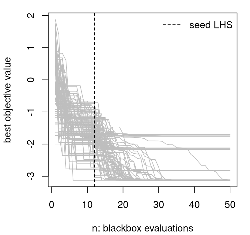
FIGURE 7.4: Multiple BOV progress paths following Figure 7.3 under random reinitialization.
Clearly this is not a global optimization tool. It looks like there are three or four local optima, or at least the optimizer is being pulled toward three or four domains of attraction. Before commenting further, it’ll be helpful to have something to compare to.
7.1.2 A classical comparator
How about our favorite optimization library: optim using "L-BFGS-B"? Working optim in as a comparator requires a slight tweak.
Code below modifies our objective function to help keep track of the full set of y-values gathered over optimization iterations, as these are not saved by optim in a way that’s useful for backing out a progress meter (e.g., prog) for comparison. (The optim method works just fine, but it was not designed with my illustrative purpose in mind. It wants to iterate to convergence and give the final result rather than bother you with the details of each evaluation. A trace argument prints partial evaluation information to the screen, but doesn’t return those values for later use.) So the code below updates a y object stored in the calling environment.
Below is the same for loop we did for EY-based surrogate-assisted optimization, but with a direct optim instead. A single random coordinate is used to initialize search, which means that optim enjoys ninit - 1 extra decision-based acquisitions compared to the surrogate method. (No handicap is applied. All expensive function evaluations count equally.) Although optim may utilize more than fifty iterations, our extraction of prog implements a cap of fifty.
prog.optim <- matrix(NA, nrow=reps, ncol=end)
for(r in 1:reps) {
  y <- c()
  os <- optim(runif(2), fprime, lower=0, upper=1, method="L-BFGS-B")
  prog.optim[r,] <- bov(y, end)
}
How does optim compare to surrogate-assisted optimization with EY? Figure 7.5 shows that surrogates are much better on a fixed budget. New prog measures for optim are shown in red.
matplot(t(prog.optim), type="l", col="red", lty=1,
  xlab="n: blackbox evaluations", ylab="best objective value")
matlines(t(prog), type="l", col="gray", lty=1)
legend("topright", c("EY", "optim"), col=c("gray", "red"), lty=1, bty="n")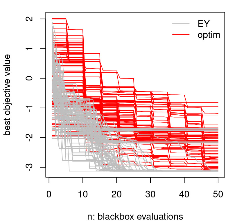
FIGURE 7.5: Augmenting Figure 7.4 to include a "L-BFGS-B" comparator under random restarts.
What makes EY so much better; or optim so much worse? Several things. First, "L-BFGS-B" spends precious blackbox evaluations on approximating derivatives. That explains the regular plateaus every five or so iterations. Each step spends roughly \(2m\) calls to \(f\) on calculating a tangent plane, alongside one further call at each newly chosen location, which is often just a short distance away. By comparison, surrogates provide a sense of derivative for “free”, not just locally but everywhere. The curious reader may wish to try method="Nelder-Mead" instead (Nelder and Mead 1965), which is the default in optim. Nelder-Mead doesn’t support search bounds, so the objective must be modified slightly to prevent search wandering well outside our domain of interest. Nelder-Mead doesn’t approximate derivatives, so its progress is a little “smoother” and also a little faster on this 2d problem (when constrained to the box), but is ultimately not as good as the surrogate method. I find that "L-BFGS-B" is more robust, especially in higher dimension, and I like that you can specify a bounding box.
Second, whereas optim, using "L-BFGS-B" or "Nelder-Mead", emphasizes local refinements – leveraging some limited memory, which is like using a model of sorts but not a statistical one – surrogates hold potential for large steps because their view of the response surface is more broad. On occasion, that helps EY escape from local minima, which is more likely in early rather than later iterations.
By and large, surrogate-assisted optimization with EY is still a local affair. Its advantages stem primarily from an enhanced sense of perspective. It exploits, by moving to the next best spot from where it left off, descending with its own optim subroutine on \(\mu_n(x)\). As implemented, it doesn’t explore places that cannot easily be reached from the current best value. It could help to initialize optim subroutines elsewhere, but the success of such variations is highly problem dependent. Sometimes it helps a little, sometimes it hurts.
What’s missing is some way to balance exploration and exploitation. By the way, notice that we’re not actually doing statistics, because at no point is uncertainty being taken into account. Only predictive means are used; predictive variance doesn’t factor in. One way to incorporate uncertainty is through the lower confidence bound (LCB) heuristic (Srinivas et al. 2009). LCB is a simple linear combination between mean and standard deviation:
\[\begin{equation} \alpha_{\mathrm{LCB}}(x) = - \mu_n(x) + \beta_n \sigma_n(x), \quad \mbox{ and } \quad x_{n+1} = \mathrm{argmax}_x \; \alpha_{\mathrm{LCB}}(x). \tag{7.1} \end{equation}\]
LCB introduces a sequence of tuning parameters \(\beta_n\), targeting a balance between exploration and exploitation as iterations of optimization progress. Larger \(\beta_n\) lead to more conservative searches, until in the limit \(\mu_n(x)\) is ignored and acquisitions reduce to ALM (§6.2.1). A family of optimal choices \(\hat{\beta}_n\) may be derived by minimizing regret in a multi-armed bandit setting, however in practice such theoretically automatic selections remain unwieldy for practitioners.
There’s a twist on EY, called Thompson sampling (Thompson 1933), that gracefully incorporates predictive uncertainty. Rather than optimize the predictive mean directly, take a draw from the (full covariance) posterior predictive distribution (5.3), and optimize that instead. Each iteration of search would involve a different, independent surrogate function draw. Therefore, a collection of many optimization steps would feel the effect of a sense of relative uncertainty through a diversity of such draws. Sparsely sampled parts of the input space could see large swings in surrogate optima, which would lead to exploratory behavior. No setting of tuning parameters required.
There are several disadvantages to Thompson sampling however. One is that it’s a stochastic optimization. Each iteration of optimization is based on an inherently random process. Another is that you must commit to a predictive grid in advance, in order to draw from posterior predictive equations, which rules out (continuous) library-based optimization in the inner loop, say by "L-BFGS-B". Actually it’s possible to get around a predictive grid with a substantially more elaborate implementation involving iterative applications of MVN conditionals (5.1). But there’s a better, easier, and more deterministic way to accomplish the same feat by deliberately acknowledging a role for predictive variability in acquisition criteria.
7.2 Expected improvement
In the mid 1990s, Matthias Schonlau (1997) was working on his dissertation, which basically revisited Mockus’ Bayesian optimization idea from a GP and computer experiments perspective. He came up with a heuristic called expected improvement (EI), which is the basis of the so-called efficient global optimization (EGO) algorithm. This distinction is subtle: one is the sequential design criterion (EI), and the other is its repeated application toward minimizing a blackbox function (EGO). In the literature, you’ll see the overall method referred to by both names/acronyms.
Schonlau’s key insight was that predictive uncertainty is underutilized by surrogate frameworks for optimization, which is especially a shame when GPs are involved because they provide such a beautiful predictive variance function. The basic tenets, however, are not limited to GP surrogates. The key is to link prediction to potential for optimization via a measure of improvement. Let \(f_{\min}^n = \min \{y_1, \dots, y_n\}\) be the smallest, best blackbox objective evaluation obtained so far, i.e., the BOV quantity we tracked with prog in our earlier illustrations. Schonlau defined potential for improvement over \(f_{\min}^n\) at an input location \(x\) as
\[ I(x) = \max\{0, f^{\mathrm{min}}_n - Y(x)\}. \]
\(I(x)\) is a random variable. It measures the amount by which a response \(Y(x)\) could be below the BOV obtained so far. Here \(Y(x)\) is shorthand for \(Y(x) \mid D_n\), the predictive distribution obtained from a fitted model. If \(Y(x) \mid D_n\) has nonzero probability of taking on any value on the real line, as it does under a Gaussian predictive distribution, then \(I(x)\) has nonzero probability of being positive for any \(x\).
Now there are lots of things you could imagine doing with \(I(x)\). (Something must be done because in its raw form, as a random variable, it’s of little practical value.) One option is to convert it into a probability. The probability of improvement (PI) criterion is \(\mathrm{PI}(x) = P(I(x) > 0 \mid D_n)\), which is equivalent to \(P(Y(x) < f_{\min}^n \mid D_n)\). Maximizing PI is sensible, but could result in very small steps. The most probable input \(x^\star = \max_x \mathrm{PI}(x)\) may not hold the greatest potential for large improvement, which is important when considering the tacit goal of minimizing the number of expensive blackbox evaluations. Instead, maximizing expected improvement (EI), \(\mathrm{EI}(x) = \mathbb{E}\{I(x) \mid D_n \}\), more squarely targets potential for large improvement.
The easiest way to calculate PI or EI, where “easy” means agnostic to the form of \(Y(x) \mid D_n\), is through MC approximation. Draw \(y^{(t)} \sim Y(x) \mid D_n\), for \(t=1,\dots, T\), from their posterior predictive distribution, and average
\[ \begin{aligned} \mathrm{PI}(x) &\approx \frac{1}{T} \sum_{t=1}^T \mathbb{I}_{\{y^{(t)} > 0\}} & & \mbox{or} & \mathrm{EI}(x) &\approx \frac{1}{T} \sum_{t=1}^T \max \{0, f^n_{\min} - y^{(t)} \}. \end{aligned} \]
In the limit as \(T \rightarrow \infty\) these approximations become exact. This approach works no matter what the distribution of \(Y(x)\) is, so long as you can simulate from it. With fully Bayesian response surface methods leveraging Markov chain Monte Carlo (MCMC) posterior sampling, say, such approximation may represent the only viable option.
However if \(Y(x) \mid D_n\) is Gaussian, as it’s under the predictive equations of a GP surrogate conditional on a particular set of hyperparameters, both have a convenient closed form. PI involves a standard Gaussian CDF (\(\Phi\)) evaluation, as readily calculated with built-in functions in R.
\[\begin{equation} \mathrm{PI}(x) = \Phi\left(\frac{f^n_{\min} - \mu_n(x)}{\sigma_n(x)}\right) \tag{7.2} \end{equation}\]
Transparent in the formula above is that both predictive mean and uncertainty factor into the calculation.
Deriving EI takes a little more work, but nothing an A+ student of calculus couldn’t do using substitution and integration by parts. Details are in an appendix of Schonlau’s thesis. I shall simply quote the final result here.
\[\begin{equation} \mathrm{EI}(x) = (f^n_{\min} - \mu_n(x))\,\Phi\!\left( \frac{f^n_{\min} - \mu_n(x)}{\sigma_n(x)}\right) + \sigma_n(x)\, \phi\!\left( \frac{f^n_{\min} - \mu_n(x)}{\sigma_n(x)}\right), \tag{7.3} \end{equation}\]
where \(\phi\) is the standard Gaussian PDF. Notice how EI contains PI as a component in a larger expression. “One half” of EI is PI multiplied (or weighted) by the amount by which the predictive mean is below \(f^n_{\min}\). The other “half” is predictive variance weighted by a Gaussian density evaluation. In this way, maximizing EI organically and transparently balances competing goals of exploitation (\(\mu_n(x)\) below \(f_{\min}^n\)) and exploration (large predictive uncertainty \(\sigma_n(x)\)).
In what follows the discussion drops PI and focuses exclusively on EI. An exercise in §7.4 encourages the curious reader to rework examples below by swapping in a simple PI implementation, in addition to other alternatives.
7.2.1 Classic EI illustration
As a first illustration of EI, code chunks below recreate an example and visuals presented in the first published/journal manuscript describing EI/EGO (Jones, Schonlau, and Welch 1998). I like to introduce Schonlau’s thesis first to give him proper credit, whereas the Journal of Global Optimization article linked in the previous sentence is often cited as Jones, et al. (1998). Consider data \(D_n = (X_n, Y_n)\) hand-coded in R below, which was taken by eyeball from Figure 10 in that paper, and re-centered to have a mean near zero. Observe the deliberate gap in the input space between fourth and fifth inputs, scanning from the left.
Code below initializes a GP fit on these data with hyperparameterization chosen to match that figure, again by eyeball. (It’s such a great example from a pedagogical perspective, I didn’t want to blow it. We’ll do a more dynamic and novel illustration shortly.) Predictions may then be obtained on a dense grid in the input space.
gpi <- newGP(matrix(x, ncol=1), y, d=10, g=1e-8)
xx <- seq(0, 13, length=1000)
p <- predGP(gpi, matrix(xx, ncol=1), lite=TRUE)
Ok, we have everything we need to calculate EI (7.3). R code below evaluates that equation using predictive quantities stored in p after calculating \(f^n_{\min}\) from the small initial set of y values.
m <- which.min(y)
fmin <- y[m]
d <- fmin - p$mean
s <- sqrt(p$s2)
dn <- d/s
ei <- d*pnorm(dn) + s*dnorm(dn)
The left panel in Figure 7.6 shows the predictive surface in terms of mean and approximate 95% error-bars. The predictive mean clearly indicates potential for a solution in the left half of the input space. Our simple surrogate-assisted EY optimizer (§7.1.2) would exploit that low mean and acquire the next point there. However, error-bars suggest great potential for minima in the right half of the input space. Although means are high there, error-bars fall well below the current best value \(f^n_{\min}\), suggesting exploration might be warranted. EI, shown in the right panel of the figure, synthesizes this information to strike a balance between exploration and exploitation.
par(mfrow=c(1,2))
plot(x, y, pch=19, xlim=c(0,13), ylim=c(-4,9), main="predictive surface")
lines(xx, p$mean)
lines(xx, p$mean + 2*sqrt(p$s2), col=2, lty=2)
lines(xx, p$mean - 2*sqrt(p$s2), col=2, lty=2)
abline(h=fmin, col=3, lty=3)
legend("topleft", c("mean", "95% PI", "fmin"), lty=1:3,
  col=1:3, bty="n")
plot(xx, ei, type="l", col="blue", main="EI", xlab="x", ylim=c(0,0.15))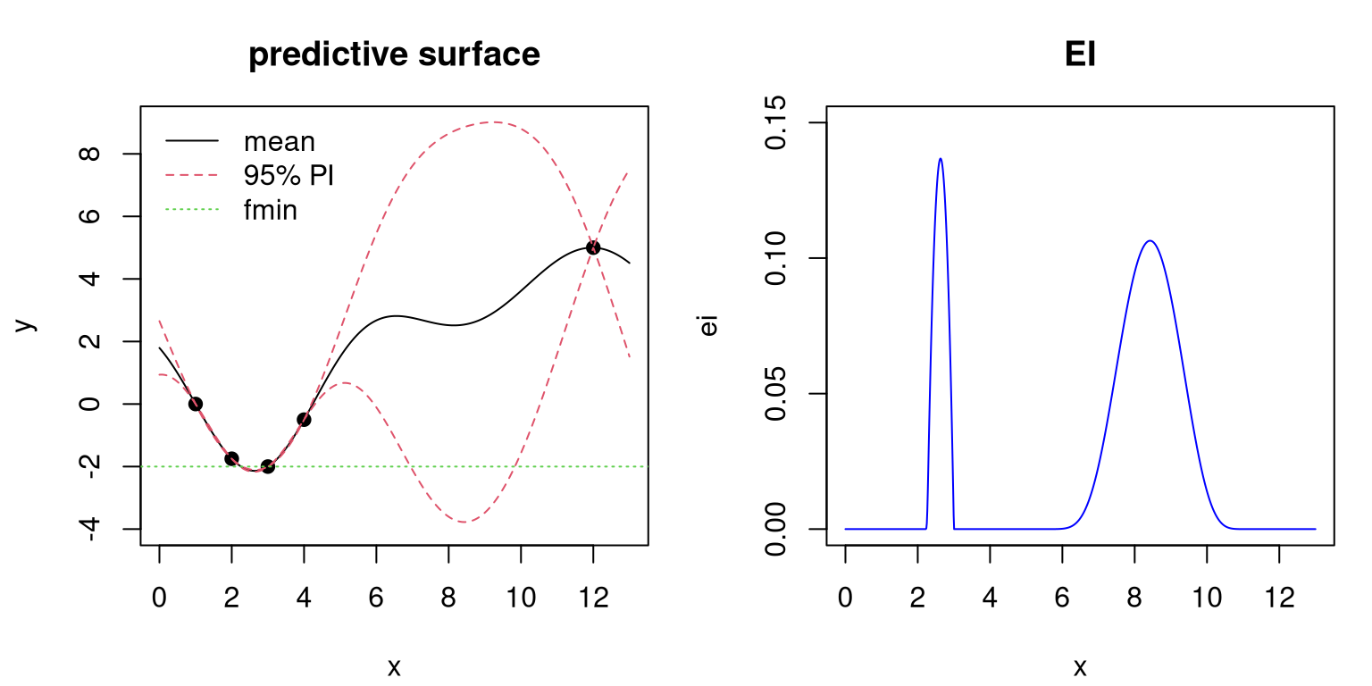
FIGURE 7.6: Classic EI illustration showing predictive surface (left) and corresponding EI surface (right).
That synthesis creates a multimodal EI surface. It’s a close call between the left and right options in the input space. Outside of those regions EI is essentially zero, although theoretically positive. The left mode is higher but narrower. Maximizing EI results in choosing the input for the next blackbox evaluation, \(x_{n+1}\), somewhere between 2 and 3. Options other than maximization, towards perhaps a better accounting for breadth of expected improvement, are discussed in §7.2.3. R code below makes a more precise selection and incorporates the new pair \((x_{n+1}, y_{n+1})\).
Notice that the predictive mean is being used for \(y_{n+1}\) in lieu of a “real” evaluation. For a clean illustration we’re supposing that our predictive mean was accurate, and that therefore we have a new global optima. A more realistic example follows soon. Code below updates the GP fit based on the new acquisition and re-evaluates predictive equations on our grid.
updateGP(gpi, matrix(xx[mm], ncol=1), p$mean[mm])
p <- predGP(gpi, matrix(xx, ncol=1), lite=TRUE)
deleteGP(gpi)
Cutting-and-pasting from above, next convert those predictions into EIs based on new \(f^n_{\min}\).
m <- which.min(y)
fmin <- y[m]
d <- fmin - p$mean
s <- sqrt(p$s2)
dn <- d/s
ei <- d*pnorm(dn) + s*dnorm(dn)
Updated predictive surface (left) and EI criterion (right) are provided in Figure 7.7.
par(mfrow=c(1,2))
plot(x, y, pch=19, xlim=c(0,13), ylim=c(-4,9), main="predictive surface")
lines(xx, p$mean)
lines(xx, p$mean + 2*sqrt(p$s2), col=2, lty=2)
lines(xx, p$mean - 2*sqrt(p$s2), col=2, lty=2)
abline(h=fmin, col=3, lty=3)
legend("topleft", c("mean", "95% PI", "fmin"), lty=1:3,
  col=1:3, bty="n")
plot(xx, ei, type="l", col="blue", main="EI", xlab="x", ylim=c(0,0.15))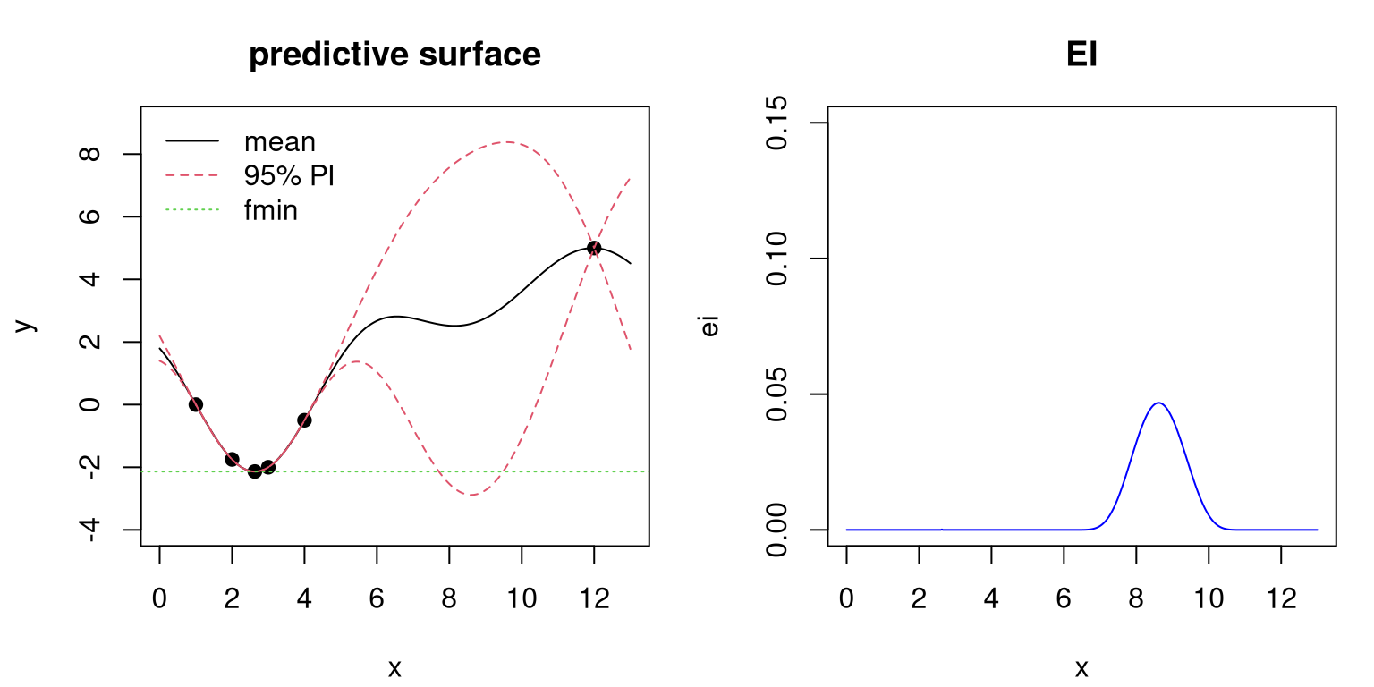
FIGURE 7.7: Predictive surface (left) and EI (right) after the first acquisition; see Figure 7.6.
There are several things to notice from the plots in the figure. Perhaps the most striking feature lies in the updated EI surface, which now contains just one bump. Elsewhere, EI is essentially zero. Choosing max EI will result in exploring the high variance region. The plot is careful to keep the same \(y\)-axis compared to Figure 7.6 in order to make transparent that EI tends to decrease as data are added. It need not always decrease, especially when hyperparameters are re-estimated when new data arrive. Since \(\hat{\tau}^2\) is analytic, laGP-based subroutines always keep this hyperparameter up to date. The implementation above doesn’t update lengthscale and nugget hyperparameters, but it could. Comparing left panels between Figures 7.6 and 7.7, notice that predictive variability has been reduced globally even though a point was added in an already densely-sampled area. Data affect GP fits globally under this stationary, default specification, although influence does diminish exponentially as gaps between training and testing locations grow in the input space.
We’re at the limits of this illustration because it doesn’t really involve a function \(f\), but rather some data on evaluations gleaned by eyeball from a figure in a research paper. A more interactive demo is provided as gp_ei_sin.R in supplementary material on the book web page. The demo extends our basic sinusoid example from §5.1.1, but is quite similar in flavor to the illustration above. Specifically, it combines an EI function from the plgp package (Gramacy 2014) with GP fitting from laGP (Gramacy and Sun 2018) – somewhat of a hodgepodge but it keeps the code short and sweet. For enhanced transparency on our running Goldstein–Price example (§7.1.1), we’ll code up our own EI function here, basically cut-and-paste from above, for use with laGP below.
EI <- function(gpi, x, fmin, pred=predGPsep)
 {
  if(is.null(nrow(x))) x <- matrix(x, nrow=1)
  p <- pred(gpi, x, lite=TRUE)
  d <- fmin - p$mean
  sigma <- sqrt(p$s2)
  dn <- d/sigma
  ei <- d*pnorm(dn) + sigma*dnorm(dn)
  return(ei)
 }
Observe how this implementation combines prediction with EI calculation. That’s a little inefficient in situations where we wish to record both predictive and EI quantities, as we did in the example above, especially when evaluating on a dense grid. Rather, it’s designed with implementation in Step 3 of Algorithm 6.1 in mind. The final argument, pred, enhances flexibility in specification of fitted model and associated prediction routine.
7.2.2 EI on our running example
To set up EI as an objective for minimization, the function below acts as a wrapper around - EI.
We’ve seen that EI can be multimodal, but it’s not pathologically so like ALM and, to a lesser extent, ALC. ALM/C inherit multimodality from the sausage-shaped GP predictive distribution. Although EI is composed of a measure of predictive uncertainty, its hybrid nature with the predictive mean has a calming effect. Consequently, EI is only high when both mean is low and variance is high, each contributing to potential for low function realization. The number of modes in EI may fluctuate throughout acquisition iterations, but in the long run should resemble the number of troughs in \(f\), assuming minimization. By contrast, the number of ALM/C modes would increase with \(n\). Like with ALM/C, a multi-start scheme for EI searches is sensible, but need not include \(\mathcal{O}(n)\) locations and these need not be as carefully placed, e.g., at the widest parts of the sausages. A fixed number, perhaps composed of the input location of the BOV (that corresponding to \(f^n_{\min}\), where we know the function is low) and a few other points spread around the input space, is often sufficient for decent performance. If not for numerical issues that sometimes arise when EI evaluations are numerically zero for large swaths of inputs, having just two multi-start locations (one at \(f_{\min}^n\) and one elsewhere) often suffices. Working with \(\log \mathrm{EI}(x)\) sometimes helps in such situations, but I won’t bother in our implementation here.
With those considerations in mind, the function below completes our solution to Algorithm 6.1, specifying \(J(x)\) in Step 3 for EI-based optimization. EI.search is similar in flavor to xnp1.search from §6.2.1, but tailored to EI and the multi-start scheme described above.
eps <- sqrt(.Machine$double.eps) ## used lots below

EI.search <- function(X, y, gpi, pred=predGPsep, multi.start=5, tol=eps)
 {
  m <- which.min(y)
  fmin <- y[m]
  start <- matrix(X[m,], nrow=1)
  if(multi.start > 1)
    start <- rbind(start, randomLHS(multi.start - 1, ncol(X)))
  xnew <- matrix(NA, nrow=nrow(start), ncol=ncol(X)+1)
  for(i in 1:nrow(start)) {
    if(EI(gpi, start[i,], fmin) <= tol) { out <- list(value=-Inf); next }
    out <- optim(start[i,], obj.EI, method="L-BFGS-B",
      lower=0, upper=1, gpi=gpi, pred=pred, fmin=fmin)
    xnew[i,] <- c(out$par, -out$value)
  }
  solns <- data.frame(cbind(start, xnew))
  names(solns) <- c("s1", "s2", "x1", "x2", "val")
  solns <- solns[solns$val > tol,]
  return(solns)
}
Although a degree of stochasticity is being injected through the multi-start scheme, this is simply to help the inner loop (maximizing EI), where evaluations are cheap. From the perspective of the outer loop – iterations of sequential design, with details coming momentarily – the intention is still to perform a deliberate and deterministic search. Actually more multi-start locations translate into more careful acquisitions \(x_{n+1}\) and subsequent expensive blackbox evaluation. The data.frame returned on output has one row for each multi-start location, although rows yielding effectively zero EI are culled. Multi-start locations whose first EI evaluation is effectively zero are immediately aborted. There are many further ways to “robustify” EI.search, but it’s surprising how well things work without much fuss. For example, Jones, Schonlau, and Welch (1998) suggested branch and bound search rather than multi-start derivative-based numerical optimization (optim in our implementation above). Providing gradients to optim can help too. But the improvements that those enhancements offer are at best slight in my experience.
All right, let’s initialize an EI-based optimization – same as for the two earlier comparators.
X <- randomLHS(ninit, 2)
y <- f(X)
gpi <- newGPsep(X, y, d=0.1, g=1e-6, dK=TRUE)
da <- darg(list(mle=TRUE, max=0.5), randomLHS(1000, 2))
Code below solves for the next input to try, extracting the best row from the output data.frame.
Before acting on that solution, Figure 7.8 summarizes the outcome of search with arrows indicating starting and ending locations of each multi-start EI optimization. Open circles mark the original/existing design. The red dot corresponds to the best row.
plot(X, xlab="x1", ylab="x2", xlim=c(0,1), ylim=c(0,1))
arrows(solns$s1, solns$s2, solns$x1, solns$x2, length=0.1)
points(solns$x1[m], solns$x2[m], col=2, pch=20)
FIGURE 7.8: First iteration of EI search on Goldstein–Price objective in the style of Figure 7.1.
One of the arrows originates from an open circle. This is the multi-start location corresponding to \(f_{\min}^n\). Up to four other arrows come from an LHS. If the total number of arrows is fewer than 5, the default multi.start in EI.search, that’s because some were initialized in numerically-zero EI locations, and consequently that search was voided at the outset. Usually two or more arrows appear, sometimes with distinct terminus indicating a multi-modal criterion.
Moving on now, code below incorporates the new data at the chosen input location (red dot) and updates the GP fit.
xnew <- as.matrix(solns[m,3:4])
X <- rbind(X, xnew)
y <- c(y, f(xnew))
updateGPsep(gpi, xnew, y[length(y)])
mle <- mleGPsep(gpi, param="d", tmin=da$min, tmax=da$max, ab=da$ab)
We’re ready for the next acquisition. Below the search is combined with a second GP update, after incorporating the newly selected data pair.
solns <- EI.search(X, y, gpi)
m <- which.max(solns$val)
maxei <- c(maxei, solns$val[m])
xnew <- as.matrix(solns[m,3:4])
X <- rbind(X, xnew)
y <- c(y, f(xnew))
updateGPsep(gpi, xnew, y[length(y)])
mle <- mleGPsep(gpi, param="d", tmin=da$min, tmax=da$max, ab=da$ab)
Figure 7.9 offers a visual, accompanied by a story that’s pretty similar to Figure 7.8.
plot(X, xlab="x1", ylab="x2", xlim=c(0,1), ylim=c(0,1))
arrows(solns$s1, solns$s2, solns$x1, solns$x2, length=0.1)
points(solns$x1[m], solns$x2[m], col=2, pch=20)
FIGURE 7.9: Second iteration of EI search after Figure 7.8.
You get the idea. Rather than continue with pedantic visuals, a for loop below repeats in this way until fifty samples of \(f\) have been collected. Hopefully one of them will offer a good solution to the optimization problem, an \(x^\star\) with a minimal objective value \(f(x^\star)\).
for(i in nrow(X):end) {
  solns <- EI.search(X, y, gpi)
  m <- which.max(solns$val)
  maxei <- c(maxei, solns$val[m])
  xnew <- as.matrix(solns[m,3:4])
  ynew <- f(xnew)
  X <- rbind(X, xnew)
  y <- c(y, ynew)
  updateGPsep(gpi, xnew, y[length(y)])
  mle <- mleGPsep(gpi, param="d", tmin=da$min, tmax=da$max, ab=da$ab)
}
deleteGPsep(gpi)
Notice that no stopping criteria are implemented in the loop. Our previous y-value-based criterion would not be appropriate here because progress isn’t measured by the value of the objective, but instead by potential for (expected) improvement. A relevant such quantity is recorded by maxei above. Still, y-progress is essential to drawing comparison to earlier results.
Figure 7.10 presents these two measures of progress side-by-side, with y on the left and maxei on the right.
par(mfrow=c(1,2))
plot(prog.ei, type="l", xlab="n: blackbox evaluations",
  ylab="EI best observed value")
abline(v=ninit, lty=2)
legend("topright", "seed LHS", lty=2)
plot(ninit:end, maxei, type="l",  xlim=c(1,end),
  xlab="n: blackbox evaluations", ylab="max EI")
abline(v=ninit, lty=2)
FIGURE 7.10: EI progress in terms of BOV (left) and maximal EI used for acquisition (right).
First, notice how BOV (on the left) is eventually in the vicinity of \(-3\), which is as good or better than anything we obtained in previous optimizations. Even in this random Rmarkdown build I can be pretty confident about that outcome for reasons that’ll become more apparent after we complete a full MC study, shortly. The right panel, showing EI progress, is usually spiky. As the GP learns about the response surface, globally, it revises which areas it believes are high variance, and which give low response values, culminating in dramatic shifts in potential for improvement. Eventually maximal EI settles down, but there’s no guarantee that it won’t “pop back up” if a GP update is surprised by an acquisition. Sometimes those “pops” are big, sometimes small. Therefore maxei is more useful as a visual confirmation of convergence than it is an operational one, e.g., one that can be engineered into a library function. Hence it’s common to run out an EI search to exhaust a budget of evaluations. The function below, designed to encapsulate code above for repeated calls in an MC setting, demands an end argument in lieu of more automatic convergence criteria.
optim.EI <- function(f, ninit, end)
 {
  ## initialization
  X <- randomLHS(ninit, 2)
  y <- f(X)
  gpi <- newGPsep(X, y, d=0.1, g=1e-6, dK=TRUE)
  da <- darg(list(mle=TRUE, max=0.5), randomLHS(1000, 2))
  mleGPsep(gpi, param="d", tmin=da$min, tmax=da$max, ab=da$ab)

  ## optimization loop of sequential acquisitions
  maxei <- c()
  for(i in (ninit+1):end) {
    solns <- EI.search(X, y, gpi)
    m <- which.max(solns$val)
    maxei <- c(maxei, solns$val[m])
    xnew <- as.matrix(solns[m,3:4])
    ynew <- f(xnew)
    updateGPsep(gpi, xnew, ynew)
    mleGPsep(gpi, param="d", tmin=da$min, tmax=da$max, ab=da$ab)
    X <- rbind(X, xnew)
    y <- c(y, ynew)
  }

  ## clean up and return
  deleteGPsep(gpi)
  return(list(X=X, y=y, maxei=maxei))
 }
This optim.EI function hard-codes a separable laGP-based GP formulation, but is easily modified for other settings or an isotropic analog. Using that function, let’s repeatedly solve the problem in this way (and track progress) with 100 random initializations, duplicating work similar to our EY and "L-BFGS-B" optimizations from §7.1.1–7.1.2.
reps <- 100
prog.ei <- matrix(NA, nrow=reps, ncol=end)
for(r in 1:reps) {
  os <- optim.EI(f, ninit, end)
  prog.ei[r,] <- bov(os$y)
}
Because showing three sets of 100 paths (300 total) would be a hot spaghetti mess, Figure 7.11 shows averages of those sets of 100 for our three comparators. Variability in those paths, which is mostly of interest for latter iterations/near the budget limit, is shown in a separate figure momentarily.
plot(colMeans(prog.ei), col=1, lwd=2, type="l",
  xlab="n: blackbox evaluations", ylab="average best objective value")
lines(colMeans(prog), col="gray", lwd=2)
lines(colMeans(prog.optim, na.rm=TRUE), col=2, lwd=2)
abline(v=ninit, lty=2)
legend("topright", c("optim", "EY", "EI", "seed LHS"),
  col=c(2, "gray", 1, 1), lwd=c(2,2,2,1), lty=c(1,1,1,2),
  bty="n")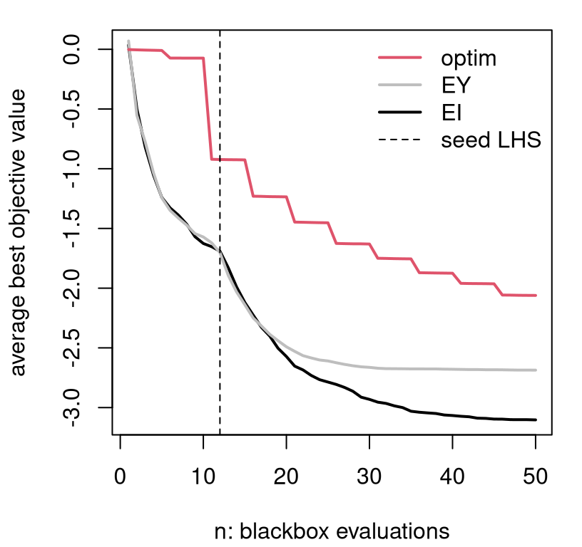
FIGURE 7.11: Average BOV progress for the three comparators entertained so far.
Although EI and EY perform similarly for the first few acquisitions after initialization, EI systematically outperforms in subsequent iterations. Whereas the classical surrogate-assisted EY heuristic gets stuck in inferior local optima, EI is better able to pop out and explore other alternatives. Both are clearly better than derivative-based methods like "L-BFGS-B", labeled as optim in Figure 7.11.
Figure 7.12 shows the diversity of solutions in the final, fiftieth iteration. Only in a small handful of 100 repeats does EI not find the global min after 50 iterations. Classical surrogate-assisted EY optimization fails to find the global optima about half of the time. Numerical "L-BFGS-B" optimization fails more than 75% of the time.
boxplot(prog.ei[,end], prog[,end], prog.optim[,end],
  names=c("EI", "EY", "optim"), border=c("black", "gray", "red"),
  xlab="comparator", ylab="best objective value")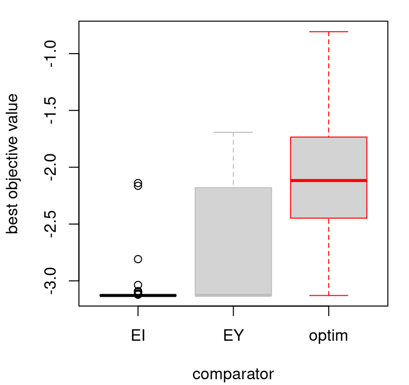
FIGURE 7.12: Boxplots summarizing the distribution of progress after the final acquisition.
All of the methods would benefit from more iterations, but only marginally unless random restarts are implemented for EY and optim comparators. Once those become stuck in a local minima they lack the ability to pop out on their own. EI, on the other hand, is in a certain sense guaranteed to become unstuck. Under certain regularity conditions, like that hyperparameters are fixed and known and the objective function isn’t completely at odds with typical GP modeling assumptions, the EGO algorithm (i.e., repeated EI searches) will eventually converge to a global optimum. As usual with such theorems, the devil is in the details of the assumptions hidden in those regularity conditions. When are those satisfied, or easily verified, in practice? The real sleight-of-hand here is in the notion of convergence, not in the assumptions. EGO really only converges in the sense that eventually it’ll explore everywhere. Since completely random search also has that property, the accomplishment isn’t all that extraordinary. But the fact that its searches do not look random, but work as well as random in the limit, offers some comfort.
Perhaps a more important, or more relevant, theoretical result is that you can show that each EI-based acquisition is best in a certain sense: selection of \(x_{n+1}\) by EI is optimal if \(n+1 = N\), where \(N\) is the total budget available for evaluations of \(f\). That is, EI is best if the next sample is the last one you plan to take, and your intention is to predict that \(\min_x \; \mu_{n+1}(x)\) is the global minimum. For a sample of technical details relating to convergence of EI-like methods, see Bull (2011). Another perspective views EI as a greedy heuristic approximating a fuller “look-ahead” scheme. In the burgeoning BO literature there are several alternative acquisition functions (Snoek, Larochelle, and Adams 2012), i.e., sequential design heuristics, with similar behavior and theory. Bect, Bachoc, and Ginsbourger (2016) provide a compelling framework for studying properties and variations of EGO/EI-like methods.
7.2.3 Conditional improvement
As an example of a scheme intimately related to EI, but which is in principle forward thinking and targets even broader scope, consider integrated expected conditional improvement [IECI; Gramacy and Lee (2011)]. IECI was designed for optimization under constraints, our next topic, and that transition motivates its discussion here amid myriad similarly motivated extensions (see, e.g., Snoek, Larochelle, and Adams 2012; Bect, Bachoc, and Ginsbourger 2016) and methods based on the knowledge gradient (KG, as described by J. Wu et al. 2017 and references therein). I make no claims that IECI is superior to these alternatives, or superior to EI or KG. Rather it’s a well-motivated choice I know well, adding some breadth to a discussion of acquisition functions for optimization, paired with convenient library support.
In essence, IECI is to EI what ALC is to ALM. Instead of optimizing directly, first integrate then optimize. Like with ALM to ALC, developing intermediate conditional criteria represents a crucial first step. Recall that ALC (§6.2.2) entails measuring variance at a reference location \(x\) after a new location \(x_{n+1}\) is added into the design. Then that gets integrated, or more approximately summed, over a wider set of \(x \in \mathcal{X}\).
Similarly, conditional improvement measures improvement at reference location \(x\), after another location \(x_{n+1}\) is added into the design.
\[ I(x \mid x_{n+1}) = \max \{0, f_{\min}^n - Y(x \mid x_{n+1}) \} \]
“Deduce” moments of the distribution of \(Y(x \mid x_{n+1}) \mid D_n\) as follows:
- \(\mathbb{E}\{Y(x \mid x_{n+1}) \mid D_n\} = \mu_n(x)\) since \(y_{n+1}\) has not come yet.
- \(\mathbb{V}\mathrm{ar}[Y(x \mid x_{n+1}) \mid D_n] = \sigma_{n+1}^2(x)\) follows the ordinary GP predictive equations (5.2) with \(X_{n+1} = (X_n^\top ; x_{n+1}^\top)^\top\) and hyperparameters learned at iteration \(n\). See Eq. (6.6) in §6.2.2. In practice, this quantity is most efficiently calculated with partitioned inverse equations (6.8), just like with ALC.
Integrating \(I(x \mid x_{n+1})\) with respect to \(Y(x \mid x_{n+1})\) yields the expected conditional improvement (ECI), i.e., the analog of EI for conditional improvement.
\[ \mathbb{E}\{I(x \mid x_{n+1}) \mid D_n \} = (f^n_{\min} - \mu_n(x))\,\Phi\!\left( \frac{f^n_{\min}\!-\!\mu_n(x)}{\sigma_{n+1}(x)}\right) + \sigma_{n+1}(x)\, \phi\!\left( \frac{f^n_{\min}\!-\!\mu_n(x)}{\sigma_{n+1}(x)}\right) \]
To obtain a function of \(x_{n+1}\) only, i.e., a criterion for sequential design, integrate over the reference set \(x \in \mathcal{X}\)
\[\begin{equation} \mathrm{IECI}(x_{n+1}) = - \int_{x\in\mathcal{X}} \mathbb{E}\{I(x \mid x_{n+1}) \mid D_n \} w(x) \; dx. \tag{7.4} \end{equation}\]
Such is the integrated expected conditional improvement (IECI), for some (possibly uniform) weights \(w(x)\). As with ALC, in practice that integral is approximated with a sum.
\[ \mathrm{IECI}(x_{n+1}) \approx - \frac{1}{T} \sum_{t=1}^T \mathbb{E}\{I(x^{(t)} \mid x_{n+1}) \} w(x^{(t)}) \quad \mbox{ where } \; x^{(t)} \sim p(\mathcal{X}), \; \mbox{ for } \; t=1,\dots,T, \]
and \(p(\mathcal{X})\) is a measure on the input space \(\mathcal{X}\) which may be uniform. Alternatively, one may combine weights and measures on \(\mathcal{X}\) into a single measure. For now, take both to be uniform in \([0,1]^m\).
The minus in IECI may look peculiar at first glance. Since \(I(x \mid x_{x+1})\) is, in some sense, a two-step measure, small values are preferred over larger ones. ALC similarly prefers smaller future variances. Instead of measuring improvement directly at \(x_{n+1}\), as EI does, IECI measures improvement in a roundabout way, assessing it at a reference point \(x\) under the hypothetical scenario that \(x_{n+1}\) is added into the design. If \(x\) still has high improvement after \(x_{n+1}\) has been added in, then \(x_{n+1}\) must not have had much influence on potential for improvement at \(x\). If \(x_{n+1}\) is influential at \(x\), then improvement at \(x\) should be small after \(x_{n+1}\) is added in, not large. Observe that the above argument makes tacit use of the assumption that \(\mathbb{E}\{I(x \mid x_{n+1})\} \leq \mathbb{E}\{I(x)\}\), for all \(x\in \mathcal{X}\), a kind of monotonicity condition.
Alternately, consider instead expected reduction in improvement (RI), analogous to reduction in variance from ALC.
\[ \mathrm{RI}(x_{n+1}) = \int_{x\in\mathcal{X}} (\mathbb{E}\{I(x) \mid D_n \} - \mathbb{E}\{I(x \mid x_{n+1}) \mid D_n \}) w(x) \; dx \]
Clearly we wish to maximize RI, to reduce the potential for future improvement as much as possible. And observe that \(\mathbb{E}\{I(x)\}\) doesn’t depend on \(x_{n+1}\), so it doesn’t contribute substantively to the criterion. What’s left is exactly IECI. In order for RI to be positive, the very same monotonicity condition must be satisfied. For ALC we don’t need to worry about monotonicity since, conditional on hyperparameters, future (\(n+1\)) variance is always lower than past (\(n\)) variance. It turns out that the definition of \(f_{\min}\) is crucial to determining whether or not monotonicity holds.
A drawing in Figure 7.13 illustrates how \(f_{\min}\) can influence ECI. Two choices of \(f_{\min}\) are entertained, drawn as horizontal lines. One uses only observed \(y\)-values, following exactly our definition above for \(f_{\min}\). The other takes \(f_{\min}\) from the extremum of the GP predictive mean, drawn as a solid parabolic curve: \(f_{\min} = \min_x \; \mu_n(x)\). EI is related to the area of the predictive density drawn as a solid line, plotted vertically and centered at \(\mu_n(x)\), which lies underneath the horizontal \(f_{\min}\) line(s). ECI is likewise derived from the area of the predictive density drawn as a dashed line lying below the horizontal \(f_{\min}\) line(s). This dashed density has the same mean/mode as the solid one, but is more sharply peaked by influence from \(x_{n+1}\).
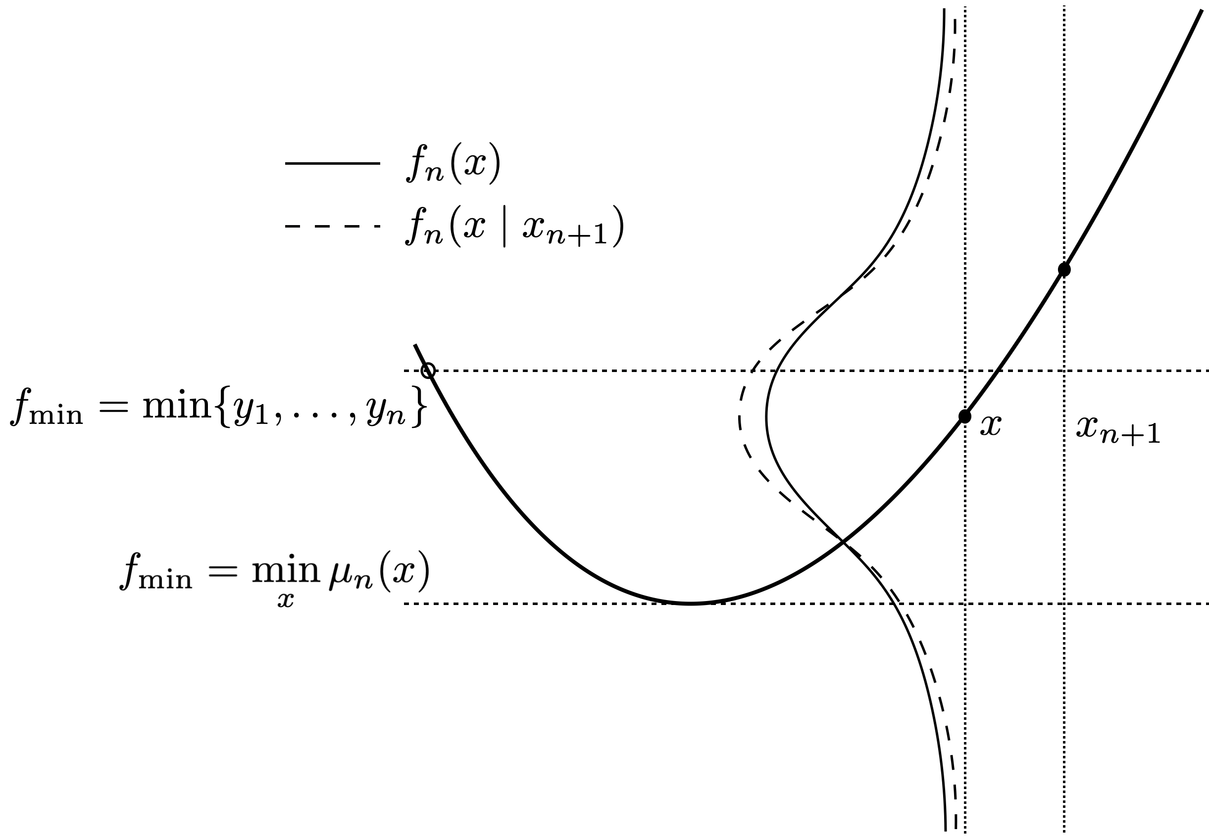
FIGURE 7.13: Cartoon illustrating how choice of \(f_{\min}\) affects ECI. Adapted from Gramacy and Lee (2011).
If we suppose that these densities, drawn as bell-shaped curves in the figure, are symmetric (as they are for GPs), then it’s clear that the relationship between ECI and EI depends upon \(f_{\min}\). As the dashed line is more peaked, the left-tail cumulative distributions have the property that \(F_n(f_{\min}\mid x_{n+1}) \geq F_n(f_{\min})\) for all \(f_{\min} \geq \mathbb{E}\{Y(x \mid x_{n+1})\} = \mathbb{E}\{Y(x)\}\). Since \(f_{\min} = \min \{y_1,\dots, y_n\}\) is one such example, we could observe \(\mathbb{E}\{I(x \mid x_{n+1})\} \geq \mathbb{E}\{I(x)\}\), violating the monotonicity condition. Only \(f_{\min} = \min_x \mu_n(x)\) guarantees that ECI represents a reduction compared to EI. That said, in practice the choice of \(f_{\min}\) matters little. But while we’re on the topic of what constitutes improvement – i.e., improvement upon what? – let’s take a short segue and talk about noisy blackbox objectives.
7.2.4 Noisy objectives
The BO literature over-accentuates discord between surrogate-assisted (EI or EY) optimization algorithms for deterministic and noisy blackboxes. The first paper on BO of stochastic simulations is by D. Huang et al. (2006). Since then the gulf between noisy and deterministic methods for BO has seemed to widen despite a surrogate modeling literature which has, if anything, downplayed the state(s) of affairs: Need a GP for noisy simulations? Just estimate a nugget. (With laGP, use jmleGP for isotropic formulations, or mleGPsep with param="both" for separable ones.) EI relies on the same underlying surrogates, so no additional changes are required there either, at least not to modeling aspects. Whenever noise is present, a modest degree of replication – especially in seed designs – can be helpful as a means of separating signal from noise. More details on that front are deferred to Chapter 10.
The notion of improvement requires a subtle change. Actually, nothing is wrong with the form of \(I(x)\), but how its components \(f_{\min}^n\) and \(Y(x) \mid D_n\) are defined. If there’s noise, then \(Y(x_i) \ne y_i\). Responses \(Y_1, \dots, Y_n\) at \(X_n\) are random variables. So \(f_{\min}^n\) is also a random variable. At face value, this substantially complicates matters. MC evaluations of EI, extending sampling of \(Y(x)\) to \(\min \{Y_1, \dots, Y_n\}\), may be the only faithful means of taking expectation over all random quantities. Fully analytic EI in such cases seems out of reach. Unfortunately, MC thwarts library-based optimization of EI. For example, simple optim methods wouldn’t work because the EI approximation would lack smoothness, except in the case of prohibitively large MC sampling efforts.
A common alternative is to use \(f_{\min} = \min_x \; \mu_n(x)\), exactly as suggested above to ensure the monotonicity condition, and proceed as usual. Picheny et al. (2013) call this the “plug-in” method. Plugging in deterministic \(\min_x \; \mu_n(x)\) for random \(f_{\min}\) works well despite under-accounting for a degree of uncertainty. It’s a refreshing coincidence that this choice of \(f_{\min}\) addresses both issues (monotonicity and noise), and that this choice makes sense intuitively. The quantity \(\min_x \; \mu_n(x)\) is our model’s best guess about the global function minimum, and \(\min_x \; \mu_{n+1}(x)\) is the one we intend to report when measuring progress. It stands to reason, then, that that value is sensible as a means of assessing potential to improve upon said predictions in subsequent acquisition iterations.
A second consideration for noisy cases involves the distribution of \(Y(x) \mid D_n\), via \(\mu_n(x)\) and \(\sigma_n^2(x)\) from the GP predictive equations (5.2). In the deterministic case, and when GP modeling without a nugget, \(\sigma_n^2(x) \rightarrow 0\) for all \(x\) as \(n \rightarrow \infty\). Here we’re assuming that \(X_n\) becomes dense in the input space as \(n\rightarrow \infty\), as improvement-based heuristics essentially guarantee. With enough data there’s no predictive uncertainty, so there’s eventually no value to any location by improvement \(I(x)\), either through EI or IECI. This makes sense: if you sample everywhere you’ll know all of the optima in the study region, both global and local. But in the stochastic case, and when GP modeling with a non-zero nugget, \(\sigma_n^2(x) \nrightarrow 0\) as \(n \rightarrow \infty\). No matter how much data is collected, there will always be predictive uncertainty in \(Y(x) \mid D_n\), so there will always be nonzero improvement \(I(x)\), through EI, IECI or otherwise. Our algorithm will never converge.
A simple fix is to redefine improvement on the latent random field \(f(x)\), rather than directly on \(Y(x)\). See §5.3.2 for details. Eventually, with enough data, there’s no uncertainty about the function – no epistemic uncertainty – even though there would be some aleatoric uncertainty about its noisy measurements. What that means, operationally speaking, is that when calculating EI one should use a predictive standard deviation without a nugget, as opposed to the full version (5.2). Specifically, and at slight risk of redundancy (5.16), use
\[\begin{equation} \breve{\sigma}_n^2(x) = \hat{\tau}^2 (1 - C(x, X_n) K_n^{-1} C(x, X_n)^\top) \tag{7.5} \end{equation}\]
rather than the usual \(\sigma_n^2(x) = \hat{\tau}^2 (1 + \hat{g}_n - C(x, X_n) K_n^{-1} C(x, X_n)^\top)\) in EI acquisitions. IECI is similar via \(\breve{\tilde{\sigma}}_{n+1}^2(x)\). Recall that \(\hat{g}_n\) is still involved in \(K_n^{-1}\), so the nugget is still being “felt” by predictions. Crucially, \(\breve{\sigma}_n^2(x) \rightarrow 0\) as \(n \rightarrow \infty\) as long as the design eventually fills the space. Library functions predGP and predGPsep provide \(\breve{\sigma}_n^2(x)\), or its multivariate analog, when supplied with argument nonug=TRUE.
Finally, Thompson sampling, which was dismissed earlier in §7.1.2 as a stochastic optimization, is worth reconsidering in noisy contexts. Noisy evaluation of the blackbox introduces a degree of stochasticity which can’t be avoided. A little extra randomness in acquisition criteria doesn’t hurt much and can sometimes be advantageous, especially when ambiguity between signal and noise regimes is present. See exercises in §7.4 for a specific example. Hybrids of LCB with EI have been successful in noisy optimization contexts. For example, quantile EI [QEI; Picheny et al. (2013)] works well when noise level can be linked to simulation fidelity; more on this and similar methods when we get to optimizing heterskedastic processes in Chapter 10.3.4.
7.2.5 Illustrating conditional improvement and noise
Let’s illustrate both IECI and optimization of a noisy blackbox at the same time. Consider the following data, which is in 1d to ease visualization.
fsindn <- function(x)
 sin(x) - 2.55*dnorm(x,1.6,0.45)
X <- matrix(c(0, 0.3, 0.6, 0.8, 1.0, 1.2, 1.4, 1.6, 1.8, 2.0, 2.2, 2.5,
  2.8, 3.1, 3.4, 3.7, 4.4, 5.3, 5.7, 6.1, 6.5, 7), ncol=1)
y <- fsindn(X) + rnorm(length(X), sd=0.15)
This seed design deliberately omits one of the two local minima of fsindn, although it’s otherwise uniformly spaced in the domain of interest, \(\mathcal{X} = [0,7]\). The code below initializes a GP fit, and performs inference for scale, lengthscale and nugget hyperparameters.
Before calculating EI and IECI, let’s peek at the predictive distribution. Code below extracts predictive quantities for both \(Y(x)\) and latent \(f(x)\), i.e., using \(\sigma_n^2(x)\) or \(\breve{\sigma}^2_n(x)\) from Eq. (7.5), respectively.
XX <- matrix(seq(0, 7, length=201), ncol=1)
pY <- predGP(gpi, XX, lite=TRUE)
pf <- predGP(gpi, XX, lite=TRUE, nonug=TRUE)
Figure 7.14 shows the mean surface, which is the same under both predictors, and two sets of error-bars. Red-dashed lines correspond to the usual error-bars, based on the full distribution of \(Y(x) \mid D_n\), using \(\sigma_n^2(x)\) above. Green-dotted ones use \(\breve{\sigma}^2_n(x)\) instead.
plot(X, y, xlab="x", ylab="y", ylim=c(-1.6,0.6), xlim=c(0,7.5))
lines(XX, pY$mean)
lines(XX, pY$mean + 1.96*sqrt(pY$s2), col=2, lty=2)
lines(XX, pY$mean - 1.96*sqrt(pY$s2), col=2, lty=2)
lines(XX, pf$mean + 1.96*sqrt(pf$s2), col=3, lty=3)
lines(XX, pf$mean - 1.96*sqrt(pf$s2), col=3, lty=3)
legend("bottomright", c("Y-bars", "f-bars"), col=2:4, lty=2:3, bty="n")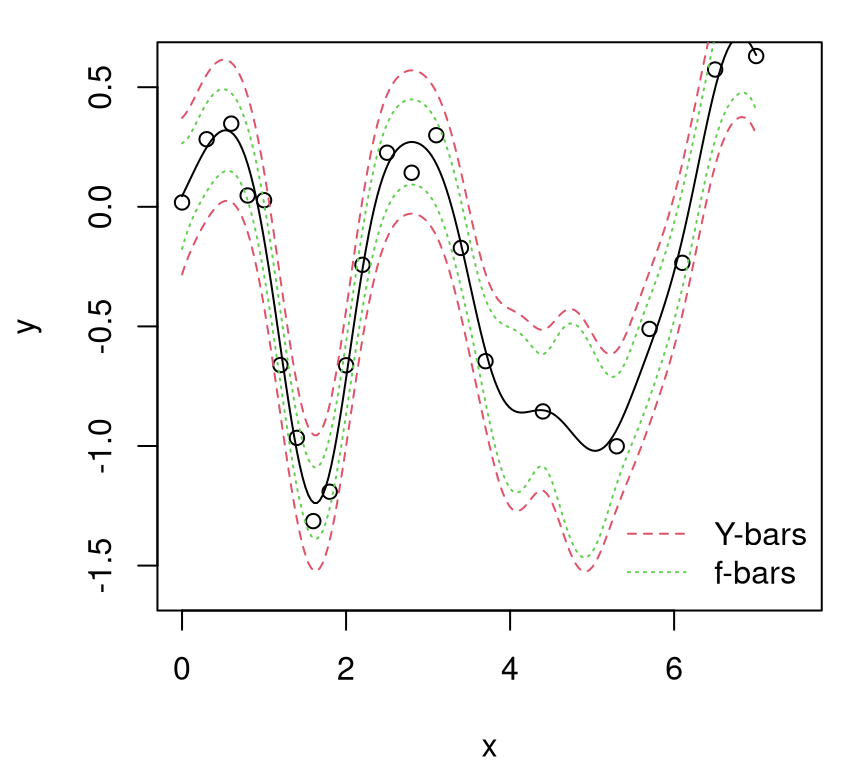
FIGURE 7.14: Comparing predictive quantiles under \(Y(x)\) and \(f(x)\).
Observe how “f-bars” quantiles are uniformly narrower than their “Y-bars” counterpart. With enough data \(D_n\), as \(n \rightarrow \infty\) and \(X_n\) filling the space, “f-bars” would collapse in on the mean surface, shown as the solid black line.
Now we’re ready to calculate EI and IECI under those two predictive distributions. EI with nonug=TRUE can be achieved by passing in a predictor pred with that option pre-set, e.g., by copying the function and modifying its default arguments (its formals). The ieciGP function provided by laGP has its own nonug argument. By default, ieciGP takes candidate locations, XX in the code below, identical to reference locations Xref, similar to alcGP.
fmin <- min(predGP(gpi, X, lite=TRUE)$mean)
ei <- EI(gpi, XX, fmin, pred=predGP)
ieci <- ieciGP(gpi, XX, fmin)
predGPnonug <- predGP
formals(predGPnonug)$nonug <- TRUE
ei.f <- EI(gpi, XX, fmin, pred=predGPnonug)
ieci.f <- ieciGP(gpi, XX, fmin, nonug=TRUE)
To ease visualization, it helps to normalize acquisition function evaluations so that they span the same range.
ei <- scale(ei, min(ei), max(ei) - min(ei))
ei.f <- scale(ei.f, min(ei.f), max(ei.f) - min(ei.f))
ieci <- scale(ieci, min(ieci), max(ieci) - min(ieci))
ieci.f <- scale(ieci.f, min(ieci.f), max(ieci.f) - min(ieci.f))
Figure 7.15 shows these four acquisition comparators. Solid lines are for EI, and dashed for IECI; the color scheme matches up with predictive surfaces above, where “-f” is the nonug=TRUE version, i.e., based on the latent random field \(f\). So that all are maximizable criteria, negative IECIs are plotted.
plot(XX, ei, type="l", ylim=c(0, 1), xlim=c(0,7.5), col=2, lty=1,
  xlab="x", ylab="improvements")
lines(XX, ei.f, col=3, lty=1)
points(X, rep(0, nrow(X)))
lines(XX, 1-ieci, col=2, lty=2)
lines(XX, 1-ieci.f, col=3, lty=2)
legend("topright", c("EI", "EI-f", "IECI", "IECI-f"), lty=c(1,1,2,2),
  col=c(2,3,2,3), bty="n")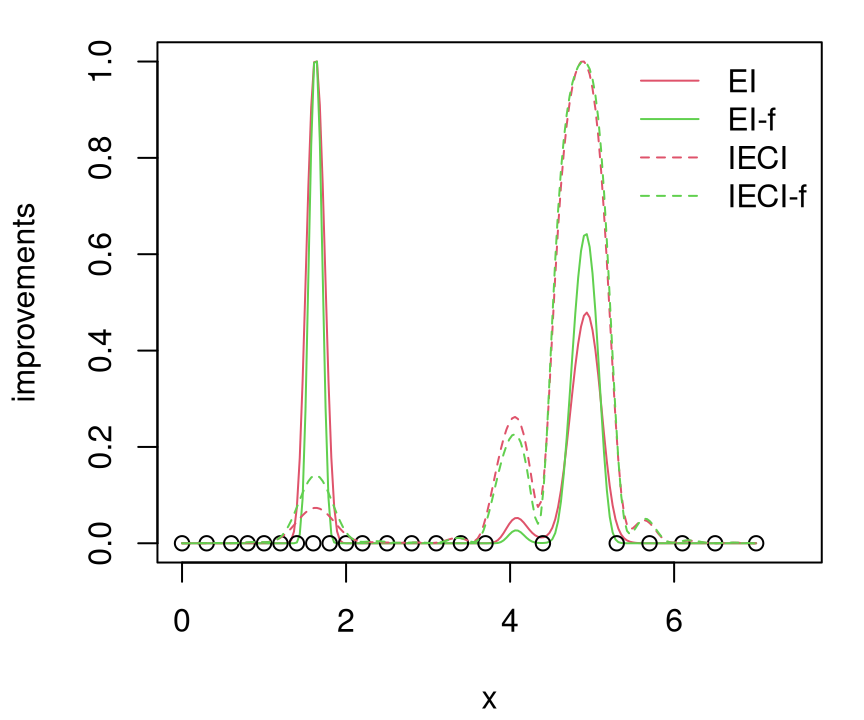
FIGURE 7.15: EI versus IECI in \(Y(x)\) and \(f(x)\) alternatives.
Since training data were randomly generated for this Rmarkdown build, it’s hard to pinpoint exactly the state of affairs illustrated in Figure 7.15. Usually EI prefers (in both variants) to choose \(x_{n+1}\) from the left half of the space, whereas IECI (both variants) weighs both minima more equally. Occasionally, however, EI prefers the right mode instead, and occasionally both prefer the left, all depending on the random data. Both represent local minima, but the one on the right experiences higher aggregate uncertainty due both to lower sampling and to a wider domain of attraction. The left minima has a narrow trough. As a more aggregate measure, IECI usually up-weights \(x_{n+1}\) from the right half, pooling together large ECI in a bigger geographical region, and consequently putting greater value on their potential to offer improvement globally in the input space.
Both EI and IECI cope with noise just fine. Variations with and without nugget are subtle, at least as exemplified by Figure 7.15. A careful inspection of the code behind that figure reveals that we didn’t actually minimize \(\mu_n(x)\) to choose \(f_{\min}^n\). Rather it was sufficient to use \(\min_i \mu_n(x_i)\), which is less work computationally because no auxiliary numerical optimization is required.
Rather than exhaust the reader with more for loops, say to incorporate IECI and noise into a bakeoff or to augment our running example (§7.1.1) on the (possibly noise-augmented) Goldstein–Price function, these are left to exercises in §7.4. IECI, while enjoying a certain conservative edge by “looking ahead”, rarely outperforms the simpler but more myopic ordinary EI in practice. This is perhaps in part because it’s challenging to engineer a test problem, like the one in our illustration above, exploiting just the scenario IECI was designed to hedge against. Both EI and IECI can be recast into the stepwise uncertainty reduction (SUR) framework (Bect, Bachoc, and Ginsbourger 2016) where one can show that they enjoy a supermartingale property, similar to a submodularity property common to many active learning techniques. But that doesn’t address the extent to which IECI’s limited degree of lookahead may or may not be of benefit, by comparison to EI say, along an arc of future iterations in the steps of a sequential design. Advantages or otherwise are problem dependent. In a context where blackbox objective functions \(f(x)\) almost never satisfy technical assumptions imposed by theory – the Goldstein–Price function isn’t a stationary GP – intuition may be the best guide to relative merits in practice.
Where IECI really shines is in a constrained optimization context, as this is what it was originally designed for – making for a nice segue into our next topic.
7.3 Optimization under constraints
To start off, we’ll keep it super simple and assume constraints are known, but that they take on non-trivial form. That is, not box/bound constraints (too easy), but something tracing out non-convex or even unconnected regions. Then we’ll move on to unknown, or blackbox constraints which require expensive evaluations to probe. First we’ll treat those as binary, valid or invalid, and then as real-valued. That distinction, binary or real-valued, impacts how constraints are modeled and how they fold into an effective sequential design criteria for optimization. Throughout, the goal is to find the best valid value (BVV) of the objective in the fewest number of blackbox evaluations. More details on the problem formulation(s) are provided below.
7.3.1 Known constraints
For now, assume constraints are known. Specifically, presume that we have access to a function, \(c(x): \mathcal{X} \rightarrow \{0,1\}\), returning zero (or equivalently a negative number) if the constraint is satisfied, or one (or a positive number) if the constraint is violated, and that we can evaluate it for “free”, i.e., as much as we want. Evaluation expense accrues on blackbox objective \(f(x)\) only.
The problem is given formally by the mathematical program
\[\begin{equation} x^\star = \mathrm{argmin}_{x \in \mathcal{\mathcal{X}}} \; f(x) \quad \mbox{ subject to } \quad c(x) \leq 0. \tag{7.6} \end{equation}\]
One simple surrogate-assisted solver entails extending EI to what’s called expected feasible improvement (EFI), which was described in a companion paper to the EI one by the same three authors, but with names of the first two authors swapped (Schonlau, Welch, and Jones 1998).
\[ \mbox{EFI}(x) = \mathbb{E}\{I(x)\} \mathbb{I}(c(x) \leq 0), \]
with \(I(x)\) using an \(f_{\min}^n\) defined over the valid region only. In deterministic settings, that means \(f_{\min}^n = \min_{i=1,\dots,n} \, \{y_i : c(x_i) \leq 0 \}\). When noise is present \(f_{\min}^n = \min_{x \in \mathcal{X}} \{ \mu_n(x) : c(x) \leq 0\}\). The former may be the empty set, in which case the latter is a good backup except in the pathological case that none of the study region \(\mathcal{X}\) is valid.
A verbal description of EFI might be: do EI but don’t bother evaluating, nor modeling, outside the valid region. Seems sensible: invalid evaluations can’t be solutions. We know in advance which inputs are in which set, valid or invalid, so don’t bother wasting precious blackbox evaluations that can’t improve upon the best solution so far.
Yet that may be an overly simplistic view. Mathematical programmers long ago found that approaching local solutions from outside of valid sets can sometimes be more effective than the other way around, especially if the valid region is comprised of disjoint or highly non-convex sets. One example is the augmented Lagrangian method, which we shall review in more detail in §7.3.4.
Surrogate modeling considerations also play a role here. Data acquisitions under GPs have a global effect on the updated predictive surface. Information from observations of the blackbox objective outside of the valid region might provide more insight into potential for improvement (inside the region) than any point inside the region could. Think of an invalid region sandwiched between two valid ones (see Figures 7.16–7.17) and how predictive uncertainty might look, and in particular its curvature, at the boundaries. One evaluation splitting the difference between the two boundaries may be nearly as effective as two right on each boundary. EFI would rule out that potential economy. Or, in situations where one really doesn’t want, or can’t perform an “invalid run”, but is still faced with a choice between high EI on either side of the invalid-region boundary, it might make sense to weigh potential for improvement by the amount of the valid region a potential acquisition would cover. That’s exactly what IECI was designed to do.
Adapting IECI to respect a constraint, but to still allow selection of evaluations “wherever they’re most effective”, is a matter of choosing indicator \(\mathbb{I}(c(x) \leq 0)\) as weight \(w(x)\):
\[ \mathrm{IECI}(x_{n+1}) = - \int_{x\in\mathcal{X}} \mathbb{E}\{I(x \mid x_{n+1})\} \mathbb{I}(c(x) \leq 0) \; dx \]
This downweights reference \(x\)-values not satisfying the constraint, and thus also \(x_{n+1}\)-values similarly, however it doesn’t preclude \(x_{n+1}\)-values from being chosen in the invalid region. Rather, the value of \(x_{n+1}\) is judged by its ability to impact improvement within the valid region. An alternative implementation which may be computationally more advantageous, especially when approximating the integral with a sum over a potentially dense collection Xref \(\subseteq \mathcal{X}\), is to exclude from Xref any input locations which don’t satisfy the constraint. More precisely,
\[ \mathrm{IECI}(x_{n+1}) \approx - \frac{1}{T} \sum_{t=1}^T \mathbb{E}\{I(x^{(t)} \mid x_{n+1}) \} \quad \mbox{ where } \; x^{(t)} \sim p_c(\mathcal{X}), \; \mbox{ for } \; t=1,\dots,T, \]
and \(p_c(\mathcal{X})\) is uniform on the valid set \(\{x\in \mathcal{X} : c(x) \leq 0\}\).
To illustrate, consider the same 1d data-generating mechanism as in §7.2.5 except with an invalid region \([2,4]\) sandwiched between two valid regions occupying the first and last third of the input space, respectively.
X <- matrix(c(0, 0.3, 0.6, 0.8, 1.0, 1.2, 1.4, 1.6, 1.8, 4.4, 5.3, 5.7,
  6.1, 6.5, 7), ncol=1)
y <- fsindn(X) + rnorm(length(X), sd=0.15)
No observations lie in the invalid region, yet. For dramatic effect in this illustration, it makes sense to hard-code a longer lengthscale when fitting the GP.
Readers are strongly advised to tinker with this (also with jmleGP) to see how it effects the results. Next, establish a dense grid in the input space \(\mathcal{X} \equiv\) XX and take evaluations of GP predictive equations thereupon.
Figure 7.16 shows the resulting predictive surface.
plot(X, y, xlab="x", ylab="y", ylim=c(-3.25, 0.7))
lines(XX, p$mean)
lines(XX, p$mean + 1.96*sqrt(p$s2), col=2, lty=2)
lines(XX, p$mean - 1.96*sqrt(p$s2), col=2, lty=2)![Predictive surface for a 1d problem with invalid region $[2,4]$ sandwiched between two valid ones.](surrogates_files/figure-html/sandwich-1.png)
FIGURE 7.16: Predictive surface for a 1d problem with invalid region \([2,4]\) sandwiched between two valid ones.
Because there are no evaluations in the middle third of the space, predictive uncertainty is very high there. Since the lengthscale is long, the posterior mean on functions favors a trough in that region, which translates into a promising solution to the constrained optimization problem – a valid global minimum. It seems quite likely that one of two local valid minima reside on either side of the invalid region.
First consider calculating EI for each XX location on the predictive grid, then normalizing to ease later visualization. In this illustration, only the nonug=TRUE option is shown, primarily to simplify visuals.
fmin <- min(predGP(gpi, X, lite=TRUE)$mean)
ei <- EI(gpi, XX, fmin, pred=predGPnonug)
ei <- scale(ei, min(ei), max(ei) - min(ei))
Ordinarily here, we’d have to be careful to calculate \(f_{\min}^n\) based only on valid input locations. However in this simple example all seed design X locations are valid. (And we know EFI won’t choose any invalid ones.) The code below extracts EIs for the valid region, effectively implementing EFI but in a way that’s handy for our visualization below.
To facilitate IECI calculation, the next code chunk establishes a set of reference locations Xref dense in \(\mathcal{X} \equiv\) XX, but similarly omitting invalid region \([2,4]\).
Using that pre-selected Xref in lieu of weights, laGP’s IECI subroutine may be evaluated for all of XX as follows.
ieci <- ieciGP(gpi, XX, fmin, Xref=Xref, nonug=TRUE)
ieci <- scale(ieci, min(ieci), max(ieci) - min(ieci))
Figure 7.17 compares EI/EFI and IECI in this known constraints setting. A solid-black line corresponds to EFI extracted from EI which is dashed within the invalid region.
plot(XX, ei, type="l", ylim=c(0, max(ei)), lty=2, xlab="x",
  ylab="normalized improvements")
lines(Xref[Xref < lc], eiref[Xref < lc])
lines(Xref[Xref > rc], eiref[Xref > rc])
points(X, rep(0, nrow(X)))
lines(XX, 1-ieci, col=2, lty=2)
legend("topright", c("EI", "IECI"), lty=1:2, col=1:2, bty="n")
abline(v=c(lc,rc), col="gray", lty=2)
text(lc,0,"]")
text(rc,0,"[")
text(seq(lc+.1, rc-.1, length=20), rep(0, 20), rep("/", 20))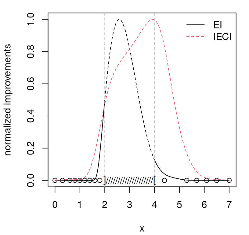
FIGURE 7.17: EFI and IECI surfaces for a simple 1d constrained optimization with invalid region sandwiched between two valid regions.
Notice how EI is maximized within the invalid region, but we won’t choose \(x_{n+1}\) there because its EFI is zero. Instead, EFI is maximized at the boundary of the invalid region, with nearly identical height on either side. IECI, by contrast, is maximized outside the valid region – at least in this random Rmarkdown instance – offering clear adjudication between the two local EFI modes. IECI prefers the right-hand mode, and not on the boundary with the invalid region but instead splitting the difference between boundary and design locations \(X_n\) already in hand. For my money, IECI’s is a better choice for \(x_{n+1}\).
In sequential application, over repeated acquisitions, admittedly EFI and IECI perform similarly. Which is better is highly problem specific, depending in particular on how complicated the valid region is, and how pathological interaction is between constraint boundary and blackbox objective. For many problems, IECI is likely overkill since it’s more computationally demanding, like ALC.
On the other hand, known constraint settings are specialized – you might even say highly peculiar. How often do you encounter a known constraint region that’s complicated in practice?
7.3.2 Blackbox binary constraints
Having a blackbox that simultaneously evaluates both objective and constraint at great computational expense is far more common. The mathematical program (7.6) is unchanged, but now constraints \(c(x)\) cannot be evaluated at will. Often blackbox constraint functions are vector-valued. In that case, the simple program (7.6) still applies, but \(c(x) \leq 0\) must be interpreted component-wise and valid re-defined to mean that all components satisfy the inequality simultaneously. Like for objective \(f(x)\), we’ll need a surrogate model for constraint \(c(x)\), and an appropriate model will depend upon the nature of the function(s). When binary, either \(c(x) \in \{0,1\}\) or \(c(x) \in \{0,1\}^m\) for multiple constraints, a classification model may be appropriate. When real-valued \(c(x) \in \mathbb{R}\) or \(c(x) \in \mathbb{R}^m\), a regression model is needed.
We can get as fancy or simple as we want with constraint models and fitting schemes. GPs are an obvious choice for real-valued cases, as we illustrate in §7.3.4. For now stick with binary constraints. GPs are an option for binary outputs too, e.g., through a logistic link (see, e.g., Chapter 3 of Rasmussen and Williams 2006), but there are simpler off-the-shelf classifiers that often work as well or better in practice. Details are forthcoming in our empirical work below. For now, the presentation is agnostic to choice of classifier. Let \(p^{(j)}_n(x)\) stand in for the predicted probability, from fitted surrogate model classifier(s), that input \(x\) satisfies the \(j^{\mathrm{th}}\) constraint, for \(j=1,\dots,m\).
Extending EFI to blackbox constraints is trivial. Simply replace the indicator (from the known constraint) with the surrogate’s predicted probability of satisfaction:
\[ \mbox{EFI}(x) = \mathbb{E}\{I(x)\} \prod_{j=1}^m p^{(j)}_n(x). \]
IECI is no different, except the product moves inside the integral.
\[ \mathrm{IECI}(x_{n+1}) = - \int_{x\in\mathcal{X}} \mathbb{E}\{I(x \mid x_{n+1})\} \prod_{j=1}^m p_n^{(j)}(x) \; dx \]
In both cases EI is being weighted by the joint probability of constraint satisfaction, assuming mutually independent constraint surrogates. Explicitly for IECI as in Eq. (7.4), take \(w(x) = \prod_{j=1}^m p_n^{(j)}(x)\).
To illustrate, revisit our earlier 1d known constraint problem fsindn from §7.2.5. This time imagine the constraint, which was invalid in \([2,4]\), as residing inside the blackbox. Expensive evaluations provide noisy \(Y(x) = f(x) + \varepsilon\) and deterministic \(c(x) \in \{0,1\}\), simultaneously. Model \(f\) with a GP, as before. In order to learn the constraint function from data, choose a simple yet flexible model from off the shelf: a random forest [RF; Breiman (2001)] via randomForest (Breiman et al. 2018) on CRAN.
Consider EFI first; returning to IECI shortly. A setup like this (GP/RF/EFI) was first entertained by H. Lee et al. (2011). The code below generates a small quasi-space-filling design to start out with, and evaluates the blackbox at those locations.
ninit <- 6
X <- matrix(c(1, 3, 4, 5, 6, 7))
y <- fsindn(X) + rnorm(length(X), sd=0.15)
const <- as.numeric(X > lc & X < rc)
Now fit surrogates. The block of code below targets GP fitting of the objective. With such a small amount of noisy data, it’s sensible to constrain inference a little to help the GP separate signal from noise. Recall our discussion in §6.2.1 on care in initialization with sequential design. Below the lengthscale is fixed, and the nugget estimated conditionally under a sensible prior. As more data are gathered, such precautions become less necessary.
gpi <- newGP(X, y, d=1, g=0.1*var(y), dK=TRUE)
ga <- garg(list(mle=TRUE, max=var(y)), y)
mle <- mleGP(gpi, param="g", tmin=eps, tmax=var(y), ab=ga$ab)
Next load randomForest and fit constraint evaluations, being careful to coerce them into factor form so that the library knows to fit a classification model rather than the default regression option for real-valued responses.
Below, \(f_{\min}\) is calculated by a smoothing over outputs predicted at valid input locations in \(X_n\). The number and location of samples in the seed design was chosen (based on oracle knowledge of the constraint) so that the set of valid locations is nonempty in order to simplify, somewhat, the exposition here. (In fact, a single invalid input is guaranteed.)
We now have all ingredients needed to evaluate EI and the probability of constraint satisfaction, globally in the input space over predictive grid XX.
pc <- predict(cfit, XX, type="prob")[,1]
ei <- EI(gpi, XX, fmin, pred=predGPnonug)
ei <- scale(ei, min(ei), max(ei) - min(ei))The EI surface, probability of satisfaction, and their product yielding EFI are shown together in Figure 7.18. Constraint evaluations are indicated as open circles. So that the parity of constraint evaluations matches probability of satisfaction, easing visualization, \(1-c_i\), \(i=1,\dots, n\) are plotted instead instead of raw \(c_i\).
plot(XX, ei, type="l", xlim=c(0,8), ylim=c(0,1), xlab="x", ylab="ei & pc")
lines(XX, pc, col=2, lty=2)
points(X, 1 - const, col=2)
lines(XX, ei*pc, lty=2)
legend("right", c("EI", "p(c<0)", "EFI"), col=c(1,2,1),
lty=c(1,2,2), bty="n")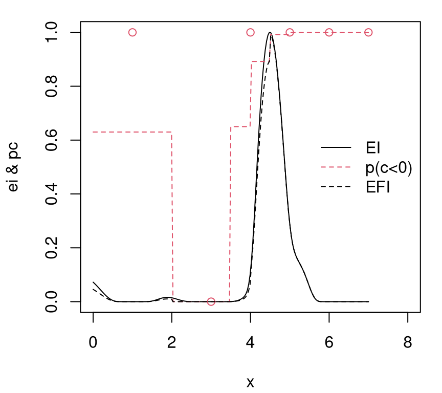
FIGURE 7.18: EI\((x)\) and \(p(c(x) < 0)\) combining to form EFI\((x)\). Open circles indicate \(1 - c_i\) to match parity with RF’s \(p(c_i < 0)\). EI and EFI are normalized.
Several interesting observations in the figure are worth remarking upon. Notice that \(p_n(x) \equiv\) p(c<0) is zero nearby the single input having violated the constraint (plotted as \(c_i = 0\), but actually measured as \(c_i = 1\)). This will cause EFI to evaluate to zero regardless of what EI is, but actually it’s essentially zero there anyways. Likewise, throughout the rest of the input space, EFI is a version of EI modulated slightly downwards, more so approaching the middle of the input space where the RF classifier is less sure about the transition from valid to invalid region. EFI inherits discontinuities from RF’s stepwise regime changes. The extent to which such discontinuities are detectable visually depends upon the Rmarkdown build.
After numerically maximizing EFI on the grid, code below acquires new \(x_{n+1}\), updating \(n \leftarrow n+1\) with a new random objective and deterministic constraint evaluation.
m <- which.max(ei*pc)
X <- rbind(X, XX[m,])
y <- c(y, fsindn(XX[m,]) + rnorm(1, sd=0.15))
const <- c(const, as.numeric(XX[m,] > lc && XX[m,] < rc))Next, update GP and RF fits to ready those surrogates for the next acquisition.
updateGP(gpi, X[nrow(X),,drop=FALSE], y[length(y)])
mle <- mleGP(gpi, param="g", tmin=eps, tmax=var(y), ab=ga$ab)
cfit <- randomForest(X, as.factor(const))In that subsequent iteration, \(f_{min}^n\) is recalculated based on the corpus of valid inputs obtained so far. Predictions under both models are evaluated at candidates \(\mathcal{X} \equiv\) XX, and EI’s are calculated, collecting all ingredients for EFI.
Xv <- X[const <= 0,,drop=FALSE]
fmin <- min(predGP(gpi, Xv, lite=TRUE)$mean)
pc <- predict(cfit, XX, type="prob")[,1]
ei <- EI(gpi, XX, fmin, pred=predGPnonug)
ei <- scale(ei, min(ei), max(ei) - min(ei))Updated EFI surface, and its requisite components are shown visually in Figure 7.19.
plot(XX, ei, type="l", xlim=c(0,8), ylim=c(0,1), xlab="x", ylab="ei & pc")
lines(XX, pc, col=2, lty=2)
points(X, 1 - const, col=2)
lines(XX, ei*pc, lty=2)
legend("right", c("EI", "p(c<0)", "EFI"), col=c(1,2,1),
  lty=c(1,2,2), bty="n")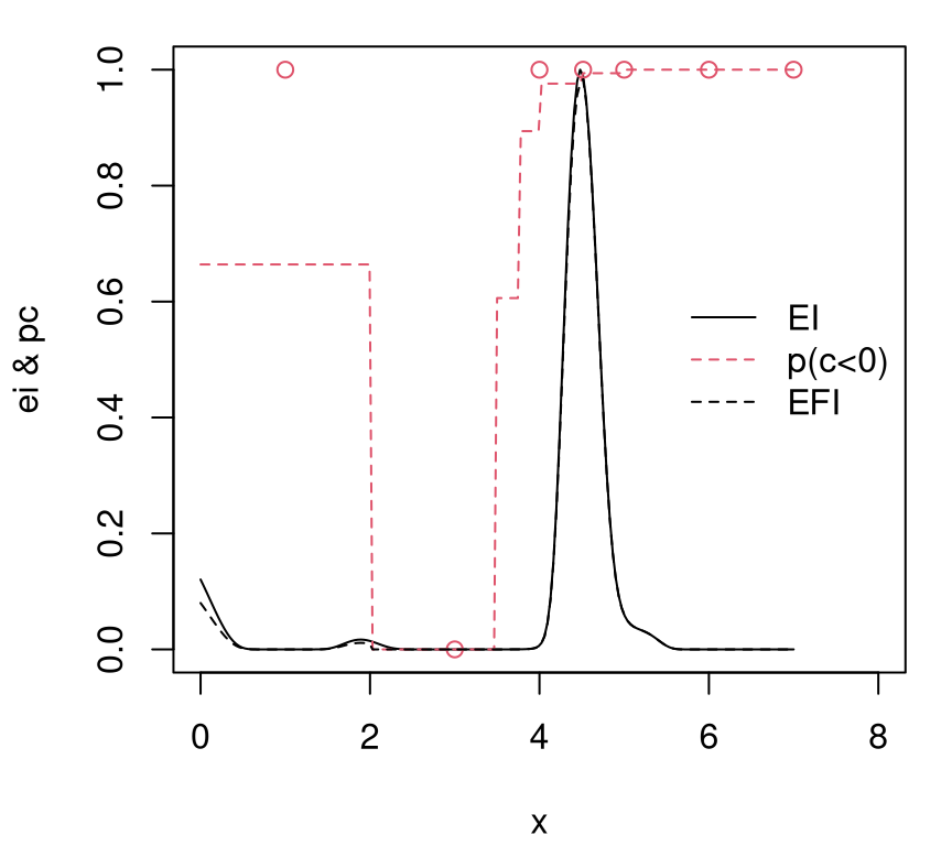
FIGURE 7.19: Second iteration of EFI following Figure 7.18.
In the version I’m viewing as I write this, updated surfaces strongly resemble those from the previous iteration (Figure 7.18) except perhaps with EI/EFI relatively higher on the valid side, i.e., that side not chosen for acquisition in the previous iteration. To fast-forward a little, R code below wraps our data augmenting, model updating and EFI-calculating from above into a for loop, selecting ten more evaluations in this fashion. Notice that jmleGP is used in this loop to tune lengthscales as well as nugget.
for(i in 1:10) {
m <- which.max(ei*pc)
X <- rbind(X, XX[m,])
y <- c(y, fsindn(XX[m,]) + rnorm(1, sd=0.15))
const <- c(const, as.numeric(XX[m,] > lc && XX[m,] < rc))
updateGP(gpi, X[nrow(X),,drop=FALSE], y[length(y)])
mle <- jmleGP(gpi, drange=c(eps, 2), grange=c(eps, var(y)), gab=ga$ab)
cfit <- randomForest(X, as.factor(const))
Xv <- X[const <= 0,,drop=FALSE]
fmin <- min(predGP(gpi, Xv, lite=TRUE)$mean)
pc <- predict(cfit, XX, type="prob")[,1]
ei <- EI(gpi, XX, fmin, pred=predGPnonug)
ei <- scale(ei, min(ei), max(ei) - min(ei))
}After choosing a total of twelve points beyond the seed space-filling design, Figure 7.20 shows the nature of \(p_n(x)\), EI and EFI from model fits based on a total of \(n = 17\) runs.
plot(XX, ei, type="l", xlim=c(0,8), ylim=c(0,1), xlab="x", ylab="ei & pc")
lines(XX, pc, col=2, lty=2)
points(X, 1 - const, col=2)
lines(XX, ei*pc, lty=2)
legend("right", c("EI", "p(c<0)", "EFI"), col=c(1,2,1),
  lty=c(1,2,2), bty="n")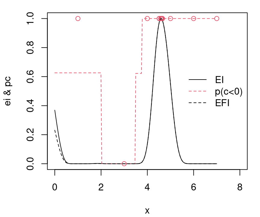
FIGURE 7.20: EFI view, ten more iterations after Figure 7.19.
That view reveals little to no exploration in the left half of the space, a behavior quite consistent across Rmarkdown builds. Although EI and EFI on the other side of the invalid region may increase in relative terms, it would take many right-side acquisitions before the criterion is maximized on the left. That’s a shame because, as Figure 7.21 reveals, the other side is definitely worth exploring.
p <- predGP(gpi, XX, lite=TRUE)
plot(XX, fsindn(XX), col="gray", type="l", lty=2)
points(X, y)
lines(XX, p$mean)
legend("top", c("truth", "mean"), col=c("gray", 1), lty=c(2,1), bty="n")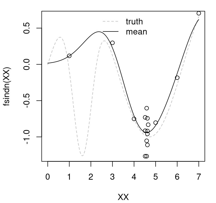
FIGURE 7.21: Final predictive mean (solid) fit to data (open circles), versus true surface (gray-dashed).
In the figure, black-open circles indicate sampled evaluations in the design, whereas the dashed-gray line is the truth. EFI’s exploration of the valid region was quite myopic in this instance.
Does IECI fare any better? Suppose we reinitialize the fit back at the same starting position (for a fair comparison) and go through the first couple of steps carefully with IECI, just as for EFI above. But first, don’t forget to free up the old GP fit.
deleteGP(gpi)
X <- X[1:ninit,,drop=FALSE]
y <- y[1:ninit]
const <- const[1:ninit]
gpi <- newGP(X, y, d=1, g=0.1*var(y), dK=TRUE)
mle <- mleGP(gpi, param="g", tmin=eps, tmax=var(y), ab=ga$ab)
cfit <- randomForest(X, as.factor(const))
pc <- predict(cfit, XX, type="prob")[,1]
Predictions from RF, obtained on the last line above, can be passed directly into ieciGP through its weight argument, w. The original IECI paper (Gramacy and Lee 2011) used a classification GP for \(p_n(x)\), coupled with an ordinary regression GP for IECI calculations in the plgp package. Sequential updating of both GPs is described in detail by Gramacy and Polson (2011). The ieciGP and ieciGPsep features in laGP are rather more generic, with a w argument allowing predicted probabilities to come from any classifier. Besides simplifying the narrative, we shall retain an RF classification surrogate here for a fairer benchmark against EFI. Readers curious about the original version are encouraged to inspect demos provided with plgp, in particular demo("plconstgp_1d_ieci").
Xv <- X[const <= 0,,drop=FALSE]
fmin <- min(predGP(gpi, Xv, lite=TRUE)$mean)
ieci <- ieciGP(gpi, XX, fmin, w=pc, nonug=TRUE)
ieci <- scale(ieci, min(ieci), max(ieci) - min(ieci))
Figure 7.22 shows the resulting surfaces. Since the seed design and responses are the same here as for EFI, the RF \(p_{n = 6}(x)\) surface is identical to Figure 7.18. For consistency with EI-based figures above, one minus IECI and \(c_i\) are shown.
plot(XX, 1 - ieci, type="l", xlim=c(0,8), ylim=c(0,1),
  xlab="x", ylab="ieci & pc")
lines(XX, pc, col=2, lty=2)
points(X, 1 - const, col=2)
legend("right", c("IECI", "p(c<0)"), col=c(1,2,2), lty=c(1,2,1), bty="n")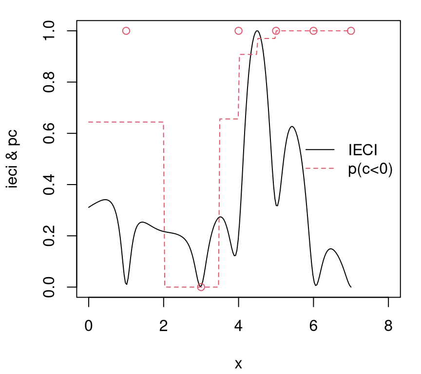
FIGURE 7.22: IECI analog of Figure 7.18.
By contrast with Figure 7.18, IECI is high on both sides of the invalid region. Moreover, IECI is smooth everywhere even though \(p_n(x)\) is piecewise constant. It’s never zero, although nearly so at the location of the solitary invalid input. IECI owes all three of those features, which are aesthetically more pleasing than the EFI analog, to its aggregate nature. A continuum of \(p_n(x)\)-values, as well as a continuum of conditional improvements, weigh in to determine which potential \(x_{n+1}\) offers the greatest promise for improvement in the valid region.
Code below selects the next point to minimize IECI, collects objective and constraint responses at that location, and augments the dataset.
m <- which.min(ieci)
X <- rbind(X, XX[m,])
y <- c(y, fsindn(XX[m,]) + rnorm(1, sd=0.15))
const <- c(const, as.numeric(XX[m,] > lc && XX[m,] < rc))
Next, the GP is updated and RF refit.
updateGP(gpi, X[ncol(X),,drop=FALSE], y[length(y)])
mle <- mleGP(gpi, param="g", tmin=eps, tmax=var(y), ab=ga$ab)
cfit <- randomForest(X, as.factor(const))
New IECI calculations are then derived from updated \(f_{\min}^n\) and \(p_n(x)\) evaluations.
Xv <- X[const <= 0,,drop=FALSE]
fmin <- min(predGP(gpi, Xv, lite=TRUE)$mean)
pc <- predict(cfit, XX, type="prob")[,1]
ieci <- ieciGP(gpi, XX, fmin, w=pc, nonug=TRUE)
ieci <- scale(ieci, min(ieci), max(ieci) - min(ieci))
Figure 7.23 shows the updated surfaces. Since both sides of the invalid region had high IECI in the previous iteration, it’s perhaps not surprising to see that IECI is now much higher on the side opposite to where the most recent acquisition was made.
plot(XX, 1 - ieci, type="l", xlim=c(0,8), ylim=c(0,1),
  xlab="x", ylab="ieci & pc")
lines(XX, pc, col=2, lty=2)
points(X, 1 - const, col=2)
legend("right", c("IECI", "p(c<0)"), col=c(1,2,2), lty=c(1,2,1), bty="n")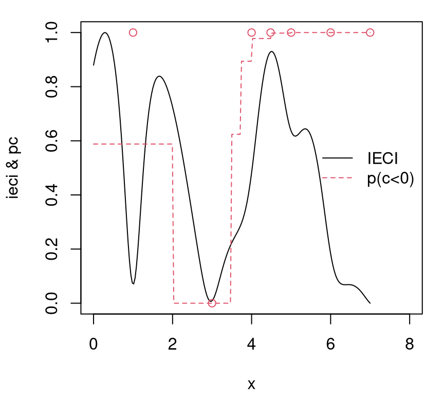
FIGURE 7.23: IECI updates after first IECI acquisition from Figure 7.22.
All right, lets see what happens when we do ten more steps like this, just as we did for EFI.
for(i in 1:10) {
  m <- which.min(ieci)
  X <- rbind(X, XX[m,])
  y <- c(y, fsindn(XX[m,]) + rnorm(1, sd=0.15))
  const <- c(const, as.numeric(XX[m,] > lc && XX[m,] < rc))
  updateGP(gpi, X[nrow(X),,drop=FALSE], y[length(y)])
  mle <- jmleGP(gpi, drange=c(eps, 2), grange=c(eps, var(y)), gab=ga$ab)
  cfit <- randomForest(X, as.factor(const))
  Xv <- X[const <= 0,,drop=FALSE]
  fmin <- min(predGP(gpi, Xv, lite=TRUE)$mean)
  pc <- predict(cfit, XX, type="prob")[,1]
  ieci <- ieciGP(gpi, XX, fmin, w=pc, nonug=TRUE)
  ieci <- scale(ieci, min(ieci), max(ieci) - min(ieci))
}
As shown in Figure 7.24, multiple evaluations have been taken on both sides of the invalid region. Sometimes, depending on the Rmarkdown build, runs are even taken within the invalid region. Compared to EFI, IECI has done a better job of exploring potential for improvement. Even after seventeen iterations, IECI is still high in appropriate places, on both sides of the invalid region. Surely it won’t be too many more iterations until the problem is nearly solved.
plot(XX, 1 - ieci, type="l", xlim=c(0,8), ylim=c(0,1),
  xlab="x", ylab="ieci & pc")
lines(XX, pc, col=2, lty=2)
points(X, 1 - const, col=2)
legend("right", c("IECI", "p(c<0)"), col=c(1,2,2), lty=c(1,2,1), bty="n")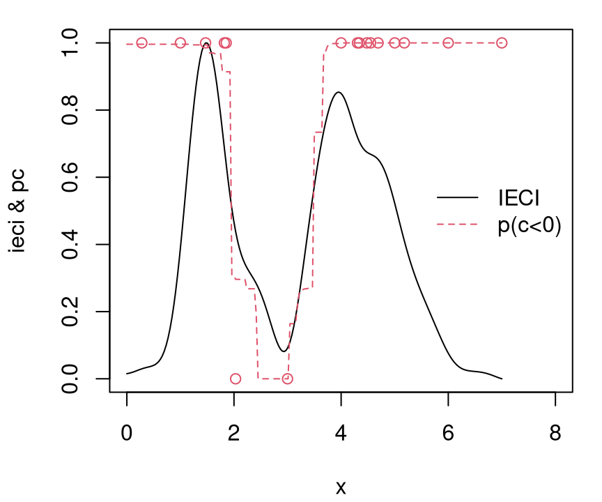
FIGURE 7.24: Acquisition surface after ten more IECI iterations; compare with Figure 7.20 for EFI.
The curious reader is encouraged to perform a few more iterations under both EFI and IECI acquisition functions. About 30 runs in total is sufficient for IECI to learn with confidence that the global (valid) minimum is on the left side of the input space. EFI takes rather more iterations, although differences between the two are by no means stark. Getting a good feel for how these two methods compare on this problem requires repeated experiments, in an MC fashion, to average over the random nature of the objective evaluations.
7.3.3 Real-valued constraints
Most often constraint functions are real-valued. Usually there are multiple such constraints. Paradoxically, this situation simplifies matters somewhat, because there are generally more modeling choices for real-valued simulations (e.g., GPs). Tractable nonlinear classifiers are somewhat harder to come by. Evaluations of \(c_n^{(j)}(x) \in \mathbb{R}\) provide extra information (compared to \(\{0,1\}\)), namely distance to feasibility. This can help accelerate convergence if used appropriately. But multiple constraints obviously make the overall problem more challenging: more things to model, making navigation toward valid optima a more complex enterprise.
EFI and IECI remain unchanged as general strategies as long as probability of constraint satisfaction \(p_n^{(j)}(x) = \mathbb{P}(c_n^{(j)}(x) \leq 0)\) can be backed out of fitted surfaces \(c_n^{(j)}(x)\) for each constraint \(j=1, \dots, m\).5 Under GPs, or any fitted response surface emitting Gaussian predictive equations, probabilities are readily available from the standard Gaussian CDF \(\Phi\), i.e., pnorm given \(\mu_n^{(j)}(x)\) and \(\sigma_n^{2(j)}(x)\)
\[ p_n^{(j)}(x) = \Phi\left(- \frac{\mu_n^{(j)}(x)}{\sigma_n^{(j)}(x)}\right). \]
Consequently EFI and IECI may utilize the magnitude of observed constraint values at best indirectly through \(\Phi\), and through the product \(\prod_{j=1}^m p_n^{(j)}(x)\) in the case of multiple constraints.
Sometimes constraints are where all the action is. So far in this chapter, focus has concentrated on the objective, with constraints being a nuisance. In many optimization problems constraints steal the show. Recall our motivating Lockwood groundwater remediation application from §2.4. The Lockwood objective is simple/known (e.g., linear), but simulation-based constraints require heavy computation, tracing out highly non-linear and non-convex valid regions. These create many deceptive local minima in the input domain. That can make for a hard search indeed.
Here’s a toy problem to fix ideas: a linear objective in two variables
\[\begin{equation} \min_{x} \left\{ x_1+x_2 : c_1(x) \leq 0, \, c_2(x) \leq 0, \, x\in [0,1]^2 \right\}, \tag{7.7} \end{equation}\]
where two non-linear constraints are given by
\[\begin{align} c_1(x) &= \frac{3}{2} - x_1 - 2x_2 - \frac{1}{2}\sin\left(2\pi(x_1^2-2x_2)\right) \tag{7.8} \\ \mbox{and} \quad c_2(x) &= x_1^2+x_2^2-\frac{3}{2}. \notag \end{align}\]
The function aimprob below, named for the American Institute of Mathematics (AIM) where it was cooked up (Gramacy et al. 2016), implements this toy problem as a blackbox. It was designed to synthesize many of the elements in play in problems such as Lockwood, yet in lower dimension and with a transparent and easy to evaluate form.
aimprob <- function(X, known.only=FALSE)
 {
  if(is.null(nrow(X))) X <- matrix(X, nrow=1)
  f <- rowSums(X)
  if(known.only) return(list(obj=f))
  c1 <- 1.5 - X[,1] - 2*X[,2] - 0.5*sin(2*pi*(X[,1]^2 - 2*X[,2]))
  c2 <- X[,1]^2 + X[,2]^2 - 1.5
  return(list(obj=f, c=drop(cbind(c1, c2))))
 }
A known.only argument allows “free” objective evaluations to be returned, if desired. This is required by one of our library implementations below. For now it may be ignored. While on the subject, however, even with known \(f(x) = x_1 + x_2\) this is a hard problem when \(c(x)\) is treated as an expensive blackbox. Figure 7.25 shows why. (The code chunk below first builds a plotting macro to quickly draw surfaces of this kind for use in later examples.) Colored contours show the objective. Being linear, the unconstrained global optimum is at the origin, however that location is deeply invalid. Red-dashed contours represent invalid regions; green-solid ones satisfy the constraint.
## establishing the macro
plotprob <- function(blackbox, nl=c(10,20), gn=200)
 {
  x <- seq(0,1, length=gn)
  X <- expand.grid(x, x)
  out <- blackbox(as.matrix(X))
  fv <- out$obj
  fv[out$c[,1] > 0 | out$c[,2] > 0] <- NA
  fi <- out$obj
  fi[!(out$c[,1] > 0 | out$c[,2] > 0)] <- NA
  plot(0, 0, type="n", xlim=c(0,1), ylim=c(0,1), xlab="x1", ylab="x2")
  C1 <- matrix(out$c[,1], ncol=gn)
  contour(x, x, C1, nlevels=1, levels=0, drawlabels=FALSE, add=TRUE, lwd=2)
  C2 <-  matrix(out$c[,2], ncol=gn)
  contour(x, x, C2, nlevels=1, levels=0, drawlabels=FALSE, add=TRUE, lwd=2)
  contour(x, x, matrix(fv, ncol=gn), nlevels=nl[1],
    add=TRUE, col="forestgreen")
  contour(x, x, matrix(fi, ncol=gn), nlevels=nl[2], add=TRUE, col=2, lty=2)
 }

## visualizing the aimprob surface(s)
plotprob(aimprob)
text(rbind(c(0.1954, 0.4044), c(0.7191, 0.1411), c(0, 0.75)),
  c("A", "B", "C"), pos=1)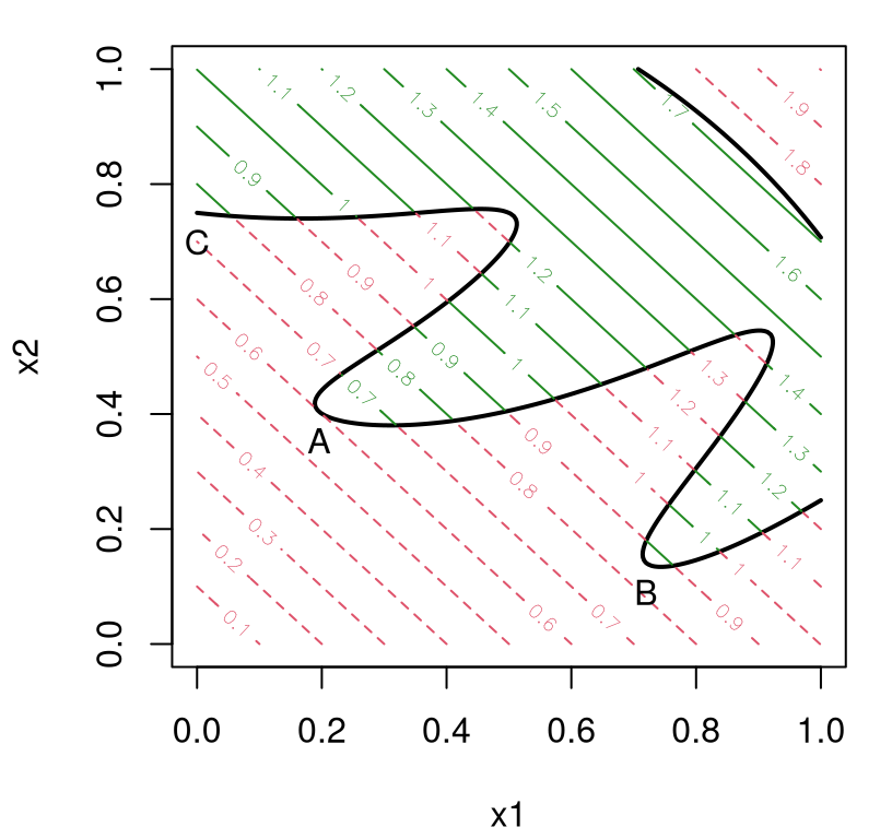
FIGURE 7.25: Linear objective (7.7) via contours colored by two nonlinear constraints (7.8). Locations of valid local minima are indicated by A, B and C.
Observe that there are three local minima, notated by points \(A\), \(B\), and \(C\), respectively. Coordinates of these locations are provided below.
\[ \begin{aligned} x^A &\approx [0.1954, 0.4044] & x^B &\approx [0.7191, 0.1411] & x^C &= [0, 0.75], \\ f(x^A) &\approx 0.5998 & f(x^B) &\approx 0.8609 & f(x^C) &= 0.75 \end{aligned} \]
Local optimum A is the global solution. A highly nonlinear \(c_1(x)\) makes for a challenging surface to optimize in search of minima. The second constraint, \(c_2(x)\) may seem uninteresting, but it reminds us that solutions may not exist on every boundary. In math programming jargon, \(c_2\) is a non-binding constraint. Search algorithms which place undue emphasis on boundary exploration could be fooled in the face of a plethora of non-binding constraints.
For problems like aimprob, techniques from the mathematical programming literature could prove quite valuable. Math programming has efficient algorithms for non-linear blackbox optimization under constraints with provable local convergence properties (see, e.g., Nocedal and Wright 2006), paired with lots of polished open source software. Whereas statistical approaches enjoy global convergence properties and excel when simulation is expensive, noisy, and non-convex, they offer limited support for constraints. Very few well-engineered libraries exist. There are almost none that handle blackbox constraints. Some kind of hybrid, leveraging math programming for constraints and statistical surrogates for global scope, could offer powerful synergy.
As somewhat of an aside, it’s perhaps telling of the current state of affairs in statistical (Bayesian) optimization that a special issue of the Journal of Statistical Software on Numerical Optimization in R: Beyond optim overlooks BO methods such as EI. Despite its many attractive properties, the word is not yet out in mainstream computational statistics circles. A partial explanation may be that statisticians can be cagey about releasing code, and implementation is essential to effective use of optimization methodology. Machine learners have released open Python libraries featuring EI with contributions from dozens of academic and industrial authors. For example, spearmint and MOE both offer limited support for constraints. A very nice exception in R is DiceOptim (Picheny, Ginsbourger, and Roustant 2016). Not coincidentally, DiceOptim implements some of the hybrids we’re about to discuss momentarily. As does laGP. Perhaps a JSS article featuring these packages is just around the corner.
7.3.4 Augmented Lagrangian
A framework ripe for hybridization with statistical surrogate-assisted optimization involves an apparatus called the augmented Lagrangian [AL; Bertsekas (2014)]. Also see Chapter 17 of Nocedal and Wright (2006). The AL is a composite of objective \(f(x)\) and vectorized constraint \(c(x)\):
\[\begin{equation} L_A(x;\lambda, \rho) = f(x) +\lambda^\top c(x) + \frac{1}{2\rho} \sum_{j=1}^m \max \left(0,c_j(x) \right)^2 \tag{7.9} \end{equation}\]
where \(\rho > 0\) is a penalty parameter, and \(\lambda \in \mathbb{R}_+^m\) serves as Lagrange multiplier. The formulation above is purely mathematical. Later when we introduce statistical surrogates we’ll bring back \(n\) subscripts, etc.
An AL optimization utilizes the AL composite (7.9) to transform a constrained optimization problem into a sequence of simply constrained ones. Solutions \(x^\star = \mathrm{argmin}_x L_A(x; \lambda, \rho)\) to the so-called “AL subproblem”, can guide an optimizer toward solutions to the original problem (7.6) through a dynamically determined sequence of \(\lambda\) and \(\rho\)-values. Basically, a schedule of delicate increases to \(\lambda\) and \(\rho\) when \(x^\star\) is invalid, as detailed in Algorithm 7.1, coaxes subproblems toward valid optima. Omitting the Lagrange multiplier term \(\lambda^\top c(x)\) leads to (an example of) a so-called additive penalty method (APM) composite.
\[ \mathrm{APM}(x;\rho) = f(x) + \frac{1}{2\rho} \sum_{j=1}^m \max \left(0,c_j(x) \right)^2 \]
Without considerable care in choosing the form and scale of penalization \((\rho)\), APMs can introduce ill-conditioning in the resulting subproblems. By introducing Lagrange multiplier \(\lambda\), working together with penalty \(\rho\) to define the subproblem, with automatic updates as the method iterates, local convergence can be guaranteed under relatively mild conditions.
Many of the details are provided by Algorithm 7.1. There are basically two steps: 1) optimize the subproblem; and 2) update parameters \((\lambda, \rho)\).
Algorithm 7.1: Augmented Lagrangian Constrained Optimization
Assume the search region is \(\mathcal{X}\), perhaps a unit hypercube.
Require a blackbox evaluating \(f(x)\) and vectorized \(c(x)\) jointly; initial values \(x^0\), \(\lambda^0\) and \(\rho^0\), and maximum number of “outer loop” iterations \(k_{\max}\).
For \(k=1,\dots,k_{\mathrm{max}}\) comprising the “outer loop”:
- “Inner loop”: approximately solve the subproblem:
\[ x^k = \mbox{arg}\min_{x\in\mathcal{X}} \left\{ L_A(x;\lambda^{k-1},\rho^{k-1}) : x\in \mathcal{X}\right\}. \]
- Update:
- \(\lambda_j^k = \max\left(0,\lambda_j^{k-1}+\frac{1}{\rho^{k-1}} c_j(x^k) \right)\), for \(j=1, \ldots, m\);
- if \(c(x^k)\leq 0\), set \(\rho^k=\rho^{k-1}\); otherwise, set \(\rho^k=\frac{1}{2}\rho^{k-1}\).
End For
Return \(x^{k_{\mathrm{max}}}\), the solution to the most recently solved subproblem.
While most of the work is in Step 1, off-loading the subproblem to an ordinary optimizer ("L-BFGS-B"), the action is all in Step 2. Updates of \(\lambda\) and \(\rho\) serve to nudge subproblems toward good and valid local evaluations of the objective function. When \(x^k\) satisfies all constraints, i.e., \(c(x^k) \leq 0\) meaning that all components of that vectorized logical statement are true, the penalty parameter \(\rho\) is unchanged and \(\lambda\) moves closer to zero, if not identically so. This situation is akin to the overall scheme being “on the right track”. On the other hand, if any of the constraints are not satisfied, i.e., some \(c_j(x^k) > 0\), then the corresponding components of the Lagrange multiplier \(\lambda_j\) are increased, and the penalty \(1/\rho\) doubles. This is like a course correction from Chapter 3.
Although updates of \((\lambda, \rho)\) from one iteration to the next are key, the range specified for the “outer (for) loop” in the algorithm isn’t much more than window dressing. A presumption that there’s a budget \(k_{\max}\) is somewhat unrealistic, as the real expense lies in the evaluations which happen in the “inner loop” of Step 1, solving the subproblem. Determining convergence within the inner loop [Step 2], is highly dependent on the choice of inner loop solver. Thankfully, theory for global convergence of the overall AL scheme is forgiving about criteria used to end each inner loop search. As long as some progress is made on the subproblem, perhaps to economize on the number of blackbox evaluations, convergence is eventually guaranteed – although not necessarily before exhausting a run budget. The AL framework for constrained optimization is robust to inner loop dynamics in this sense.
That state of affairs is rather akin to expectation maximization (EM), to choose an example more familiar to a statistical audience. EM will converge even if the M-step is inefficient. As long as progress can be made, increasing the (E)xpected log likelihood rather than fully (M)aximizing it, outer iterations between E- and M-steps will converge to a local optima of the observed data log likelihood.
When reducing evaluations of expensive blackbox functions is less of a concern, outer loop convergence may be called when all constraints are satisfied and the (approximated) gradient of the Lagrangian is sufficiently small; for example, given thresholds \(\eta_1,\eta_2\geq 0\), one could stop when
\[ \left \|\max\left\{c(x^k),0\right\}\right\| \leq \eta_1 \qquad \mbox{and} \qquad \left\|\nabla f(x^k)+\sum_{j=1}^m \lambda_i^k \nabla c_j(x^k)\right\|\leq \eta_2. \]
Presuming that blackbox run budgets preclude iterating exhaustively until convergence, a more pragmatic return value (compared to what’s prescribed in Algorithm 7.1) may be warranted. The final subproblem solution, \(x^{k_{\mathrm{max}}}\), could well be invalid if a budget short-circuits search. Instead it’s safer to report \(x^\star\) yielding the BVV \(y^\star = f(x^\star)\) of the objective recorded so far. Within the inner loop, where blackbox evaluations of \(f\) and \(c\) are made in pursuit of a subproblem solution, simply update \((x^\star, y^\star) \leftarrow (x, y)\) whenever \(y = f(x) \leq y^\star\) and \(c(x) \leq 0\) are encountered.
To illustrate, consider the following application on our toy aimprob (7.7)–(7.8). Setting up the subproblem solved in Step 2 of Algorithm 7.1, the code below wraps an arbitrary blackbox (e.g., aimprob) in AL clothes. A variable in the global environment, evals, is updated to keep track of the number of blackbox evaluations within the inner loop.
ALwrap <- function(x, blackbox, B, lambda, rho)
 {
  if(any(x < B[,1]) | any(x > B[,2])) return(Inf)
  fc <- blackbox(x)
  al <- fc$obj + lambda %*% fc$c +
    rep(1/(2*rho), length(fc$c)) %*% pmax(0, fc$c)^2
  evals <<- evals + 1
  return(al)
 }
The beauty of constrained optimization by AL is how easy it is to code the outer loop, as long as that a good unconstrained optimization library is on hand to handle the inner loop. For our illustration, we’ll keep it simple and use the default method="Nelder-Mead" from optim, acting directly on blackbox (i.e., aimprob) through ALwrap. Since that method doesn’t support bound constraints, bounding box checking against argument B (the analog of our search region/input domain \(\mathcal{X}\) from earlier in the chapter) is essential as a first step in the wrapper above. Combining those elements and the updates to \((\lambda, \rho)\), the function below implements the entirety of Algorithm 7.1.
ALoptim <- function(blackbox, B, start=runif(ncol(B)),
  lambda=rep(0, ncol(B)), rho=1/2, kmax=10, maxit=15)
 {
  ## initialize AL wrapper
  evals <- 0
  formals(ALwrap)$blackbox <- blackbox

  ## initialize outer loop progress
  prog <- matrix(NA, nrow=kmax + 1, ncol=nrow(B) + 1)
  prog[1,] <- c(start, NA)

  ## "outer loop" iterations
  for(k in 1:kmax) {

    ## solve subproblem ("inner loop")
    out <- optim(start, ALwrap, control=list(maxit=maxit),
      B=B, lambda=lambda, rho=rho)

    ## extract the x^* that was found, and keep track of progress
    start <- out$par
    fc <- blackbox(start)
    prog[k+1,1:ncol(B)] <- start
    if(all(fc$c <= 0)) prog[k+1,ncol(B)+1] <- fc$obj

    ## update augmented Lagrangian parameters
    lambda <- pmax(0, lambda + (1/rho)*fc$c)
    if(any(fc$c > 0)) rho = rho/2
  }

  ## collect for returning
  colnames(prog) <- c(paste0("x", 1:ncol(B)), "obj")
  return(prog)
}
The only required arguments are blackbox, written in a form amenable to wrapping in ALwrap as exemplified by aimprob, and study region \(\mathcal{X} \equiv\) B. Sensible defaults are provided for the other tunable parameters, at least as a jumping-off point. Notice that maxit=15 limits the inner loop to fifteen iterations, however the number of blackbox evaluations may be much greater than that depending on how the inner loop attacks the subproblem. Also notice that an extra blackbox call is made outside of optim to extract the constraint evaluation at the solution to the subproblem. A more clever implementation, working with a custom inner loop optimizer that saves function evaluations, might be able to avoid this redundant, potentially expensive, evaluation. Likewise, the implementation tracks the best valid subproblem solution, rather than the best of all valid evaluations (BVV).
Let’s see how ALoptim works on aimprob with a somewhat pathological initialization: about as far as you can get from any of the valid local minima.
evals <- 0
B <- matrix(c(rep(0,2), rep(1,2)), ncol=2)
prog <- ALoptim(aimprob, B, start=c(0.9, 0.9))
Figure 7.26 illustrates progress by plotting outer loop iteration number (plus one for the starting location), with “cross-hairs” at the final value to ease visualization.
plotprob(aimprob)
text(prog[,1], prog[,2], 1:nrow(prog))
m <- which.min(prog[,3])
abline(v=prog[m,1], lty=3, col="gray")
abline(h=prog[m,2], lty=3, col="gray")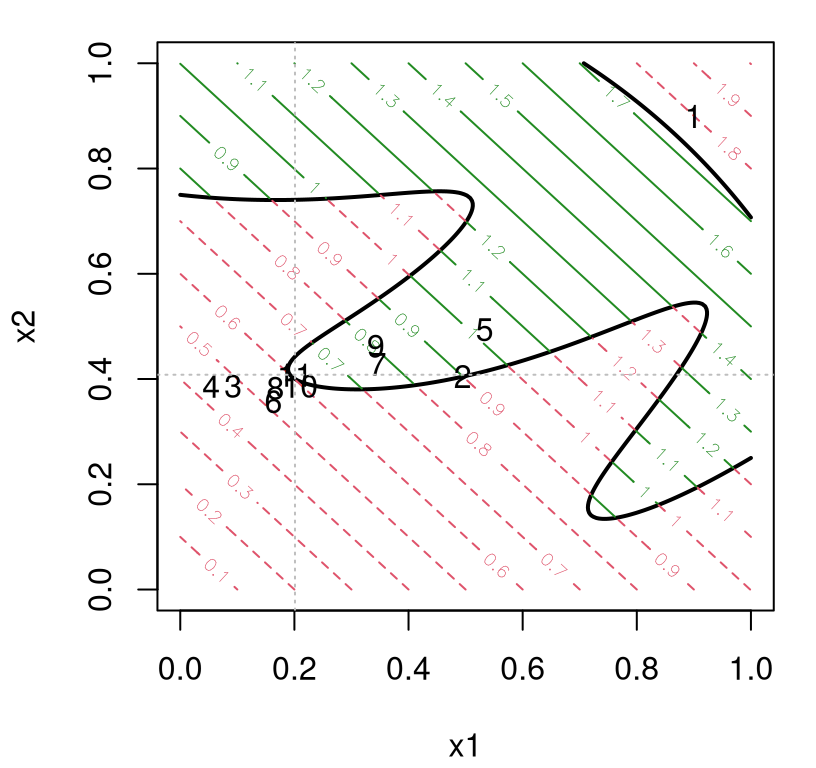
FIGURE 7.26: One application of optimization by augmented Lagrangian. The numbers indicate \(k\) at location \(x^k\) solving the AL subproblem. Cross-hairs highlight the final solution.
It would appear that after just ten outer loop iterations the global solution has been found, at least to within a decent tolerance. However, this summary hides a huge computational expense in terms of the number of blackbox evaluations.
## [1] 168This situation could potentially have been much worse with a higher value of maxit. To what extent might one improve upon this state of affairs? Before heading down that road, consider first what happens when we randomly reinitialize at a few more places.
reps <- 30
all.evals <- rep(NA, reps)
start <- end <- matrix(NA, nrow=reps, ncol=2)
for(i in 1:reps) {
  evals <- 0
  prog <- ALoptim(aimprob, B, kmax=20)
  start[i,] <- prog[1,-3]
  m <- which.min(prog[,3])
  end[i,] <- prog[m,-3]
  all.evals[i] <- evals
}
To ensure that a good answer is obtained in each repetition, a higher number of outer loop iterations, kmax=20, is used. Figure 7.27 shows the (random) starting and best valid ending value of the objective from each repetition as arrows.
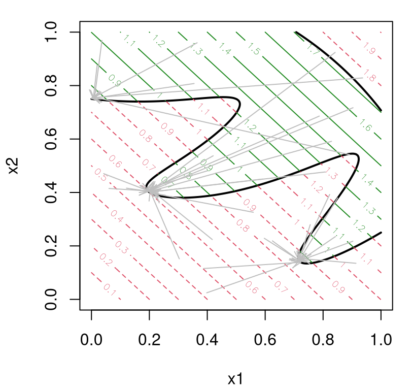
FIGURE 7.27: Outcome of repeated applications of AL-optimization. The origin of each arrow indicates a randomly chosen initialization; terminus indicates the outcome of search.
It’s quite clear from this view that the AL is adequately finding local solutions, but sometimes it’s surprising what local solution it finds. In at least one occasion out of thirty, the ending value lands in a trough that’s both farther away from its starting location and traverses shallower gradients in order to do so. So while local AL convergence is fairly robust to subproblem progress in inner loop iterations, it can be hard to predict which of several local (valid) optima it’ll converge to. And all that while spending frivolously on blackbox evaluations, at least compared to what I’m about to propose momentarily.
##    Min. 1st Qu.  Median    Mean 3rd Qu.    Max.
##     244     332     337     322     339     340
For a more interactive variation on the above illustration, see aimprob.R. This demo allows the user to step through outer loop iterations, under random initialization, to get a better feel for how an AL guides search. An attentive reader will notice from the demo that the AL method often approaches valid solutions from the invalid side of constraint boundaries, with at least as many evaluations in invalid as valid regions – a behavior well-studied in the literature. As a result, many software libraries implementing AL composites (7.9) consider as solutions \(x^\star\) those inputs corresponding to the BOV whose constraints are within an \(\epsilon\) tolerance of valid (e.g., \(c(x^\star) \leq 1e^{-4}\)). Others feel that it’s safer to simply report the BVV of the objective.
The calculation below shows that solutions to the subproblem, the \(x^k\)s, are about equally likely to be valid as invalid on this problem, which can be interpreted as a symptom of that behavior.
## [1] 0.4286Without a cache of the entirety of blackbox evaluations, and without a much larger maxit and kmax, it’s difficult to illustrate this phenomenon in greater detail. Of course, we don’t want to dwell too much here on review of math programming methods. The takeaway message is that the AL method is a potentially expensive, local affair, that otherwise has many nice empirical and theoretical properties. And it’s quite easy to implement.
7.3.5 Augmented Lagrangian Bayesian optimization (ALBO)
Since the inner loop solver can be anything, as long as it makes progress on the subproblem, why not try a surrogate-assisted/BO solver? That might be the best of both worlds. Surrogate methods enjoy global scope, heuristics like EI are good at navigating exploration–exploitation trade-offs, and setups adapted to the constrained setting are few. AL methods converge to valid solutions, but are profligate with blackbox evaluations despite their distinctly local scope. This idea, of combining the AL with Bayesian optimization (BO) was originally proposed by Gramacy et al. (2016), and later dubbed ALBO by Picheny et al. (2016) who extended the methodology to equality and mixed (inequality and equality) constraints.
The crux of the approach involves training a surrogate, which will ultimately guide the inner loop, on the entire corpus of blackbox evaluations obtained so far, i.e., over all inner and outer iterations of the loops in Algorithm 7.1. Whereas in a more conventional AL approach, each subproblem would be solved without any memory of solvers run in earlier outer loop iterations. Not only that, but typically inner loop optimizers (like those from optim) are themselves also memoryless, or at best have limited memory like "L-BFGS-B". Therefore the proposed application of surrogates here represents a regime shift in the modus operandi compared to canonical AL methodology. Surrogate-based inner loops will have not only global scope on the specific subproblems they’re solving, but also knowledge of the surface(s) gathered from previous subproblems.
Suppose that \(n\) such evaluations of the blackbox have been made so far, across all inner and outer loops of Algorithm 7.1. Denote by
\[ D_n = (x_1, f(x_1), c(x_1)), \dots, (x_n, f(x_n), c(x_n)) \]
the data available for training surrogates. We’ve been largely able to avoid double-indexing so far in this chapter, over constraint coordinates \(j=1,\dots,m\) and observation indices \(i=1,\dots,n\). (In some places I was downright sloppy, but context – usually a 1d constraint – helped.) Going forward, I shall invest in more precise notation. Let \(c_j^{(i)}\) be the \(j^{\mathrm{th}}\) coordinate of \(c(x_i)\), the vector of constraint evaluations from the \(i^{\mathrm{th}}\) run of the blackbox. To have notation match for objective evaluations, even though they’re not vectorized, I shall write \(f^{(i)}\) as a shorthand for \(f(x_i)\). So our training data can now be more compactly notated as \(D_n = \{(f^{(i)}, c^{(i)}\}_{i=1}^n\) for \(m\)-vectors \(c^{(i)}\). As usual, focus is on GP surrogates for \(D_n\), although much of the discussion is agnostic about that choice with the caveat that a few of the closed-form results leverage Gaussian predictive equations.
There are several options for how exactly to proceed, as regards modeling data \(D_n\) in a means effective for solving subproblems in Step 1 at each iteration \(k\). One is easy to rule out. Perhaps it’s strange to begin by focusing attention on a flawed notion. But there’s good reason for doing so. It represents a rather straightforward approach; the first thing one might think to try. Ultimately it serves to illustrate pitfalls in use of GP surrogates in practice, whether for optimization or otherwise. You might call it the gestalt approach: model the whole rather than the sum of its parts. Let \(y_i = L_A(x_i; \lambda^{k-1}, \rho^{k-1})\) via \(f^{(i)}\) and \(c^{(i)}\). That is,
\[ y_i = f^{(i)} +(\lambda^{k-1})^\top c^{(i)} + \frac{1}{2\rho^{k-1}} \sum_{j=1}^m \max \left(0,c_j^{(i)} \right)^2. \]
Then fit a surrogate to \((x_1, y_1), \dots, (x_n, y_n)\) in the usual way, and guide the inner loop search using your preferred acquisition function: predictive mean (EY), EI, IECI, etc.
Benefits to this scheme are immediately self-evident. Foremost, it’s highly modular. Plug in any (objective-only) surrogate-assisted optimizer trained on \(y_i\)’s, whether of your own design, borrowing one of the functions provided earlier, or from an existing library. Such a scheme ought to have many desirable features. It’ll enjoy global scope, being trained on all data encountered so far. Yet it’ll also act locally: the AL method focuses search on promising parts of the input space from the perspective of satisfying constraints. This hybrid scheme would seem to embody an attractive means of balancing exploration, exploitation, constraint satisfaction, and (perhaps above all) simple implementation.
So what’s the problem? The biggest issue is that the response surface created by mapping \(D_n \rightarrow \{(x_i, y_i)\}_{i=1}^n\) possesses two pathologies known to thwart effective spatial modeling, all wrapped into a tidy package. The squared term creates inherent nonstationarity by amplifying dynamics away from valid regions. The \(\max\) creates kinks in the surface, breaking smoothness. Although it’s definitely possible to engineer a covariance kernel, for GP modeling say, that anticipates response surface features such as these, I know of none readily available for such purposes.
A somewhat smaller issue is one of efficiency. The AL composite (7.9) takes on a quadratic form of sorts, yet that information isn’t leveraged in the surrogate model specification. Again, at least not if a canonical, library-based GP modeling is deployed. In situations where \(f\) is known, for example linear in our toy aimprob and Lockwood problems, the apparatus would needlessly model a known quantity. Many challenging problems have known objectives, so that special case ought to be explicitly acknowledged by the methodological development. In fairness, classical AL doesn’t leverage a known quadratic form or a potentially known objective either. Yet more specialized setups have been proposed in the literature, paying dividends in practice (Kannan and Wild 2012). Since we’re drawing up schematics for something new, why not lay out the full wish-list at the very start?
All of these shortcomings are addressed simultaneously by separately/independently surrogate modeling each component of the AL. That is, fit a surrogate to the objective data \(\{(x_i, f^{(i)})\}_{i=1}^n\), if needed, and fit \(m\) separate surrogates to \(\{x_i, c_j^{(i)}\}_{i=1}^n\) for each of \(m\) constraints. As shorthand, write \(f^n\) for fitted objective surrogate, and \(c^n= (c_1^n, \dots, c_m^n)\) for mutually independent fitted constraint surrogates. Let \(Y_f(x) \equiv Y_{f^n}(x) \sim f^n\) denote a random variable characterizing predictive uncertainty at novel input \(x\) under the objective surrogate, which may simply be \(y_f(x) = f(x)\) if the objective is treated as known. Similarly, let \(c^n = (c_1^n, \dots, c_m^n)\) emit predictive random variables \(Y_c(x) \equiv Y_c^n(x) = (Y_{c_1}^n(x), \dots, Y_{c_m}^n(x))\) following the distribution of novel predictions under the \(m\) constraint surrogates. Then, the distribution of the composite random variable
\[\begin{equation} Y(x) = Y_f(x) + \lambda^\top Y_c(x) + \frac{1}{2\rho} \sum_{j=1}^m \max(0, Y_{c_j}(x))^2 \tag{7.10} \end{equation}\]
can serve as a surrogate for \(L_A(x; \lambda, \rho)\).
What can you do with this composite random variable? If surrogate predictive equations are Gaussian, as they are from fitted GPs, then the AL composite posterior mean (EY) is available in closed form.
\[ \mathbb{E} \{ Y(x)\} = \mu_f^n(x) + \lambda^\top \mu_c^n(x) + \frac{1}{2\rho} \sum_{j=1}^m \mathbb{E}\{ \max(0, Y_{c_j}(x))^2\} \]
A result from generalized EI (Schonlau, Welch, and Jones 1998) furnishes a closed form for the expectation inside that sum above. Specifically, an expression for \(\mathbb{E}\{ \max(0, Y_{c_j}(x))^2\}\) follows by recognizing its argument as a powered improvement for \(-Y_{c_j}(x)\) over zero, that is, \(I^{(0)}_{-Y_{c_j}}(x) = \max\{0, 0 + Y_{c_j}(x)\}\). Since the power is 2, an expectation-variance relationship can be exploited to obtain
\[ \begin{aligned} & \mathbb{E} \{ \max(0, Y_{c_j}(x))^2\} = \mathbb{E}\{I_{-Y_{c_j}}^{(0)}(x)\}^2 + \mathbb{V}\mathrm{ar}[I_{-Y_{c_j}}^{(0)}(x)] \\ &= \sigma^{2n}_{c_j}(x)\left[\left( 1+ \left(\frac{\mu^n_{c_j}(x)}{\sigma_{c_j}^n(x)}\right)^{2}\right) \Phi\left(\frac{\mu^n_{c_j}(x)}{\sigma_{c_j}^n(x)} \right) +\frac{\mu^n_{c_j}(x)}{\sigma_{c_j}^n(x)} \phi\left(\frac{\mu^n_{c_j}(x)}{\sigma_{c_j}^n(x)} \right) \right]. \end{aligned} \]
It’s hard to imagine many other quantities relevant for optimization taking on analytic closed forms. The \(\max\) in the AL composite random variable (7.10) is hard to work around. We got lucky with the mean above. Variances may similarly be available, enabling LCB-based acquisition (7.1), however theoretical guidance for choosing appropriate weights \(\beta_n\) in this AL context isn’t readily available. The simplest way to evaluate EI under the composite AL is through MC. Sample \(T\) deviates \(y_f^{(t)}(x)\) and \(y_c^{(t)}(x)\), form \(y^{(t)}(x)\) through Eq. (7.9), and average:
\[\begin{equation} \mathrm{EI}(x) \approx \frac{1}{T} \sum_{t=1}^{T} \max\{0, y_{\mathrm{min}}^n - y^{(t)}(x)\}. \tag{7.11} \end{equation}\]
Surprisingly, this works quite well in practice and even applies when surrogates emit non-Gaussian predictors. \(T\) as small as 100 is often sufficient to achieve stable relative EI comparisons in \(\mathcal{X}\)-space. Such crude numerical approximation can actually be better, in terms of cost-benefit trade-off, than other fancier alternatives. This is borne out in our empirical work. But hold that thought for a moment.
A big downside to MC-based acquisition is lack of determinism. Stochastic optimization dulls the deliberate weighing of trade-offs that an expensive blackbox deserves. Perhaps more practically, an MC EI is hard to meta-optimize, say through an optim subsubroutine. After all, optim-like inability to cope with noisy evaluations was one of the big motivators for BO alternatives.
What alternatives? Well if the story ended there, this whole ALBO thing would be somewhat underwhelming. Although the \(\max\) thwarts analytics, there’s a well-known technique from math programming for softening such hard thresholds. One can equivalently reformulate AL subproblems without the \(\max\) by introducing so-called slack variables. The setup is as follows. Introduce \(s_j\), for \(j=1,\dots,m\), i.e., one for each \(c_j(x)\); convert inequality into equality constraints: \(c_j(x) - s_j = 0\); and augment the program with additional bound constraints \(s_j \geq 0\), for \(j=1,\dots, m\). In practice these latter, simply defined constraints are subsumed into the box \(\mathcal{B} = \mathcal{X} \times \mathcal{S}\) where \(\mathcal{S} = [0,\infty]^m\). In this way, the problem is mapped from \(p\)-dimensional \(\mathcal{X}\) space to \((p + m)\)-dimensional \(\mathcal{X} \times \mathcal{S}\) space. Although our focus here is on inequality constrained problems, it’s worth commenting that equality (and thus mixed constraints) are implemented by fixing \(s_j = 0\) for relevant coordinates, \(j\), of the constraint vector.
Slack-equality-based AL is sometimes presented as the canonical form in textbooks (Nocedal and Wright 2006, chap. 17) because that framework can accommodate both equality and inequality constraints, even simultaneously. Introducing slacks into ALBO, as described above, facilitates the only known EI-based method for handling mixed (equality and inequality) constraints (Picheny et al. 2016) in surrogate-assisted/BO literatures. But I’ll try not to unduly complicate the narrative here by over-emphasizing the mixed constraints setting. Instead, let’s focus on using slacks to reformulate the ALBO composite random variable (7.10), with an eye toward a more analytical EI calculation.
Picheny et al. (2016) showed that, for the slack-inequality constrained problem, the AL composite becomes
\[\begin{align} L_A(x, s; \lambda, \rho) &= f(x) + \lambda^\top (c(x) + s) + \frac{1}{2\rho} \sum_{j=1}^m (c_j(x) + s_j)^2, \quad \mbox{ so that} \notag \\ Y(x,s) &= Y_f(x) + \sum_{j=1}^m \lambda_j s_j + \frac{1}{2\rho} \sum_{j=1}^m s_j^2 + \frac{1}{2\rho} \sum_{j=1}^m \left[\left( \alpha_j + Y_{c_j}(x) \right)^2 - \alpha_j^2 \right], \tag{7.12} \end{align}\]
where \(\alpha_j= \lambda_j\rho + s_j\). Observe that if \(s_j = 0\), encoding an equality constraint, the quadratic penalty eventually forces \(c_j(x) = 0\) with small enough \(\rho\).
It’s helpful to re-arrange the expression for \(Y(x,s)\) in Eq. (7.12) in order to focus on interplay between slacks \(s\) and ordinary inputs \(x\). Let \(g(s) = \sum_{j=1}^m \lambda_j s_j + \frac{1}{2\rho} \sum_{j=1}^m s_j^2 - \alpha_j^2\) capture the part of \(Y(x,s)\) which is a function of slacks \(s\) only, and let \(W(x,s) = \sum_{j=1}^m [( \alpha_j + Y_{c_j}(x))^2]\) capture that which depends on both types of inputs. With those definitions, we may more compactly write
\[ Y(x, s) = Y_f(x) + g(s) + \frac{1}{2\rho} W(x, s). \]
Using \(Y_{c_j} \sim \mathcal{N} \left(\mu_{c_j}(x), \sigma_{c_j}^2(x) \right)\), \(W\) can be written as
\[ \begin{aligned} W(x, s) &= \sum_{j=1}^m Z_j^2, && \mbox{with } & Z_j &\sim \mathcal{N}\left(\mu_{c_j}(x) + \alpha_j, \sigma^2_{c_j}(x) \right)\\ &= \sum_{j=1}^m \sigma^2_{c_j}(x) \bar{Z}_j^2, && \mbox{with } & \bar{Z}_j &\sim \mathcal{N}\left(\frac{\mu_{c_j}(x) + \alpha_j}{\sigma_{c_j}(x)}, 1 \right)\\ &= \sum_{j=1}^m \sigma^2_{c_j}(x) X_j, && \mbox{with } & X_j &\sim \chi^2_{\nu=1} \left( \left( \frac{\mu_{c_j}(x) + \alpha_j}{\sigma_{c_j}(x)}\right)^2 \right), \end{aligned} \]
where that final random variable is a weighted sum of non-central chi-square (WSNC) variates (Duchesne and Micheaux 2010). WSNC density, distribution and quantile functions are provided by R packages CompQuadForm (de Micheaux 2017) and sadists (Pav 2017).
Those library functions – for CDF evaluation in particular – enable EI approximation to a high degree of accuracy with straightforward numerics. Under the AL-composite, that involves working with \(\mathrm{EI}(x, s) = \mathbb{E} \left[\left( y_{\min}^n - Y(x, s) \right) \mathbb{I}_{\{Y(x, s) \leq y_{\min}^n\}} \right]\), given the current minimum \(y^n_{\min}\) of the AL over all \(n\) runs. Consider the somewhat simpler case where \(f(x)\) is treated as known. Let \(w^n_{\min} = 2\rho \left(y^n_{\min} - f(x) - g(s)\right)\), and \(D_W\) denote the WSNC (cumulative) distribution of \(W(x,s)\). It can be shown that
\[ \begin{aligned} \mathrm{EI}(x, s) &= \frac{1}{2\rho} \mathbb{E} \left[ \left( w^n_{\min} - W(x,s) \right) \mathbb{I}_{W(x,s) \leq w^n_{\min}} \right] \\ &= \frac{1}{2\rho} \int_{-\infty}^{w^n_{\min}} D_W(t) \; dt = \frac{1}{2\rho} \int_{0}^{w^n_{\min}} D_W(t) \; dt. \end{aligned} \]
In other words, EI calculation involves a one-dimensional definite integral whose integrand may be evaluated with a library subroutine. For example, if wts is a vector holding the \(m\) components of \(\sigma_{c_j}^2(x)\), and ncp holds arguments of \(\chi_{\nu=1}^2(\cdot)\) above, i.e.,
\[ \mathrm{ncp}_j = \left(\frac{\mu_{c_j}(x) + \alpha_j}{\sigma_{c_j}(x)}\right)^2, \]
then the following commands yield EI under the AL composite.
R ex> library(sadists)
R ex> obj.EI <- function(t)
+       psumchisqpow(q=t, wts, rep(1, m), ncp, rep(1, m))
R ex> EI <- integrate(obj.EI, 0, wmin)$value / (2*rho)
Note these lines are just an example; that R code is not included in the Rmarkdown build in order to produce any output shown here or below. For more details, see Appendix C of the arXiv version of Picheny et al. (2016), which illustrates both sadists and CompQuadForm application. A worked example involving those calculations under the hood will be provided momentarily. Adjustments are trivial when \(f\) is treated as unknown; see
Picheny et al. (2016) for details. An example for that case is coming soon too. It’s worth acknowledging that the scheme outlined above is still numeric. However, unlike the MC version (7.11), which collected random deviates in \(m+1\) dimensions, the numerics here are in 1d. Simple quadrature suffices, like that implemented by integrate in base R, which provides approximations to tolerances low enough to meta-optimize, with optim say.
7.3.6 ALBO implementation details
Before jumping headlong into illustrations, several details are worthy of lip service. The attentive reader may have noticed some logical gaps in the passages above, and may have justifiably been worried they were being swept under a rug. Two are engineering details: a choice of initializing \((\lambda^0, \rho^0)\); and how to determine inner loop convergence of the surrogate-assisted sub-solver. I shall summarize default solutions to these which work well, but could potentially be sub-optimal in particular settings. Two others involve the slack re-formulation and are more technical, in the sense that there’s a right way from a certain point of view. The first involves re-describing Algorithm 7.1 for slacks. Changes here are largely semantic, however the crucial step of updating \((\lambda^k, \rho^k)\) requires explicit adjustment. Finally, although slack variables expand the search space by up to \(m\) dimensions, one additional per constraint beyond the dimension of \(x\), an optimal setting of \(s_j^k\) can be expressed as a function of \(x\), mapping the search space back down again to the dimension of \(x\) only.
A sensible initialization strategy for \((\lambda^0, \rho^0)\) balances the scales of objective and constraint in the AL on the basis of outputs obtained from a seed space-filling design of size \(n_0\). The description here, and in the following passages, favors generality with respect to a mixed (inequality and equality) constraint setting. Let \(v(x)\) be a logical vector of length \(m=m_{\leq}+m_{=}\) recording the validity of \(x\) in a zero-slack setting. Let \(v_j(x) = 1\) if the \(j^{\mathrm{th}}\) inequality constraint is satisfied, \(c_j(x) \leq 0\) for \(j=1,\dots,m_{\leq}\); and let \(v_j(x) = 1\) if the \((j-m_{\leq})^{\mathrm{th}}\) equality constraint is satisfied, \(|c_j(x)| \leq \epsilon\) for \(j=m_{\leq}+1,\dots,m\); otherwise let \(v_j(x) = 0\). Then take
\[\begin{equation} \rho^0 = \frac{\min_{i=1,\dots, n_0} \{ \sum_{j=1}^{m_{\leq}} \max(c_j^2(x_i), 0) + \sum_{j=m_{\leq} + 1}^m c_j^2(x_i) : \exists j, v_j(x_i) = 0 \, \} }{2 \min_{i=1, \dots, n_0}\{f(x_i) : \forall j, v_j(x_i) = 1\}}, \tag{7.13} \end{equation}\]
and \(\lambda^0 = 0\). The denominator above isn’t defined if the initial design has no valid values (i.e., if there’s no \(x_i\) with \(v_j(x_i) = 1\) for all \(j\)). When that happens, use the median of \(f(x_i)\) in the denominator instead. On the other hand, if the initial design has no invalid values and hence the numerator isn’t defined, take \(\rho^0=1\).
Initial implementations of ALBO (Gramacy et al. 2016) ran the solver, optimizing either \(\mathbb{E}\{Y(x)\}\) or \(\mathrm{EI}(x)\), until progress had been made on the composite objective; i.e., until an \(x^k\) was found such that \(L_A(x^k, \lambda^{k-1}, \rho^{k-1}) < L_A(x^{k-1}, \lambda^{k-1}, \rho^{k-1})\). The idea was to economize on the number of blackbox evaluations from the outer loop while satisfying assumptions underpinning theory providing for convergence of the overall AL scheme. In a discussion of that paper, Picheny, Ginsbourger, and Krityakierne (2016) suggested that one might get away with even fewer evaluations – potentially as few as one – when EI is used. Their reasoning was that such “single-acquisition (inner loop) termination”, taking \(x^k\) from EI even if it produces a worse AL than the current value, matches the spirit of EI-based search as optimal, in a certain sense, if it’s the final one (see Bull (2011) and the end of §7.2.2). Original/prototype ALBO, which continued the inner loop by taking steps of EI until AL improved, represented overkill in terms of empirical outer-loop progress.
Single-acquisition termination also meshes well with an updating scheme analogous to Step 2 in Algorithm 7.1: updating only when no actual improvement (in terms of constraint violation) is realized by that choice. Technically, that updating scheme must be re-written in order to cope with a slack variable formulation, incorporating a slight twist for situations where some constraints specify equality (i.e., \(s_j = 0\)). For completeness at the expense of slight redundancy, reworked lines of Algorithm 7.1 are provided in Algorithm 7.2. Rather than single-indexing \(m_{\leq}\) inequality constraints first, followed \(m_{=}\) equality ones, Algorithm 7.2 uses an equality set \(\mathcal{E}\) as a shorthand.
Algorithm 7.2: Slack Variable and Mixed Constraint Adjustments
Require the same as Algorithm 7.1, with (potentially empty) set \(\mathcal{E} \subseteq \{1,\dots,m\}\) indicating equality constraints, and a tolerance \(\epsilon > 0\) deeming such constraints satisfied.
Assume a search region augmented to \(\mathcal{B} = \mathcal{X} \times \mathcal{S}\).
Let \((x^k,s^k)\) approximately solve \(\min_{x,s} \left\{ L_A(x,s;\lambda^{k-1},\rho^{k-1}) : (x,s)\in \mathcal{B} \right\}\) in iteration \(k\) of the outer loop, taking \(s_j^k = 0\) for all \(j \in \mathcal{E}\).
- Update:
- \(\lambda_j^k = \lambda_j^{k-1} + \frac{1}{\rho^{k-1}} (c_j(x^k) + s_j^k)\), for \(j=1, \dots, m\);
- if \(c_{j \notin \mathcal{E}}(x^k)\leq 0\) and \(|c_{j \in \mathcal{E}}(x^k)| \leq \epsilon\), set \(\rho^k = \rho^{k-1}\);
- else \(\rho^k = \frac{1}{2} \rho^{k-1}\)
Otherwise proceed as usual.
Above, the first part of Step 2 is the same as in the non-slack AL in Algorithm 7.1 without the “max”, and with slacks augmenting constraint values. The following “if” checks for validity at \(x^k\), deploying a threshold \(\epsilon \geq 0\) on equality constraints. Such softening is essential since a real-valued blackbox would never (or exceedingly rarely) evaluate to exactly zero (or any other particular number). If validity holds at \((x^k,s^k)\), the current AL iteration is deemed to have made progress and the penalty remains unchanged; otherwise it’s doubled. An alternate formulation may entertain \(|c(x^k)+s^k| \leq \epsilon\) for all coordinates \(j=1,\dots,m\) without separating out inequality and equality constraints. While the latter is cleaner diagrammatically, the version presented in the algorithm limits exposure to choices of threshold \(\epsilon\). When there are no equality constraints, no softening is required.
In Algorithm 7.2, as well as in the preceding discussion, an optimization over a larger dimensional \(\mathcal{X} \times \mathcal{S}\) space is implied by \(\min_{x,s} \left\{ L_A(x,s;\lambda^{k-1},\rho^{k-1}) : (x,s)\in \mathcal{B} \right\}\). With some of the slacks \(s_j = 0\) for \(j \in \mathcal{E}\), indexing the set of equality constraints, that search dimension is somewhat reduced. Still, that’s more space to search than in the original AL version outlined in Algorithm 7.1. It turns out that the remaining elements of \(\mathcal{S}\), i.e., \(j \notin \mathcal{E}\), can also be dispensed with, although perhaps not as trivially.
For observed \(c_j(x)\), associated slack variables minimizing the composite \(L_A(x,s;\lambda^{k-1},\rho^{k-1})\) can be obtained analytically, and thereby be concentrated out. Using the form of \(Y(x,s)\) from Eq. (7.12), note that \(\min_{s \in \mathbb{R}^m} y(x,s)\) is equivalent to \(\min_{s\in \mathbb{R}^m} \sum_{j=1}^m (2\lambda_j \rho s_j + s_j^2 + 2 s_j c_j(x))\). For fixed \(x\), this is strictly convex in \(s\). Therefore, its unconstrained minimum can only be its stationary point, which satisfies \(0 = 2\lambda_j\rho + 2s_j^{\star}(x) + 2c_j(x)\), for \(j=1,\dots,m\). Accounting for the nonnegativity constraint, we obtain the following optimal slacks:
\[\begin{equation} s_j^{\star}(x) = \max \left\{ 0, - \lambda_j\rho - c_j(x) \right\}, \qquad j\notin \mathcal{E}. \tag{7.14} \end{equation}\]
Above \(s^{\star}\) is expressed as a function of \(x\) to convey that \(x\) remains a free quantity in \(y(x, s^{\star}(x))\).
In the blackbox \(c(x)\) setting, \(y(x, s^{\star}(x))\) is only directly accessible at data locations \(x_i\). At other \(x\)-values, however, surrogates provide a useful approximation. When \(Y_c(x)\) is (approximately) Gaussian it’s straightforward to show that the optimal setting of the slack variables, solving \(\min_{s \in \mathbb{R}^m} \mathbb{E} [ Y(x,s) ]\), are \(s_j^{\star}(x) = \max\{0, -\lambda_j \rho - \mu_{c_j}(x)\}\), i.e., like in Eq. (7.14) with a prediction \(\mu_{c_j}(x)\) for \(Y_{c_j}(x)\) replacing the unknown \(c_j(x)\) value.
Other criteria may be used to choose slacks. Instead of minimizing the mean of the composite, one could maximize EI. Appendix A of Picheny et al. (2016) explains how this is of dubious practical value. Compared to the EY settings described above, setting optimal slacks by searching over EI is both more computationally intensive and provides near identical results in practice. Even when acquisitions are ultimately made by EI on the AL composite, analytically concentrating out slacks via EY is sufficient.
As a final remark here, before getting on to illustrations, it’s worth noting that there’s a downside to EI calculations on the AL compared to simpler alternatives like \(\mathbb{E}\{Y(x)\}\), whether in original or slack formulations. \(\mathrm{EI}(x)\) can be exactly zero for some \(x\)-values – and not just a few, but on an uncountably infinite subset of the study region \(\mathcal{X}\). This is true even when Gaussian predictive equations are in play. The AL composite random variable, \(Y(x)\) or \(Y(x,s)\), is a quadratic function of surrogate random variables \(Y_f(x)\) and \(Y_c(x)\). The image of a quadratic need not span the entire real line. The same is not true for EI in unconstrained settings (i.e., not with the AL), where the Gaussian form of \(Y(x)\) guarantees that improvement \(I(x)\) has positive probability of being non-zero. As a result, it can be hard to find regions of positive EI, especially in latter outer loop iterations where the penalty \(1/\rho^{k-1}\) is high. For a more detailed discussion of when such situations may arise, see Section 3.3 of Gramacy et al. (2016). If an inner loop solver can’t find any non-zero EI regions, a failsafe switch to EY-based search can kick-in. A method successful in deploying EI in early iterations, navigating exploration and exploitation trade-offs, is quite likely to finish with purely exploitative EY-search – not necessarily a bad thing.
7.3.7 ALBO in action
We’ve gone longer than usual without concrete examples. The simplicity of ALBO masks myriad alternatives and implementation details: choosing formulations (original or slack), integrating with libraries for surrogate modeling (i.e., GPs), initialization and inner loop convergence, choices for acquisition (EY or EI), etc. That’s too much code to wield all at once in a real-time Rmarkdown setting. So we’ll borrow the optim.auglag implementation in laGP.
Known objective
Our aimprob function, implementing Eqs. (7.7)–(7.8), is provided in exactly the format required for optim.auglag, complete with a known.only argument allowing objective to be probed without cost, if desired. The only other essential argument is search region \(\mathcal{X}\), which we already set to be the unit cube B in our earlier ALoptim example(s). By default, optim.auglag utilizes MC approximated EI acquisition on a sequence of increasingly dense random space-filling candidate search grids. Unless otherwise specified, a budget of end=100 blackbox runs will be performed, seeding with an initial design of size start=10. Far fewer runs are required to find good valid solutions for aimprob, so we’ll take that down to end=50 for this example, and switch off progress printing.
Before inspecting the output, what shall we compare it to? Using \(\mathbb{E}\{Y(x)\}\) for acquisitions is an option, and may be invoked as follows.
Analog EFI acquisition, but otherwise using the same GP surrogates and sharing all other implementation details, is provided by optim.efi.
A slack-variable-based formulation can be invoked in two different ways. The first, with slack=TRUE, offers a setup identical to the MC version except that exact EI evaluations are calculated by numerically integrating WSNC distribution functions at random candidates. The second, with slack=2, is similar but finishes off with a meta-optim-based maximization initialized from the highest EI candidate, leveraging the deterministic nature and high accuracy of slack EI calculations. A similar multi-start EI is provided by DiceOptim, specifically for AL-based acquisitions as well as many others implemented therein.
ei.sl <- optim.auglag(aimprob, B, end=50, slack=TRUE, verb=0)
ei.slopt <- optim.auglag(aimprob, B, end=50, slack=2, verb=0)
Although no timings are reported here, slack-based methods are more computationally intensive. Non-slack/MC versions can perform all fifty iterations in under a second. Using slack=TRUE takes about five seconds; slack=2 can take upwards of thirty seconds on modern workstations. Figure 7.28 shows BVVs for each method over fifty blackbox evaluations.
plot(efi$prog, type="l", ylim=c(0.6, 1.6), ylab="best valid value",
  xlab="n: blackbox evaluations")
lines(ey$prog, col=2, lty=2)
lines(ei.mc$prog, col=3, lty=3)
lines(ei.sl$prog, col=4, lty=4)
lines(ei.slopt$prog, col=5, lty=5)
legend("topright", c("EFI", "EY", "EI.mc", "EI.sl", "EI.slopt"),
  col=1:5, lty=1:5)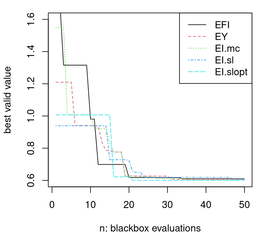
Although they start at different places, because they are seeded with different (random) space-filling designs, they all end up at about the same place after just 25 blackbox evaluations – at what we know from Figure 7.25 to be the global (valid) optimum. That’s pretty impressive considering that ALoptim (§7.3.4) required 332 evaluations, but offered only local convergence. Despite starting from different spots, the curve labeled “EI.slopt” (corresponding to slack=2) is consistently first to get down to a BVV of about 0.6, the global minimum.
The curious reader may wish to wrap those calls in for loops to explore average case behavior. Panels of Figure 7.29, which are based on a similar exercise from Picheny et al. (2016), used 100 random restarts and included several other methods for comparison.
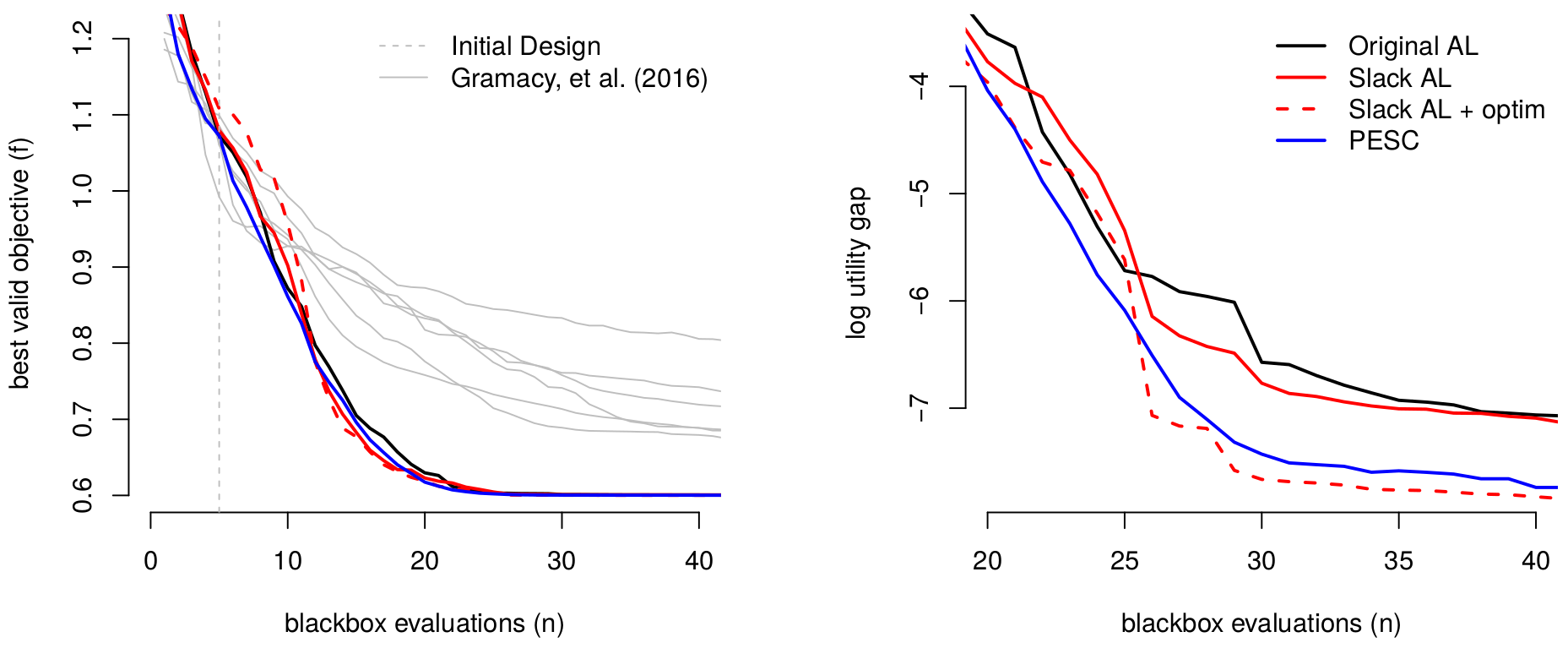
FIGURE 7.29: Cribbed summary of comparison from Picheny et al. (2016) of raw BVV (left) progress, and log utility gap (right) in order to zoom in on the best methods in later iterations.
The left panel shows BVV. All four methods entertained are pretty speedy compared to ordinary, non surrogate-assisted AL, consistently finding the global minimum after 25 blackbox evaluations. The blue comparator, PESC for predictive entropy search (Hernández-Lobato et al. 2015) leverages an implementation in spearmint, a Python library. Comparisons are drawn to methods from Gramacy et al. (2016) in gray: ALBO but without slack variables, automatic initialization (7.13) or single-acquisition (inner loop) termination. Taken together, those engineering details offer a dramatic improvement over the initial prototype.
The right panel shows log utility gap, \(\log(\mathrm{BVV}_n - y^\star)\) over acquisitions \(n=n_0, \dots, N\), tracking log differences between the theoretical BVV of the objective, \(y^\star\), and those found by search (empirical BVV). Under this progress metric, separation between the best comparators is accentuated. Perhaps more notably, all methods continue to make progress well beyond the twenty-fifth evaluation, albeit only incrementally. PESC and slack AL with meta-optimization of EI are best; pairwise \(t\)-tests reveal that these differences are indeed statistically significant. See Picheny et al. (2016) for more details.
Unknown objective
How about if the objective function is more complicated and, along with constraints, expensive to evaluate jointly in the blackbox? Sure. To illustrate, how about augmenting our toy aimprob with the objective below?
herbtooth <- function(X)
 {
  if(!is.matrix(X)) X <- matrix(X, ncol=2)
  g <- function(z)
    return(exp(-(z - 1)^2) + exp(-0.8*(z + 1)^2) - 0.05*sin(8*(z + 0.1)))
  return(-g(X[,1])*g(X[,2]))
 }
Some have been calling this function “Herbie’s tooth” because it was cooked up by Herbie Lee, my PhD advisor, as a challenging surface to model and optimize (H. Lee et al. 2011; Gramacy and Lee 2011). Herbie’s tooth has featured in several recent papers, including the local approximate Gaussian process (LAGP) paper (Gramacy and Apley 2015). When visualized as a perspective plot, as we shall do in Chapter 9’s Figure 9.25 when we get to LAGP, it looks like a molar. A mathematical depiction is provided by Eq. (9.3). Without dense sampling in the input space it’s hard to accurately emulate this test function. More relevant in our current context is that molars have lots of nooks and crannies, i.e., local minima, which makes for a challenging optimization problem.
For visuals, and ultimately to optimize under aimprob constraints, an updated aimprob2 function is defined below, using herbtooth in place of the known linear objective. Herbie’s tooth is usually evaluated in \([-2,2]^2\), whereas observe that aimprob2 assumes coded inputs.
aimprob2 <- function(X, known.only=FALSE)
 {
  if(is.null(nrow(X))) X <- matrix(X, nrow=1)
  if(known.only) stop("no outputs are treated as known")
  f <- herbtooth(4*(X - 0.5))
  c1 <- 1.5 - X[,1] - 2*X[,2] - 0.5*sin(2*pi*(X[,1]^2 - 2*X[,2]))
  c2 <- rowSums(X^2) - 1.5
  return(list(obj=f, c=drop(cbind(c1, c2))))
}
Leveraging our plotting macro from earlier, Figure 7.30 shows the surfaces in play in this updated toy problem. Plainly, there’s a multitude of local minima, in both valid and invalid parts of the input space.
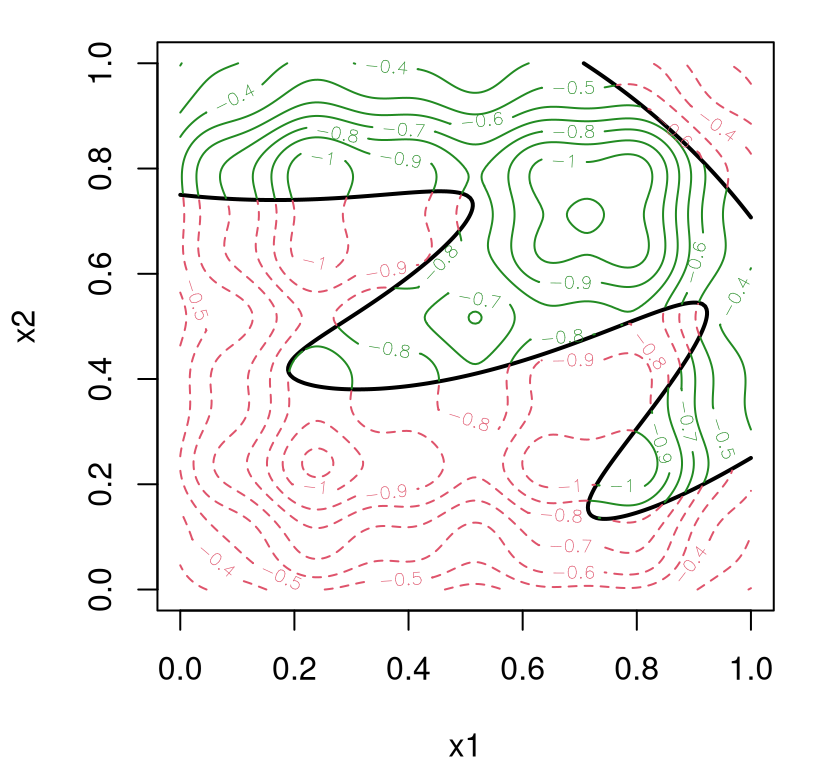
FIGURE 7.30: Herbie’s tooth objective paired with constraints from the original toy problem (7.8).
By inspection, it would appear that there are three local minima which are more-or-less equally good as global optima in three of the four quadrants of the space. A fourth one, located in the remaining quadrant, would be similarly attractive if not invalid. These are, roughly speaking, at combinations of coordinates 0.25 and 0.75 up from zero and down from one. To see how well surrogate AL and MC EI work on this problem, code below performs searches in thirty replicates, averaging over randomized seed designs. Specifying fhat=TRUE causes a GP surrogate to be fit to objective function evaluations returned by blackbox.
prog <- matrix(NA, nrow=30, ncol=100)
xbest <- matrix(NA, nrow=30, ncol=2)
for(r in 1:30) {
  out2 <- optim.auglag(aimprob2, B, fhat=TRUE, start=20, end=100, verb=0)
  prog[r,] <- out2$prog
  v <- apply(out2$C, 1, function(x) { all(x <= 0) })
  X <- out2$X[v,]
  obj <- out2$obj[v]
  xbest[r,] <- X[which.min(obj),]
}
Full BVV progress is recorded over acquisition iterations, as are \(x\)-coordinates corresponding to the best solution found in each replicate. Figure 7.31 shows our thirty progress trajectories over 100 blackbox evaluations.
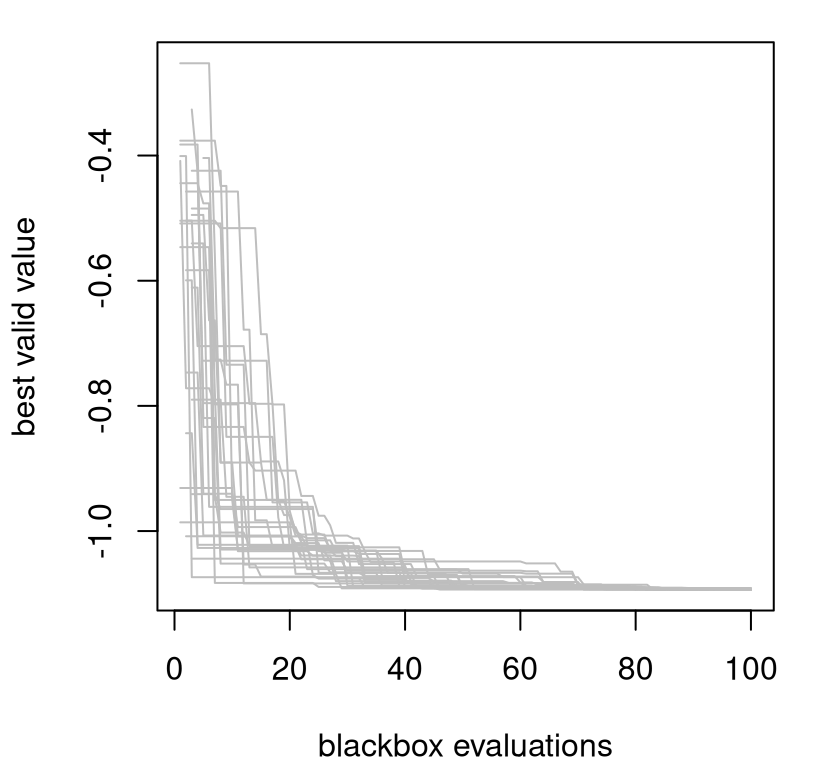
FIGURE 7.31: Best valid value for ALBO search of Herbie’s tooth with toy constraints (7.8) in thirty random restarts.
All searches have converged on an agreed-upon objective evaluation of about -1.0929 for the BVV at the final iteration. Figure 7.32 shows the geographical locations of the valid \(\mathrm{argmin}_x\) found in each restart.
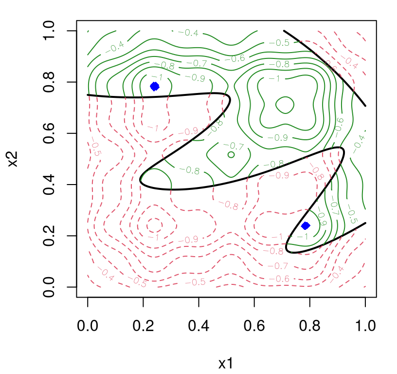
FIGURE 7.32: Locations of solutions \(x^\star\) from each of thirty repetitions.
Apparently, only two of the three local valid minima are reasonable as global solutions. There’s some jitter in solutions found owing to MC approximation of EI on space-filling candidate grids. A more precise solution can be calculated, at substantially greater computational expense, with slack=2. A thriftier option might be to initialize a classical, local AL-based search staring off where the surrogate/EI one ended. For a more compelling illustration, let’s back off the number of blackbox iterations to half of what was used above.
out2 <- optim.auglag(aimprob2, B, fhat=TRUE, start=20, end=40, verb=0)
v <- apply(out2$C, 1, function(x) { all(x <= 0) })
X <- out2$X[v,]
obj <- out2$obj[v]
xbest <- X[which.min(obj),]
Then feed the input corresponding to the BVV, calculated above, into ALoptim. Finishing a surrogate-assisted optimization with a classical one, to drill down a local trough in order to increase precision of the final solution, is a common tactic (e.g., Taddy et al. 2009).
end <- length(out2$rho)
evals <- 0
drill <- ALoptim(aimprob2, B, start=xbest, lambda=out2$lambda[end,],
  rho=out2$rho[end], kmax=1, maxit=100)
evals
## [1] 49The histogram in Figure 7.33 shows how xbest, calculated above from just 40 evaluations, compares to results we obtained earlier after 100 runs. Although that result is clearly sub-optimal, just 49 further evaluations within ALoptim – depending on the Rmarkdown build – yields an answer (drill) that’s at least as good as those using 100.
hist(prog[,100], main="", xlab="best valid value",
  xlim=range(c(prog[,100], min(obj))))
abline(v=min(obj), col=2, lty=2)
abline(v=drill[2,3], col=2)
legend("top", c("xbest", "drill"), col=2, lty=2:1)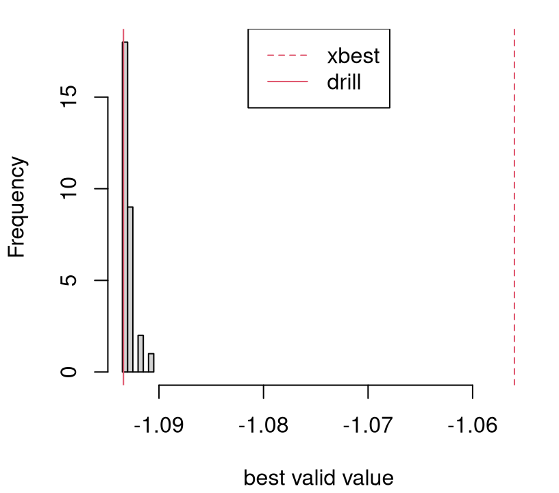
FIGURE 7.33: Histogram of BVVs in thirty repetitions augmented with \(f(x^\star)\) from a limited AL-based search (vertical red-dashed line) followed by ordinary AL-search \(f(x^{\mathrm{drill}})\) initialized at \(x^\star\) (red-solid).
Surrogate-based AL search, via MC EI, finds the local domain of attraction of the global solution in relatively few evaluations. Embarking on a local search from there usually yields an answer that’s indistinguishable from one obtained from a more laborious search enjoying greater global scope, and a more judicious balance between exploration and exploitation.
7.3.8 Equality constraints and more
Several other examples, with comparison to EFI and classic AL, are illustrated by demos provided with the laGP package. For example, demo("ALfhat") duplicates the example immediately above, offering comparison to a classical AL (ALoptim-like) implementation. Two other demos in the package entertain a mixed constraints setting. EFI isn’t directly applicable in the presence of equality constraints; ALBO methods represent the only surrogate-assisted option expressly targeting equality (and mixed) constraints – at least that I’m aware of at the time of writing.
It’s tempting to try transforming an equality constraint into two inequalities (one \(\leq\) and one \(\geq\), or whose negation is \(\leq\)). To the extent that the effect of such a reformulation is understood, the outlook is bleak. It puts double-weight on equalities and violates certain regularity conditions. Numerical issues have been reported in empirical evaluations (Sasena 2002). This EFI-enabling hack is included in empirical comparisons automated by the two demos.
See demo("GSBP") for a 2d problem involving a Goldstein–Price objective (§7.1.1), the toy sinusoidal inequality constraint \(c_1\) from aimprob, and two equality constraints that together trace out four ribbons of valid region. EFI under the dual-inequality transformation is competitive on this problem, but AL methods, especially with slack=2, work better. See demo("LAH") for a 4d problem with known linear objective, an inequality constraint derived from the Ackley function, and an equality constraint derived from the Hartmann 4 function. EFI is pretty bad on this one because the dual inequality transformation over-emphasizes the equality constraint relative to the inequality one.
It would be remiss not to mention that optim.auglag isn’t equipped to handle noisy blackboxes at this time, whether in the objective, constraint or both. An adaptation estimating nuggets would be relatively straightforward. Still, such a setup is untested at this time, and thus potential pitfalls are unknown. A recent paper by Letham et al. (2019) targets noisy constrained optimization under an updated EFI. Calculations therein utilize quasi MC numerics to fully quantify, and thus balance, relevant uncertainties in acquisition of new runs.
Whenever there’s noise, and especially when it’s substantial, balance between exploration and exploitation is nuanced. Understanding what’s signal and what’s noise is essential to knowing whether there’s potential for improvement. Authors in recent literature have been quick to criticize EI-like methods for acquiring replicates, or nearly so, prompting a search for alternative heuristics. Replicating may seem wasteful when the blackbox is expensive, but repeated sampling represents the only fool-proof mechanism for separating signal from noise. It’s similarly wasteful to sample heavily in a region under the belief that the signal shows potential for improvement when a small handful of replicates could summarily dismiss that potential as noise.
I think this setting represents one of the big open problems in BO, especially when noise levels may change over the input region. New sequential design heuristics, surrogate models, and methods for coping with constraints (like the AL) will be needed in this setting. See, for example, Jalali, Van Nieuwenhuyse, and Picheny (2017). Chapter 10 introduces heteroskedastic GPs, illustrating how replication in design is key to effective learning, prediction, and quantification of uncertainty. Learning for optimization is different than learning for prediction, but similar themes are often in play, albeit to varying degrees.
Math programming has owned optimization for a century, or perhaps longer. And they may yet, at least in some generality, for yet a century more. That said, statistical methods have a near monopoly when observations are noisy. Therefore, the landscape of research into methods for BO – as opposed to the more classical math programming option – will undoubtedly be a space to watch for developments targeting optimization under uncertainty. In many such contexts, such as in e-commerce, those methods (particularly the most exciting developments from the ML/BO literature) already make up the vanguard.
As researchers in applied science become more comfortable with simulation as a means of exploring complex relationships in biology, epidemiology, economics, sociology, physics, chemistry, engineering, and more, they will eventually turn to statisticians for help optimizing and calibrating those systems as a means of affecting policy, implementation, design of new systems and modernization of old. Descriptive power, scope for synthesis, and potential for automation inherent in modern nonparametric and hierarchical models (and their experimental design) is unprecedented in modern times. BO is but one fine example of the confluence of these mathematical and technological advances. Sensitivity analysis and calibration are another.
7.4 Homework exercises
These problems explore Bayesian optimization in objective-only and constrained settings.
#1: Thompson sampling and probability of improvement
Augment the running Goldstein–Price example (§7.1.1) to include optim with method="Nelder-Mead", Thompson sampling (TS; §7.1.2) and PI (7.2) comparators. For TS, base acquisitions on a predictive draw obtained on candidates formed randomly in two variations:
- A novel size-100 LHS in the full \([0,1]^2\) input space for each iteration of search.
- A novel size-90 LHS in \([0,1]^2\) augmented with ten candidates selected at random from the smallest rectangle containing the best five inputs found so far.
Considering the similarity between these four new methods and ones presented in the chapter ("L-BFGS-B", EY, EI), you may wish to develop a more modular implementation where code and initializing points can be shared. That investment will pay dividends in #2 and #3 below.
Report average progress and provide boxplots of the best objective value (BOV) for all seven comparators over one hundred repetitions.
#2: Six-dimensional problem
Consider the Hartmann 6 function as implemented by hartman6 in the DiceOptim package (Picheny, Ginsbourger, and Roustant 2016) on CRAN. Re-tool the running Goldstein–Price example (§7.1.1) and EY-v-optim-v-EI comparison for this setting. As in #1, perform up to fifty blackbox evaluations where surrogate-assisted variations are seeded with a random design of size \(n_0 = 12\). Report average progress over optimization acquisitions and provide a boxplot of the BOV for each at the end. If you worked on #1, perhaps include those comparators as well.
#3: Adding noise
Revisit #1 and #2, above, with blackbox evaluations observed with additive noise: \(Y(x) = f(x) + \varepsilon\). Take \(\varepsilon \sim \mathcal{N}(0, \sigma^2 = 0.1^2)\) for both problems. Noise makes the problem harder, and it can help to seed with replicates in order to separate signal from noise. So take \(N=75\) with \(n_0=20\) composed of two replicates on an LHS of size ten. Since "L-BFGS-B" isn’t a reasonable comparator in this context, replace with an optim-based IECI measured on novel size-100 LHS reference sets in each iteration. Report average progress in terms of the true, no-noise output over optimization acquisitions and provide a boxplot of the true BOV for each at the end. If you worked on #1, perhaps include those comparators as well.
#4: EFI versus IECI for optimization under constraints
Treat the function htc below, which returns objective and constraint, as a blackbox.
library(splancs)
htc <- function(X, epoly)
 {
  if(!is.matrix(X)) X <- matrix(X, ncol=2)
  z <- herbtooth(X)
  cl <- rep(1, length(z))
  if(!is.null(epoly)) {
    xy <- as.points(X[,1], X[,2])
    io <- inout(xy, epoly)
    cl[!io] <- 0
  }
  return(list(obj=z, c=as.numeric(!cl)))
 }
Valid region is defined by the polygon epoly, which we shall take to approximate an ellipse.
library(ellipse)
epoly <- ellipse(rbind(c(1,-0.5), c(-0.5,1)), scale=c(0.75, 0.75))
formals(htc)$epoly <- epoly
Work with a pre-defined \(200 \times 200\) grid in \([-2,2]^2\). Starting with \(n_0 = 25\) random grid-points, find the best valid value (BVV) of the objective (on that grid) in a budget of 50 further evaluations, for \(N=75\) total, in the following variations. Hint: you may wish to plot objective and constraint surfaces on a grid first to see what you’re dealing with.
- Use a GP surrogate for the objective, and a random forest (RF) surrogate (via
randomForest) for the constraint. Base acquisitions on EFI over remaining candidates from the grid. - Similarly with GP for the objective and RF for the constraint, base acquisitions on IECI over remaining candidates from the grid, taking as reference locations 100 novel random candidates. (A reference set of 1000 would be even better, if you can afford the computation.)
While you’re gathering those acquisitions, keep track of the truly best valid value. That is, among the grid elements which are actually valid, ignoring the RF classifier, save the objective value of the grid location which your model predicts is lowest. Also save the entire cache of \(x\), and \((y, c)\)-evaluations collected over the fifty acquisitions. Repeat the experiment fifty times and report visually, and comment verbally, on patterns in these summaries of performance.
Finally, explore demo("plconstgp_2d_ieci") in plgp on CRAN which couples a regression GP for the objective with a classification GP for the constraints in a fully Bayesian setup (Gramacy and Lee 2011). Compare and contrast performance against your implementation. (Note there’s no grid in the demo.)
#5: An old friend
Revisit exercise #3 from §1.4, which combined the Goldstein–Price function as an objective, with the sinusoidal constraint from aimprob (7.8), via EFI (optim.efi) and augmented Lagrangian (optim.auglag) support provided by laGP. For the AL, try both EY (ey.tol=1) and EI, the default, with and without slack variables. Use arguments start=10 and end=60 for a total of fifty acquisitions after initializing with a small LHS of size ten. How do your new results compare to the mathematical programming approach you took earlier? Considering the random nature of initialization(s), you may wish to average over thirty or so runs in order to explore variability. Track BVV of the objective over the iterations, reporting its average over the repetitions and full distribution after the last acquisition. Hint: this exercise is a simplified version of what you would find as demo("GSBP") in laGP.
#6: Remediation by optimization
Revisit the Lockwood solvent groundwater plume site case study from §2.4. The program described therein is reproduced below. With \(x_j\) denoting the pumping rate for well \(j\), solve
\[ \min_{x} \; \left\{f(x) = \sum_{j=1}^6 x_j : c_1(x)\leq 0, \, c_2(x)\leq 0, \, x\in [0, 2\cdot 10^4]^6 \right\}. \]
If you’ve not done so already, see exercise #4a from §2.6 in order to compile and test the runlock back-end.
Your task is to perform up to 500 iterations of optimization under each of EFI, IECI and the augmented Lagrangian (AL) with EY and EI alternatives.
- For AL variations use
optim.auglagfromlaGPwith the following recommended settings.- Work with coded inputs by providing
Bscale=10000and use bounding boxB=matrix(c(rep(0,6), rep(2,6)), ncol=2). - Use a separable covariance specification with
sep=TRUE. - You may also find it helpful, but slower, to use
ncandf=function(t) { 1000 }rather than the default search candidate setting. - For EY rather than EI, specify
ey.tol=1.
- Work with coded inputs by providing
- For EFI use
optim.efiinlaGP.- Same suggestions as above for
optim.auglagapply here.
- Same suggestions as above for
- For for IECI you’ll have to do it yourself, but you may use the GP fitting capability built into
laGP.- Note that
ieciGPsepmodels the objective \(f\), whereas our objective, above, is a known linear function. - Describe how it could be modified to accommodate the known objective. A description is sufficient; you don’t need to actually do it (because the setup will still work, but perhaps not as efficiently).
- Note that
- On all of the above, you might find it helpful to try an easier, less expensive blackbox where you know the answer, like in #4 or #5, first.
Compare your BVV progress to results from the Matott, Leung, and Sim (2011) study, which you can find in runlock/pato_results.csv.
- In each case, initialize your search with 30 space-filling candidates (e.g.,
start=30inoptim.*). - Optionally, use
Xstartto seed those comparators with identical initial designs, which could help facilitate a lower variance comparison. - Put a
forloop around your optimizations and report average BVV progress over as many random restarts as you have time for (or you think are sufficient to stamp out MC error).
References
randomForest: Breiman and Cutler’s Random Forests for Classification and Regression. https://CRAN.R-project.org/package=randomForest.
CompQuadForm: Distribution Function of Quadratic Forms in Normal Variables. https://CRAN.R-project.org/package=CompQuadForm.
plgp: Particle Learning of Gaussian Processes. https://CRAN.R-project.org/package=plgp.
laGP: Local Approximate Gaussian Process Regression. http://bobby.gramacy.com/r_packages/laGP.
sadists: Some Additional Distributions. https://CRAN.R-project.org/package=sadists.
DiceOptim: Kriging-Based Optimization for Computer Experiments. https://CRAN.R-project.org/package=DiceOptim.
Here I’m re-purposing \(m\), previously notating dimension of the input space where \(x\) lives, for the number of constraints. None of the discussion in this chapter demands clarity on input dimension, relieving potential for ambiguity.↩︎