B An Experiment Game
In-class games are a fun way to engage students in difficult and seemingly esoteric material (H. K. H. Lee 2007). Out-of-class games, played over an entire semester say, are less common but can effectively synthesize real-life settings such as those encountered in response surface methodology (RSM; Chapter 3) and Bayesian optimization (BO; Chapter 7). One such game was proposed, and first played over forty years ago (Mead and Freeman 1973). Today, few are aware of that contribution in spite of a citation featuring prominently in a canonical RSM text (Box and Draper 2007). Perhaps this is because Mead and Freeman were ahead of their time. Their setup required a computing environment with student access, and so on, decades before ubiquitous desktop and laptop computing. Today with R, Rmarkdown and shiny (Chang et al. 2017) web interfaces, barriers have come way down.
B.1 A shiny update to an old game
Mead and Freeman’s original game centered around blackbox evaluation of agricultural yield as a function of six nutrient levels, following a form borrowed from Nelder (1966):
yield <- function(N, P, K, Na, Ca, Mg)
 {
  l1 <- 0.015 + 0.0005*N + 0.001*P + 1/((N+5)*(P+2)) + 0.001*K + 0.1/(K+2)
  l2 <- 0.001*((2 + K + 0.5*Na)/(Ca+1)) + 0.004*((Ca+1)/(2 + K + 0.5*Na))
  l3 <- 0.02/(Mg+1)
  return(1/(l1 + l2 + l3))
 }
Players were asked to supply settings for inputs across five campaigns, simulating crop years. In each campaign, after observing yield under a Gaussian noise regime determined by additive block and plot-within-block effects, players could use data to update fits and revise strategies for future campaigns. The ultimate goal was to maximize yield, primarily with Chapter 3-like tools such as steepest ascent and ridge analysis. In a modern landscape of computer experiments, the Mead and Freeman (1973) game seems somewhat antiquated, harking back to Fisher’s 1920s work at Rothamsted Experimental Station.
Gramacy (2018a, hereafter “I”) described a revised variation motivated by modern technology/application, and a more sophisticated methodological toolkit, such as for BO in Chapter 7. Other enhancements target friendly competition through leaderboards and benchmarks, carrots to encourage regular engagement, and partial solutions to catch-up straggling students. Perhaps the biggest innovation in this reboot is the use of modern web interfaces. Game play is facilitated by an R shiny app, shown in Figure B.1, which serves as both a multi-player portal and an interface to the back-end database of player(s) records. Code supporting the app is linked from the book web page.
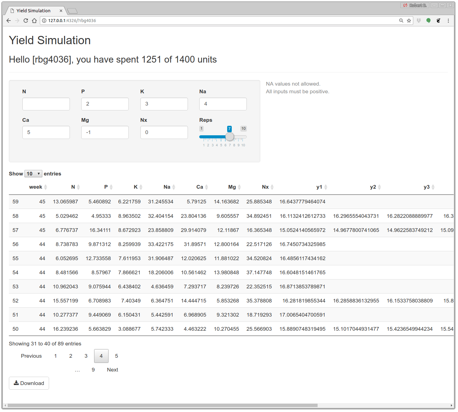
FIGURE B.1: Interactive yield simulation session. Duplicated from Gramacy (2018a).
Once logged in, the player is presented with three blocks of game content. Players are identified by their initials, as in the leaderboard discussed in §B.2, and a secret four-digit pin. The view in the figure is for my personal session; my initials are “rbg” and I chose my office number “403G” as a pin. A greeting block at the top of the page in the figure provides details on my spent and total budget for experimental runs. Details on how budget replenishes weekly, and how a schedule of run costs encourages including replication in the design of runs (§10.3.2), are left to Section 2.2 of Gramacy (2018a). As long as the player has not over-spent their budget, new runs may be performed by entering coordinates and a number of replicates into the second block on the page shown in the figure. Once all entries are valid, a “Run” button appears alongside a warning that there are no do-overs.
Performing a run causes the table in the final block of the page to be updated. All together, the table has 18 columns, recording run week, 7 input coordinates, and up to ten outputs. It’s primary purpose is visual confirmation that new runs have been successfully incorporated into the player’s database file. It’s not intended as the main data-access vehicle. A “Download” button at the bottom saves a text-formatted table to the player’s ~/Downloads directory.
One modern twist in the game’s construction encourages players to think about signal-to-noise trade-offs, and nudges them to spend units regularly rather than save them all until the final week of game play. I was worried that students would procrastinate, and wanted to devise a scheme that encouraged rather than mandated engagement. So variance of the additive noise on yield simulations changes weekly, following a smooth process in time. Starting in week \(w_s\), noise in week \(w\) follows
\[ \sigma^2(w) = 0.1 + 0.05 (\cos(2\pi(w - w_s)/10)+1). \]
Noise peaks in this setup during the first and tenth weeks, although players are warned that variance may be monotonically increasing, substantially devaluing late semester binges. A second modern innovation involves the introduction of a seventh input, Nx, that is deliberately unrelated to the response.
Game setup is optimized for play during a fifteen-week semester. I played the game with the class during the Fall semester of 2016. Although the main goal is to optimize yield, a final project assignment prompted students to think about ancillary goals such as main effects (§8.2.2) and sensitivity indices (§8.2.3), and asked them to report on how variance evolves over time (§10.2). Homework exercises encouraged students to try certain specific methods, and were timed with lecture material: beginning with steepest ascent and ridge analysis (Chapter 3) and culminating in BO (Chapter 8). Details and more specific pointers are provided in Gramacy (2018a); all materials are linked from the book web page.
B.2 Benchmarking play in real-time
Among those materials is an Rmarkdown script compiling four “leaderboard” style views into student performance over the weeks of game play. Students could visit the leaderboard any time. It was hosted along with the game interface (Figure B.1) on shinyapps.io. I hoped that friendly competition would spur interest. As a peek into one of the four views provided, code below recreates (de-noised) maximum yield progress over thirteen weeks of game play.
Text files storing each player’s database of runs may be read in as follows.
##  [1] "ame4794.txt" "fs0930.txt"  "hm1113.txt"  "ic2997.txt"
##  [5] "jbl1003.txt" "jh0702.txt"  "jtf1020.txt" "mds6266.txt"
##  [9] "rbg4036.txt" "ss0720.txt"  "wt4512.txt"  "ww2222.txt"
Names of the files concatenate player initials and pins. Each records a table of inputs and noisy outputs, so these inputs must be run back through yield for a de-noised view. De-noising helps identify the true ranking of players, rather than ones corrupted by spurious noise. The function below vectorizes yield in order to streamline that de-noising process. Notice that the seventh, Nx input isn’t used.
Next, code below loops over each player’s database file, building up a data.frame of best results by week. The game was run during weeks 38–51 in 2016, and these results were captured during the final, \(51^{\mathrm{st}}\) week.
wk <- 51
start.wk <- 38
weeks <- (start.wk-1):wk
Ybest <- matrix(-Inf, nrow=length(weeks), ncol=length(files))
for(i in 1:length(files)) {
  data <- read.table(paste0("yield/leaderboard/", files[i]), header=TRUE)
  wk <- data[,1]
  xs <- data[,2:8]
  for(j in 1:length(weeks)) {
    wi <- wk == weeks[j]
    if(j > 1) Ybest[j,i] <- Ybest[j-1,i]
    if(sum(wi) == 0) next
    ybnew <- max(as.matrix(yield.fn(xs[wi,-7])), na.rm=TRUE)
    if(j == 1 || Ybest[j-1,i] < ybnew) Ybest[j,i] <- ybnew
  }
}
In order to mask true outputs, lest players learn the actual (non-noisy) value of their best response over the weeks, visuals of de-noised yields were provided on a normalized scale.
Finally, player pin information is scrubbed to leave only initials for presentation in the legend of the leaderboard.
Figure B.2 shows the result. On the \(x\)-axis is the week of game play, and on the \(y\)-axis is normalized yield. Each player has a line in the plot.
matplot(weeks-start.wk+1, Ybest, type="l", ylab="max yield", xlab="week",
  col=1:length(initials), lty=1:length(initials), lwd=2, xlim=c(0, 19))
legend("bottomright", initials, col=1:length(initials),
  lty=1:length(initials), lwd=2)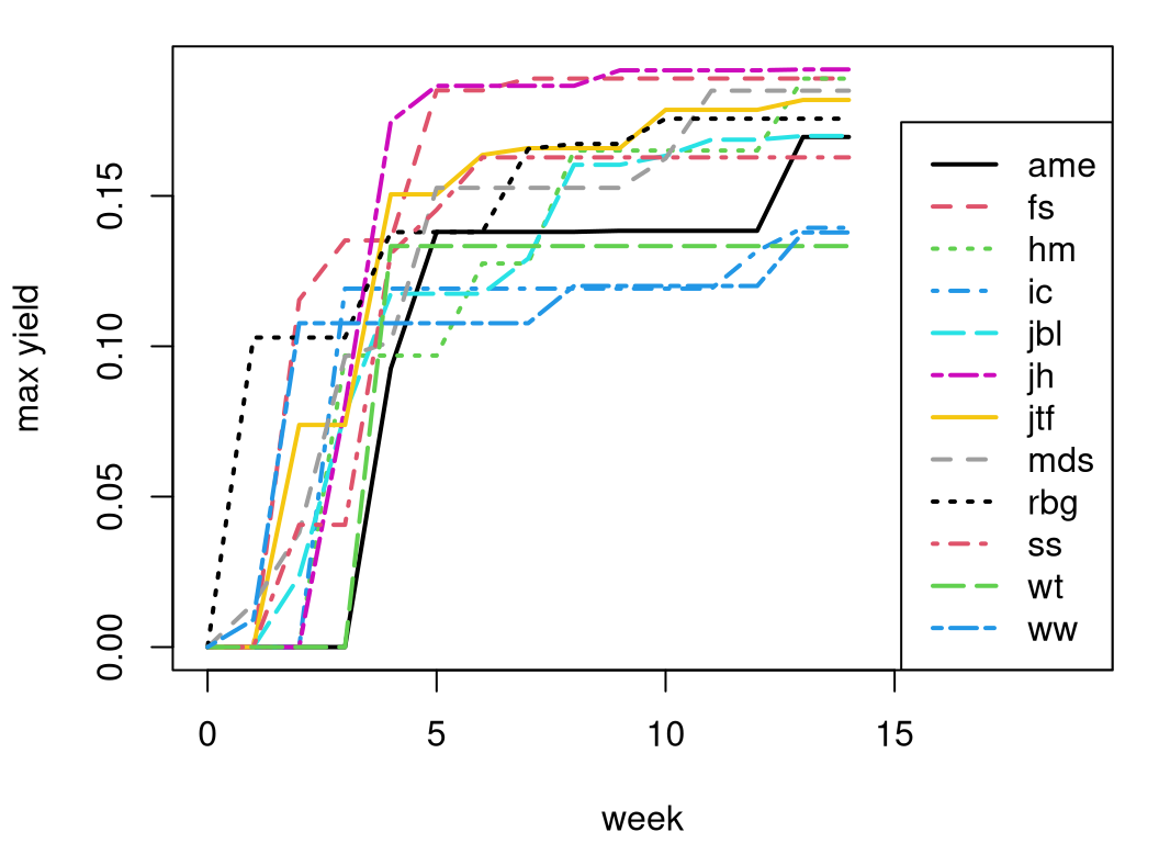
FIGURE B.2: De-noised view into real-time progress on yield optimization captured during the final week of game play.
Observe from the figure that about half of all players’ progress is made in the first five weeks, spanning around forty runs. This is a testament to the prowess of simple, classical RSM from Chapter 3. Most subsequent refinement transpired using more modern, Chapter 7 techniques. Students “jh” and “fs” made rapid progress, whereas “hm” ends up at the same place in the end, but with more steady increments. My own progress (“rbg”) placed me fifth by this measure. I favored replication over unique runs in hopes of obtaining better main effects, sensitivity indices, and estimates of variance over time.
Three other views are provided by the Rmarkdown file leader.Rmd residing in an archive linked from the book web page. One is similar to Figure B.2, presenting de-noised best results over run number instead of by week. Since some students performed many more unique runs than others who favored heavier replication, this view is harder to interpret. Two others present the analog of the first two but without de-noising, and back on the original un-normalized scale.
References
shiny: Web Application Framework for R. https://CRAN.R-project.org/package=shiny.