Chapter 3 Steepest Ascent and Ridge Analysis

This chapter offers a fly-by of classical methods for response surfaces, focusing on local linear modeling. Development closely follows Chapters 5-6 of Myers, Montgomery, and Anderson–Cook (2016), however with rather less on design and greater emphasis on implementation in R. Some of the examples/data are taken verbatim, although with less back-story. Readers who are keen on a more in-depth treatment of the subjects in this chapter will find the Myers text far more satisfying. Of course neither treatment is complete. There are a wealth of texts and modern surveys on the topic.

The goal here is to offer some historical context, in order to facilitate comparisons and contrasts to more modern methodology introduced in subsequent chapters. That said, the methods herein are far better understood, and more widely deployed in practice, particularly in industrial settings. One can argue that they offer more control and potential for insight to the experienced modeler, who deeply understands potential limitations and pitfalls. However, as will become clear as topics progress, many rigid assumptions are embedded in this framework, primarily for analytical tractability. These may be difficult to justify in practice, especially in settings where the goal is to produce an autonomous framework that can operate without constant (expert) human oversight.

What is this chapter about, more specifically? At a high level it’s about collecting and learning from data. Since that’s perhaps too generic, a better question entails not what but why. One reason for data collection and modeling is to develop understanding or to make predictions under novel conditions. Such understanding and predictions could facilitate many aims. But sometimes that’s too ambitious, especially when experimentation (obtaining the “runs” that make up the data) is expensive, and it usually is, or when the ideal modeling apparatus is data hungry. A more humble goal is to make things a little better, which may require less data and where cruder models may be sufficient. That’s what this chapter is about. We’ll return to bigger models and bigger data in subsequent chapters.

The choice of data – the experimental design – and models is supremely important. The two are intimately linked. Yet simple choices work well when focused locally in the input domain, appealing to Taylor’s theorem from calculus. Tools outlined in this chapter are canonical in process optimization or process improvement. Although the goal is to find a configuration of inputs providing a point of optimum response, one more pragmatically settles for simply making an improvement on a previously utilized input setting. Imagine a manufacturing process whose current operating conditions are good, but could potentially be better. Some data could be collected nearby the current regime which, through model fitting and analysis, leads to a potentially new operating regime that may be more efficient. Then the process might iterate, potentially leading to even greater efficiencies, if experimental budgets allow.

The underlying methodology deployed in each iteration is compartmentalized by whether a first-order or second-order model is being entertained. First-order methods fall under the heading of steepest ascent, and these are rather straightforward to anyone with experience in statistical modeling and optimization. Second-order methods are more involved owing to the many shapes a second-order surface can take on (see, e.g., §1.1.2), leading to so-called ridge analysis. Here decisions about how to refine or improve the experiment are nuanced, leaning on careful analysis of standard errors of coefficients whose values determine the nature of the surface (local maxima, rising ridge, saddle, etc.) and thereby what to do in the next stage. Both steepest ascent and ridge analysis compartments share an intimate relationship with experimental design and benefit from a human-in-the-loop throughout stages of iterative refinement. That’s in stark contrast to Bayesian optimization (BO) methods (Chapter 7) which are rather more hands-off, intended for autonomous/automatic implementation.

3.1 Path of steepest ascent

Our presentation here privileges maximization of input–output relationships – in keeping with classical RSM tradition – as measured by data collected on a certain process. Adaptations for minimization, which is more common in modern BO settings, are straightforward. Emphasis is more on modeling and decision making and less on appropriate choices of design. For more details on design(s) such as orthogonal, factorial or central composite design, see Myers, Montgomery, and Anderson–Cook (2016). Throughout we shall work with coded variables, unless otherwise prefaced, and assume designs centered at \(x_j = 0\) in \([-1,+1]\), for \(j=1, \dots, m\). Some designs, such as those named above, would have \(x_j\) take on only these values \(\{-1,0,1\}\). Finally, we presume to be working in a highly localized subset of the input domain on the natural scale, perhaps centering around a setting of inputs representing current operating conditions on which we plan to improve.

The method of steepest ascent involves a first-order model, sometimes fitted with interactions. Predictive equations emitted from a fitted first-order model depend upon estimated regression coefficients \(\hat{\beta}_j \equiv b_j\). Therefore, ignoring their standard errors \(s_{b_j}\) for the moment (see §3.2.3), it’s perhaps not surprising that coordinates along the path of steepest ascent depend on those values. Coordinate directions are determined by the sign of \(b_j\); step sizes depend proportionally on their magnitude \(|b_j|\).

3.1.1 Signs and magnitudes

To begin with an example, suppose an experiment in two input variables produces the following fitted first-order model. So we’re skipping design and fitting stages here and going right to equations defining fitted values and predictive means.

\[\begin{equation} \hat{y} = 20 + 3 x_1 - 1.5 x_2 \tag{3.1} \end{equation}\]

In R:

first.order <- function(x1, x2)
 {
  20 + 3*x1 - 1.5*x2
 }

Signs and magnitudes of estimated coefficients, \(b_1 = 3\) and \(b_2 = -1.5\), determine the path of steepest ascent and result in \(x_1\) moving in a positive direction, twice as fast as \(x_2\) moving in a negative direction. Evaluating first.order as yhat (\(\hat{y}\)) over a grid x1 \(\times\) x2 in the input space …

x1 <- x2 <- seq(-2, 3.5, length=1000)
g <- expand.grid(x1, x2)
yhat <- matrix(first.order(g[,1], g[,2]), ncol=length(x2))
D <- rbind(c(-1,-1), c(-1,1), c(1,-1), c(1,1))

… facilitates the graphical depiction provided in Figure 3.1: contours of yhat values overlayed on a heat plot. Hypothetical design locations are shown as filled dots outlining a square in the input space.

cols <- heat.colors(128)
image(x1, x2, yhat, col=cols)
contour(x1, x2, yhat, add=TRUE)
points(D, pch=19)
points(0, 0)
arrows(0, 0, 3, -1.5)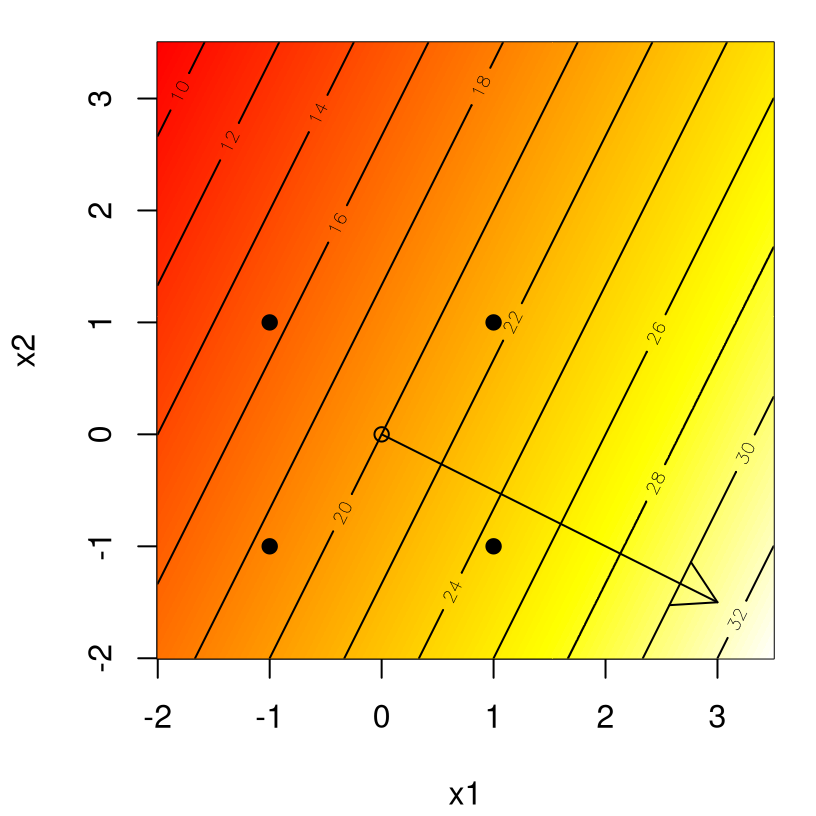

FIGURE 3.1: Example first-order response surface and direction of steepest ascent.

The arrow in the figure, emitting from the center of the design at \((0,0)\), gets its slope from \((b_1, b_2)\). Theoretically the arrow, outlining the path of steepest ascent, runs perpendicular to the contours. However peculiarities in Rmarkdown’s handling of graphical device specifications can introduce skew. If we’re careful, acknowledging that the fitted surface isn’t a perfect representation of the actual surface (presumably getting worse away from the design center), and take baby steps along the path, we may expect to find inputs that improve upon the actual output of the system. So an important question is: how far to explore along the path?

Backing up a bit from the example, let’s now examine the setup more generically in order to formally establish the basic calculations involved in the method of steepest ascent. Consider the fitted first-order regression model

\[ \hat{y}(x) = b_0 + b_1 x_1 + b_2 x_2 + \cdots + b_m x_m. \]

The path of steepest ascent is one which produces a maximum estimated response, with the constraint that all coordinates are a fixed distance, say radius \(r\), away from the center of the design. That definition is captured mathematically by the program

\[ \max_x \hat{y}(x) \quad \mbox{ subject to } \quad \sum_{j=1}^m x_j^2 = r^2. \]

The constraint serves two purposes. One: it’s clearly folly to venture too far away from the origin of the original design, as the fitted surface can only be trusted nearby. Two: in this first-order linear formulation the unconstrained fitted surface is maximized out at infinity, which is an impractical input setting for most purposes.

Solving this optimization problem proceeds by straightforward application of Lagrange multipliers.

\[ L = b_0 + b_1 x_1 + b_2 x_2 + \cdots + b_m x_m - \lambda \left(\sum_{j=1}^m x_j^2 - r^2 \right) \]

Differentiating and setting to zero leads to specifications for each \(x_j\) on the path of steepest ascent,

\[ x_j = \frac{b_j}{2\lambda} \equiv \rho b_j, \quad \mbox{ where } \quad \rho = \frac{1}{2\lambda} \]

may be viewed as a constant of proportionality. For ascent, our default, \(\rho\) is positive; for descent it’s negative. The parameter \(\rho\), which is related to \(\lambda\) and thus to radius \(r\), determines the distance from the design center where the resulting (new) point would reside, which ultimately must be specified by the practitioner.

Extending Figure 3.1, Figure 3.2 shows two potential radiuses \(r_1 = 1\) and \(r_2 = 1.75\) as circles in the plane.

image(x1, x2, yhat, col=cols)
contour(x1, x2, yhat, add=TRUE)
points(D, pch=19)
points(0, 0)
arrows(0, 0, 3, -1.5)
library(plotrix)
draw.circle(0, 0, 1)
text(1, 0, "r1")
draw.circle(0, 0, 1.75)
text(1.75, 0, "r2 > r1")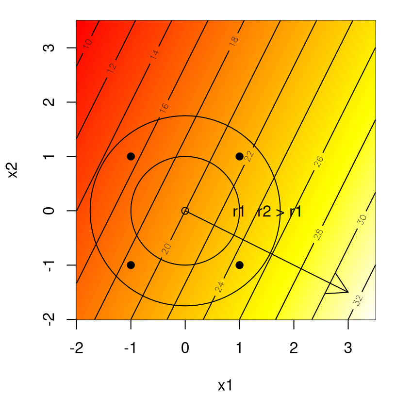

FIGURE 3.2: Radii along paths of steepest ascent.

Input coordinates of new runs can be determined by the intersection between the circle(s) and the path, depicted by the arrow. That enterprise is more simply carried out via choice of \(\rho\) and estimated coefficients \(b_j\). An example follows.

Example: plasma etch process

Plasma etching is a process involved in the fabrication of integrated circuits where a high-speed stream of plasma, the source of which is called an etch species, is shot at a sample. Here we’re interested in etch rate, our response, measured in units of Å/min, as a function of two inputs describing the process: anode-cathode gap (\(\xi_1\)), with natural units of centimeters, and the power applied to the cathode (\(\xi_2\)) in watts. The data in plasma.txt, quoted in Table 3.1, are derived from a \(2^2\) factorial design with four center points.

plasma <- read.table("plasma.txt", header=TRUE)
kable(plasma, caption="Plasma etching data.")

TABLE 3.1: Plasma etching data.

gap	power	x1	x2	etch
1.2	275	-1	-1	775
1.6	275	1	-1	670
1.2	325	-1	1	890
1.6	325	1	1	730
1.4	300	0	0	745
1.4	300	0	0	760
1.4	300	0	0	780
1.4	300	0	0	720

Observe that the data file contains both natural and coded inputs. We wish to move to a region of the input space where etch rate is increased. A goal of the experiment from which these data were derived was to move to a region where etch rate is close to 1000 Å/min. Begin by fitting a first-order model. The code below, with summary.lm output in Table 3.2, first tries a variation with interactions, mostly with the aim of illustrating that the interaction term is unnecessary.

fit.int <- lm(etch ~ x1*x2, data=plasma)
s <- summary(fit.int)$coefficients
kable(s, caption="Summary of first-order model fit with interactions.")

TABLE 3.2: Summary of first-order model fit with interactions.

	Estimate	Std. Error	t value	Pr(>|t|)
(Intercept)	758.75	8.604	88.189	0.0000
x1	-66.25	12.168	-5.445	0.0055
x2	43.75	12.168	3.596	0.0228
x1:x2	-13.75	12.168	-1.130	0.3216

Since the x1:x2 coefficient isn’t statistically significant, re-fit with an ordinary first-order model as follows …

fit <- lm(etch ~ x1 + x2, data=plasma)
coef(fit)

## (Intercept)          x1          x2 
##      758.75      -66.25       43.75

… yielding the following fit which we shall use as the basis for constructing a path of steepest ascent.

\[ \hat{y} = 758.75 - 66.25 x_1 + 43.75 x_2 \]

The sign of \(x_1\) is negative and the sign of \(x_2\) is positive, so we shall seek improvements in etch rate by decreasing gap and increasing power. For every unit change in gap (\(x_1\)), the corresponding change in power (\(x_2\)) may be calculated as follows.

b1 <- coef(fit)[2]
b2 <- coef(fit)[3]
delta2 <- abs(b2/b1)
delta2

##     x2 
## 0.6604

If we choose the gap step size (in coded units) to be \(\Delta x_1 = -1\), then the power step size is delta2 \(=\) 0.6604. All right, let’s consider three potential new runs along that path with \(\Delta x_1 \in \{-1, -2, -3\}\), stored in an R data.frame as follows.

Dnew <- data.frame(x1=(-1):(-3), x2=(1:3)*delta2)

To aid in visualization, code below first evaluates the fitted model, through its predictive equations, on a grid for image/contour plotting.

x1 <- seq(-4, 1.5, length=100)
x2 <- seq(-1.5, 4*delta2, length=100)
g <- expand.grid(x1=x1, x2=x2)
yhat <- matrix(predict(fit, newdata=g), ncol=length(x2))

Figure 3.3 shows that surface, again via contours overlayed on a heat plot and design indicated as filled dots. An arrow outlines the path of steepest ascent, and three open circles along that path are derived from Dnew, calculated above.

image(x1, x2, yhat, col=cols)
contour(x1, x2, yhat, add=TRUE)
points(plasma$x1, plasma$x2, pch=19)
points(0, 0)
arrows(0, 0, -3.5, 3.5*delta2)
points(Dnew)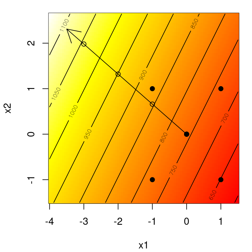

FIGURE 3.3: Steps along the path of steepest ascent for plasma etch data.

Steepest ascent path in hand, including particular input settings, the next step is to perform new runs at those settings. Doing that requires inputs in natural units, which can be derived one point at a time or for the path at large. The latter in our case is \((\Delta \mathrm{gap}, \Delta \mathrm{power}) = (-0.2 \mathrm{cm}, 16.5 W)\), and the file plasma_delta.txt contains inputs and responses for three runs along this path, i.e., via \(\Delta = \{1,2,3\}\). These are shown in Table 3.3.

plasma.delta <- read.table("plasma_delta.txt", header=TRUE)
plasma.delta$p.etch <- predict(fit, newdata=plasma.delta[,4:5])
kable(plasma.delta, 
  caption="Plasma observations along the path of steepest ascent.")

TABLE 3.3: Plasma observations along the path of steepest ascent.

Delta	gap	power	x1	x2	etch	p.etch
1	1.2	316.5	-1	0.66	845	853.9
2	1.0	333.0	-2	1.32	950	949.0
3	0.8	349.5	-3	1.98	1040	1044.1

In the jargon, the first run, corresponding to \(\Delta = 1\), is called a confirmation test. It’s reassuring to observe that the output (about 845) is close to our prediction (854). This output, assuming we haven’t seen/performed the other two runs yet, suggests we’re moving in the right direction. However, 845 and 854 are not better than the best run on our original design.

max(plasma$etch)

## [1] 890

Therefore it stands to reason (with caution) that we could go a little farther along the path of steepest ascent and expect further gains. Indeed that is the case, and again our predicted and observed outputs farther along the path are in remarkable agreement. The response from the last run, corresponding to \(\Delta = 3\), indicates that the experimental objective of an etch rate of 1000 Å/min has been met. Note that the actual etch response (1040) is slightly lower than our predicted one (1044.125).

Considering our success, it might be tempting to explore farther along the path. Actually, the conventional wisdom here – once substantially outside the original experimental region – would be to re-design an experiment centered at the new best value in order to allow for a potential mid-course correction, i.e., to better align the estimated and actual path of steepest ascent. Before turning to another, bigger example, let’s take a moment to codify the method in terms of an easy-to-find (and follow) algorithm, say for help on homework exercises (§3.3). The description in Algorithm 3.1 is liberally cribbed from Myers, Montgomery, and Anderson–Cook (2016).

Algorithm 3.1: Steepest Ascent for First-Order Models

Assume that the point \(x_1 = x_2 = \cdots = x_m = 0\) is the base or origin point.

Require fitted first-order model with coefficients \(b_1, \dots, b_m\).

Then

1. Choose a reference variable index \(j \in \{1, \dots, m\}\). It doesn’t matter which; common choices include:
   1. the variable with the largest absolute coefficient \(|b_j|\), possibly adjusted by standard error \(|b_j|/s_{b_j}\);
   2. the input most familiar to the practitioner;
   3. the variable with the widest (relative) range as measured in natural units.
2. Choose a step size \(\Delta x_j\) in coded units.
3. Calculate the step size in the other variables relative to \(x_j\).

\[ \Delta x_k = \frac{b_k}{b_j/\Delta x_j}, \quad k \ne j \]

Return \(\Delta x_k\), for \(k=1,\dots,m\), possibly after first mapping from coded back to natural variables.

A bigger example: shrinkage

To accommodate for shrinkage in injection-molding processes it’s common for dies for parts to be built larger than their nominal, or desired size. In order to minimize the amount of shrinkage for a particular part, an experiment was conducted varying four factors known to impact shrinkage. The experiment consisted of an un-replicated \(2^4\) factorial design using the factors outlined in Table 3.4.

TABLE 3.4: Mapping of shrinkage inputs.

Factor	Name (natural units)	-1	+1
\(x_1\)	Injection velocity (ft/sec)	1.0	2.0
\(x_2\)	Mold temperature (°C)	100	150
\(x_3\)	Mold pressure (psi)	500	1000
\(x_4\)	Back pressure (psi)	75	120

Let’s extract those ranges as an R matrix so that they may be used by the implementation to follow.

r <- cbind(c(1,2), c(100, 150), c(500,1000), c(75,120))
colnames(r) <- c("vel", "temp", "mpress", "bpress")

The center of the space, representing our baseline setting, is …

base <- r[1,] + (r[2,] - r[1,])/2
base

##    vel   temp mpress bpress 
##    1.5  125.0  750.0   97.5

… in natural units. This corresponds to the zero vector on the coded scale. Unfortunately we don’t have access to the actual observed responses (which are measured in units of \(10^{-4}\) as deviations from nominal) at each input combination, but we do have a first-order model fit to that data (in coded units):

\[ \hat{y} = 80 - 5.28 x_1 - 6.22 x_2 - 1.21 x_3 - 1.07 x_4. \]

Following Step 1 in Algorithm 3.1, suppose that we were to select \(x_1\) as the reference variable defining the step size. In Step 2 choose \(\Delta x_1 = 1\), corresponding to a 0.5 ft/sec injection velocity. Then, relative to that choice we have the following adjustments \(\Delta\).

b <- c(-5.28, -6.22, -1.21, -1.07) 
delta <- b/b[1]
delta

## [1] 1.0000 1.1780 0.2292 0.2027

R code below gathers input settings, collected into a data.frame, along the path of steepest descent up to \(4 \Delta\) in coded units.

path <- rbind(0, 
  apply(matrix(rep(delta, 4), ncol=4, byrow=TRUE), 2, cumsum))
colnames(path) <- paste0("x", 1:4)
rownames(path) <- paste0("Base +", 0:4, "Δ")

Before displaying coordinates on the path, let’s convert to natural units. The corresponding changes on that scale are …

dnat <- delta*(r[2,] - r[1,])/2
dnat

##    vel   temp mpress bpress 
##   0.50  29.45  57.29   4.56

… augmenting our data.frame as shown in Table 3.5.

pnat <- rbind(base, matrix(rep(base, 4), ncol=4, byrow=TRUE) + 
  apply(matrix(rep(dnat, 4), ncol=4, byrow=TRUE), 2, cumsum))
colnames(pnat) <- c("ft/sec", "°C", "psi", "psi")
rownames(pnat) <- rownames(path)
kable(cbind(path, pnat), digits=5, 
  caption="Steps along path of steepest ascent for shrinkage example.")

TABLE 3.5: Steps along path of steepest ascent for shrinkage example.

	x1	x2	x3	x4	ft/sec	°C	psi	psi
Base +0Δ	0	0.000	0.0000	0.0000	1.5	125.0	750.0	97.5
Base +1Δ	1	1.178	0.2292	0.2026	2.0	154.5	807.3	102.1
Base +2Δ	2	2.356	0.4583	0.4053	2.5	183.9	864.6	106.6
Base +3Δ	3	3.534	0.6875	0.6079	3.0	213.4	921.9	111.2
Base +4Δ	4	4.712	0.9167	0.8106	3.5	242.8	979.2	115.7

Then it’s simply a matter of convincing whomever manages the process to tinker with settings along that schedule. Sometimes that’s easier said than done. It could help to give them an inkling of the likelihood of success, especially when it comes to exploring \(4\Delta\) away from the center point, which may be well outside the bounding box of the original experiment. Besides eliminating statistically useless predictors, so far the procedure lacks a fundamental – some may say hallmark – aspect of statistical decision making: an acknowledgment of sampling variability. So far it’s just least squares and calculus.

3.1.2 Confidence regions

Understanding uncertainty is key to effective analysis, and incorporating that uncertainty into decision making is a recurring theme in this text. Doing so isn’t always an easy task, sometimes involving many shortcuts or conversely requiring Monte Carlo to obtain a rough accounting of prevailing variabilities. Fortunately, in the case of linear/first-order models the process is rather straightforward thanks to a high degree of analytical tractability in requisite calculations. The resulting uncertainty set, which is actually a range of angles tracing out a cone around the path of steepest ascent, can be of great value to practitioners. A tight region around the path (narrow set of angles) indicates promise for success; a looser set may suggest any new runs are speculative and may not be worth the cost.

An underlying theme in our presentation here is one of propagating uncertainty. The path of steepest ascent is based on estimated regression coefficients, which in turn have sampling distributions whose standard errors are readily available in output summaries from software. Introductory regression texts would have a section explaining how that variability propagates to predictive equations, leading to predictive intervals. Here we show how they may be propagated to the path of steepest ascent.

We have seen how \(m\) least squares estimated slope coefficients \(b_1, b_2, \dots, b_m\) determine the path of steepest ascent in an \(m\)-dimensional design space, via movement relative to a reference coordinate \(x_j\). Standard errors for those coefficients are derived, in a classical linear modeling setup, by comparing estimated \(b_j\) coefficients to their true but unknown values \(\beta_j\). Specifically, if \(t_{\nu_b}\) is the standard (mean zero, scale one) Student-\(t\) distribution with \(\nu_b\) degrees of freedom (DoF), then

\[\begin{equation} \frac{b_j - \beta_j}{s_{b_j}} \sim t_{n-m-1}, \; \mbox{ for } \; j=1,\dots,m. \tag{3.2} \end{equation}\]

The shorthand \(b_j \sim t_{\nu_b}(\beta_j, s_{b_j}^2)\), mimicking the parameterization of a Gaussian distribution, is common. Here DoF \(\nu_b = n - m - 1\) is the same for all \(j\). Sampling distribution scales \(s_{b_j}^2\), whose formulas can be found in most regression texts (more in §3.2.3), are usually unique to each coordinate \(j\). However it turns out that in the case of a standard two-level orthogonal design on coded inputs they’re constant across \(j\). That is, \(s_{b_j}^2 \equiv s_b^2\) for all \(j \in \{1, \dots, m\}\), a fact which we shall leverage shortly in order to simplify calculations.

Now recall that one moves along the path of steepest ascent as \(x_j = \rho b_j\), so reversing that logic a bit and assuming the first-order model is correct (at least locally), we have

\[ \beta_j = \gamma X_j, \quad j=1,\dots, m. \]

In other words, the true path may be traced via true but unknown coefficients \(\beta_j\) and unobserved constants \(X_j\), called direction cosines. Direction cosines are merely a mathematical device that allows one to ask about the chance, according to the sampling distribution, that particular coordinates are on the true path. Now \(\gamma\), another unknown quantity, is the analog of \(\rho\) for true coefficients \(\beta_j\) and direction cosines \(X_j\). This setup suggests a mechanism for pinning down \(\gamma\) through the following regression model without an intercept:

\[ b_j = \gamma X_j + \varepsilon_j, \quad j=1, \dots, m, \]

leading to ordinary least squares solution

\[ \hat{\gamma} = \frac{\sum_{j=1}^m b_j X_j}{ \sum_{j=1}^m X_j^2}. \]

The usual residual sum of squares estimate of the variance of \(\varepsilon_j\) is

\[ s_b^{2*} = \frac{1}{m-1} \sum_{j=1}^m (b_j - \hat{\gamma} X_j)^2 \quad \mbox{ on } m-1 \mbox{ DoF.} \]

Since \(s_b^2\) (our common variance for \(b_j\) from the sampling distribution under a certain two-level orthogonal design) and \(s_b^{2*}\) are scaled residual sums of squares, they’re \(\chi^2\) distributed. Moreover they’re independent, so their ratio has an \(F\) distribution,

\[ \frac{s_b^{2*}}{s_b^2} \sim F_{m-1,\nu_b} \]

which can be used to outline a confidence region for direction cosines \(X_j\). A \(100(1-\alpha)\)% confidence region is defined as the central set of \(X_1,\dots,X_m\)-values for which

\[ \sum_{j=1}^m \frac{(b_j - \hat{\gamma} X_j)^2/(m-1)}{s_b^2} \leq F^{\alpha}_{m-1,\nu_b}, \]

where \(F^{\alpha}_{m-1,v_b}\) is the \(100(1-\alpha)\)% point of the \(F\) distribution with \(m-1\) numerator and \(\nu_b\) denominator DoF.

This region turns out to be a cone, or a hypercone in more than three variables. The apex of the hypercone is at the design origin. (Remember these are coded variables!) After expanding out \(\hat{\gamma}\) and considering, say, all points at unit distance from the origin, i.e., satisfying \(\sum_j X_j^2 = 1\), one obtains the following confidence hyper-ring:

\[ \sum_{j=1}^m b_j^2 - \frac{\left(\sum_{j=1}^m b_j X_j\right)^2}{(m-1)\sum_{j=1}^m X_j^2 } \leq s_b^2 F^\alpha_{m-1,\nu_b}. \]

To see how to use that result, consider our earlier example (3.1) where \(b_1 = 3\) and \(b_2 = -1.5\). Since that example didn’t use actual data, we don’t have estimates of standard error to work with, so let’s further suppose here that the variances of the coefficients were \(s_b^2 = \frac{1}{4}\), under \(\nu_b = 4\) DoF. Given those values and …

qf(0.95, 1, 4)

## [1] 7.709

… the 95% confidence region for the path of steepest ascent at a fixed distance \(X_1^2 + X_2^2 = 1.0\) is determined by solutions \((X_1, X_2)\) to

\[ \begin{aligned} 9 + 2.25 - (3 X_1 - 1.5 X_2)^2 &\leq \frac{1}{4} (7.71), \\ \mbox{or } \quad (3 X_1 - 1.5 X_2)^2 &\geq 9.3225. \end{aligned} \]

Well that’s neat, but what can we do with that? One option is to simply plug-in \(X_j\)-values and see if they’re “in there”. If they are, then we can (loosely) say that we have a high confidence that they could be on the true path of steepest ascent. The correct interpretation is that we can’t reject the null hypothesis, at the 5% level, that they’re on the path of steepest ascent. In 2d and maybe 3d you can plot, but such graphics are prettier than they are useful. Figure 3.4 captures the confidence set above visually by extending Figure 3.1. Green dots are inside and red dots, as well as all points in the left quadrants, are outside.

x1 <- seq(0, 1, length=1000)
x2 <- sqrt(1 - x1^2)
x1 <- c(x1, x1)
x2 <- c(x2, -x2)
ci95 <- (3*x1 - 1.5*x2)^2 >= 9.3225
plot(0, type="n", xlim=c(-2,3.5), ylim=c(-2,3.5), xlab="x1", ylab="x2") 
points(D, pch=19)
points(0, 0)
arrows(0, 0, 3, -1.5)
points(x1, x2, col=2 + ci95, pch=19, cex=0.5)

FIGURE 3.4: Confidence region along the path of steepest ascent, extending Figure 3.1.

Tracing out a full confidence hypercone, i.e., for non-unit distances from the origin, is left to an exercise in §3.3. The width of the hypercone – size of the green area in Figure 3.4 – increases as distance \((X_1 + X_2)^2\) increases from the center of the design region. The rate of that increase can be depicted by an angle \(\theta\) indicating directions included in (or excluded from) the 95% confidence region, giving a sense of the tightness of the region. It turns out that

\[ \theta = \mathrm{arcsin} \left\{ \frac{(m-1) s_b^2 F^\alpha_{m-1,\nu_b}}{\sum_{j=1}^m b_j^2} \right\}^{1/2}. \]

Returning back to our simple example (3.1), we have the following.

theta <- asin(sqrt(0.25*7.71*(1/11.25)))
theta

## [1] 0.4268

So the interpretation is that angles lower than around 0.43 radians, or \(24^\circ\), are within the confidence region for any particular fixed distance from the center of the design. Larger angles are outside. Since this simple example is two-dimensional, this means that the green arc in Figure 3.4 traces out about \(48^\circ\) which is \(100\times 48/360 = 13.33\)% of the input space, i.e., excluding 86.67 degrees. Obviously the larger the amount excluded the better, indicating greater knowledge about the computed path of steepest ascent.

3.1.3 Constrained ascent

It can happen that a steepest ascent path moves into an impermissible region of the design space, for one or more variables. The simplest example of this is where an input exceeds the practical limits of the apparatus involved in the process or experiment. In such cases, we desire a modified path of ascent with a constraint imposed. Here focus is on constraints which may be coded in linear combination, nesting bound constraints as a special case. Extensions for multiple linear constraints are a matter of repeated application, which may be easier said than done. The presentation here is provided primarily as a precursor to our later, far more generic treatment of constrained Bayesian optimization in §7.3.1 where multiple (even nonlinear and unknown) constraints are handled in a unifying framework.

Consider a boundary constraint of the form

\[ c_0 + \sum_{j=1}^m c_j x_j \leq 0, \]

where possibly some \(c_j = 0\), indicating that variable \(j\) is unconstrained. Usually the constraint is formulated in the natural (uncoded) variable, in which case it must first be written in coded form for manipulation.

How do we go about finding the path of steepest ascent subject to a constraint? The recipe is pretty simple if the starting point is within the constraint satisfaction region. Begin by proceeding along the path of steepest ascent, starting at the center of the design, until the path meets the constraint boundary, which is a line when \(m=2\) or a (hyper) plane for \(m > 2\). Let \(O\) denote the intersection point between steepest ascent path and constraint boundary. From \(O\) follow a modified path that modulates steepest ascent in light of the constraint, the description of which will be provided shortly.

As a warm-up example, consider the following setup in \(m=2\) input dimensions. Suppose the unconstrained path of steepest ascent is defined as \(x_2 = 2 x_1\) and the constraint boundary follows the formula above, with equality, using constants \((c_0, c_1, c_2) = (4, 1, -2)\) such that

\[ \begin{aligned} 0 &= c_0 + c_1 x_1 + c_2 x_2 \\ x_2 &= - \frac{c_0}{c_2} - \frac{c_1}{c_2} x_1 \\ & = 2 + 0.5 x_1. \end{aligned} \]

Those two lines intersect when

\[ 2 x_1 = 2 + 0.5 x_1 \quad \rightarrow \quad (x_1, x_2) = (4/3, 8/3), \]

defining the point \(O = (4/3, 8/3)\).

O <- c(4/3, 8/3)

Figure 3.5 shows the path of steepest ascent in red, originating from \((0,0)\) and proceeding until \(O\) is reached. Once at \(O\) a modified path proceeds along the constraint boundary shown in green, following the direction best aligned with that of steepest ascent.

plot(0,0, type="n", xlab="x1", ylab="x2", xlim=c(0,4), ylim=c(0,5))
arrows(0, 0, O[1], O[2], col=2, lwd=3)
arrows(O[1], O[2], 3, 2 + 3/2, col=3, lwd=3)
text(O[1] - 0.1, O[2] + 0.2, "O")
abline(0, 2, lty=2) 
abline(2, 0.5, lty=3)
text(1.5, 1, "steepest ascent", col=2)
text(2.5, 2.7, "constrained", col=3)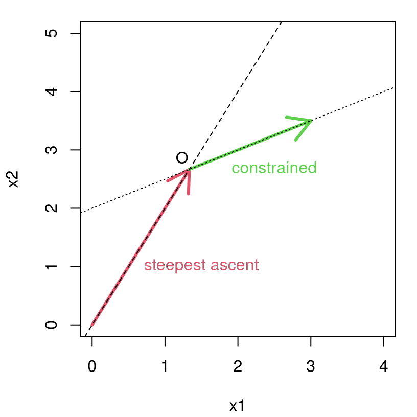

FIGURE 3.5: Modified path under constrained steepest ascent.

Although visually intuitive in two dimensions, the scheme requires a bit of math to operationalize more generally. That is, to determine the vector (in particular the direction) of ascent once the intersection point \(O\) is reached. Observe that the modified path can be parameterized by the vector \(b_j - d c_j\), for \(j=1,\dots,m\), for which

\[ \sum_{j=1}^m (b_j - d c_j)^2 \quad \mbox{is minimized.} \]

In other words, the direction along the constraint line (or plane) is taken so as to be the closest to the original path. Just like with our confidence region calculations above, this is another “funny regression” situation in which \(b_j\) are being regressed against \(c_j\), without an intercept, through which we calculate a coefficient \(d\), playing here the role of regression slope. Ordinary least squares calculations give

\[ d = \frac{\sum_{j=1}^m b_j c_j}{\sum_{j=1}^m c_j^2}. \]

Using that value, the modified portion of the path would begin at \(O\) and proceed in the direction described by an \(m\)-vector with components \(b_j - d c_j\), for \(j=1,\dots,m\). How to find the intersection point \(O\)? In our simple example we expressed the steepest ascent and constraint relationships as \(x_2\) in terms of \(x_1\). Setting the two \(x_2\) expressions equal to one another allowed us to solve for \(x_1\). That’s made more general as follows. We know that a steepest ascent path is given by \(x_j = \rho b_j\), for \(j=1,\dots,m\) and that \(c_0 + \sum_{j=1}^m c_j x_j = 0\) must also hold. Therefore, they collide at \(\rho_0\) satisfying

\[ c_0 + \left(\sum_{j=1}^m c_j b_j \right) \rho_o = 0. \quad\quad \mbox{Solving gives } \quad \rho_o = \frac{- c_0}{\sum_{j=1}^m c_j b_j}. \]

Using that calculation, coordinates of the intersection point are given as \(O = (x_1^o, \dots, x_m^o)\) where \(x_j^o = \rho_o b_j\), for \(j=1,\dots,m\). One may then move along the modified portion of the path, starting at \(O\), following

\[ x_j = x_j^o + \lambda(b_j - d c_j), \]

where \(d\) is determined by the least squares solution, above, and \(\lambda \geq 0\) is chosen by the practitioner. In this way the process for following the modified path is identical to that in Algorithm 3.1 except that the starting point is \(O\) rather than the zero-vector, and coefficient \(b_j\) is replaced by \(b_j - d c_j\).

Example: fabric strength

This example concerns the breaking strength in grams per square inch of a certain type of fabric as a function of three components \(\xi_1, \xi_2, \xi_3\). Raw data is unavailable, but Table 3.6 provides ranges from an experiment involving three input variables which are measured in grams.

TABLE 3.6: Summarizing fabric strength data.

Material	-1	+1
1	100	150
2	50	100
3	20	40

Consider a constraint on the first two variables, \(\xi_1\) and \(\xi_2\), as follows:

\[ \xi_1 + \xi_2 \leq 500. \]

The first step is to transform to coded variables, in particular mapping the constraint to coded variables. R code below derives constants involved in that enterprise.

upper <- c(150, 100, 40)
lower <- c(100, 50, 20)
scale <- (upper - lower)/2
shift <- scale + lower
toxi <- data.frame(scale=scale, shift=shift)
toxi

##   scale shift
## 1    25   125
## 2    25    75
## 3    10    30

That results in the following mapping,

\[ \begin{aligned} x_1 &= \frac{ \xi_1 - 125}{25} & x_2 &= \frac{\xi_2 - 75}{25} & x_3 &= \frac{\xi_3 - 30}{10}, \end{aligned} \] whose inverse is straightforward and will be provided below. Under this mapping the constraint reduces to

\[ 25 x_1 + 25 x_2 \leq 300, \]

which leads to the following constants \(c_0, c_1, c_2, c_3\):

c <- c(-300, 25, 25, 0)

Since we don’t have the data we can’t perform a fit, but suppose we have the following from an off-line analysis,

\[ \hat{y} = 150 + 1.7 x_1 + 0.8 x_2 + 0.5 x_3, \]

represented in R as b below.

b <- c(150, 1.7, 0.8, 0.5)

Now \(\rho_o\) can be calculated as …

rhoo <- -c[1]/sum(c[-1]*b[-1])
rhoo

## [1] 4.8

… and as a result the modified path starts at:

xo <- rhoo*b[-1]
xo

## [1] 8.16 3.84 2.40

Ordinary least squares provides \(d\).

d <- as.numeric(coef(lm(b[-1] ~ c[-1] - 1)))
d

## [1] 0.05

Then the coordinates of the hybrid path, including ordinary steepest ascent up to \(O\) and modified thereafter, are given by the following function of the quantities above. Step sizes are controlled with scale parameter (vector) \(\lambda\) specified by the practitioner.

hpath <- function(lambda, b, c, rhoo, d)
 {
  ## steepest ascent up to one step past the constraint boundary
  delta <- b/b[1]
  path <- matrix(0, ncol=length(b), nrow=1)
  while(1) {
    lpath <- nrow(path)
    path <- rbind(path, path[lpath,] + delta)
    if(c[1] + sum(path[lpath + 1,]*c[-1]) > 0) break
  }
    
  ## intersection point plus steps along the modified portion
  cpath <- rhoo*b
  for(i in 1:length(lambda)) {
    cpath <- rbind(cpath, rhoo*b + lambda[i]*(b - d*c[-1]))
  }
    
  ## pasting the hybrid path together and naming the rows and columns
  path <- rbind(path[1:lpath,], cpath)
  colnames(path) <- paste("x", 1:length(b), sep="")
  rownames(path) <- c(rep("u", lpath), "o", rep("c", length(lambda)))
  return(path)
 }

Notice that the function makes several assumptions, including

• lambda should not contain zero, but the zero setting (corresponding to intersection \(O\)) is automatically calculated and included in the hybrid path;
• the steepest ascent path must eventually violate the constraint, otherwise there’s an infinite loop;
• the baseline variable is \(x_1\), corresponding to \(j=1\) in Algorithm 3.1.

Evaluating hpath with a sequence of lambda values, chosen somewhat arbitrarily, provides coordinates along the hybrid steepest ascent and modified path.

lambda <- c(1,2,3,4)
path <- hpath(lambda, b[-1], c, rhoo, d)

Finally, we may use toxi to map the hybrid path to the natural scale before formatting it for display in Table 3.7.

A <- matrix(rep(toxi[,1], nrow(path)), ncol=ncol(path), byrow=TRUE)
B <- matrix(rep(toxi[,2], nrow(path)), ncol=ncol(path), byrow=TRUE)
pathxi <- A * path + B
colnames(pathxi) <- paste("xi", 1:3, sep="")
kable(pathxi, caption="Coordinates on hybrid path.")

TABLE 3.7: Coordinates on hybrid path.

	xi1	xi2	xi3
u	125.0	75.00	30.00
u	150.0	86.76	32.94
u	175.0	98.53	35.88
u	200.0	110.29	38.82
u	225.0	122.06	41.76
u	250.0	133.82	44.71
u	275.0	145.59	47.65
u	300.0	157.35	50.59
u	325.0	169.12	53.53
o	329.0	171.00	54.00
c	340.2	159.75	59.00
c	351.5	148.50	64.00
c	362.8	137.25	69.00
c	374.0	126.00	74.00

The first row is the center of the design region, and the tenth records point \(O\), both on the natural scale. Observe that most of the coordinates on the hybrid path are well outside of the bounding box of the original design. Perhaps it’s unwise to venture out into that region before performing a new experiment – potentially leading to a course correction – part way between the edge of that box and \(O\). With that logic, a good candidate for the center point of the new design may be the fourth or fifth step along the hybrid path:

pathxi[4:5,]

##   xi1   xi2   xi3
## u 200 110.3 38.82
## u 225 122.1 41.76

What to do if we encounter runs in a follow-up experiment that don’t show improvement in the response? This may indicate that the first-order model isn’t a good approximation. A notion of “locale” might not be appropriate in this wider design space. Higher-order modeling could help, motivating the methods in the next section.

3.2 Second-order response surfaces

We can only get so far with steepest ascent on first-order fits, even with interactions. Linear models only offer decent approximation locally. That local scope may in practice be exceedingly small, especially near the optimal input configuration. Eventually observed responses will systematically diverge from estimated ones along the steepest ascent path, at least for most interesting problems. Divergence could be substantial. When that happens it’s worth entertaining a richer class of models, the simplest of which is a second-order (linear) model.

As a reminder, the second-order model is characterized by the following linear equation.

\[ y = \beta_0 + \sum_{j=1}^m \beta_j x_j + \sum_{j=1}^m \beta_{jj} x_j^2 + \sum \sum_{j < k}^m \beta_{jk} x_j x_k + \varepsilon \]

I won’t spend much time on appropriate designs for second-order models. However it’s worth noting that, since the model contains \(1 + 2m +m(m-1)/2\) parameters, the design must therefore contain at least as many distinct locations in order for all unknown regression coefficients \(\beta\) to be estimable via least squares/likelihood-based methods. Moreover the design must contain at least three levels of each variable to estimate any pure quadratic terms. For more details on design for second-order models see Chapters 8–9 of Myers, Montgomery, and Anderson–Cook (2016).

3.2.1 Canonical analysis

All second-order response surface models have a stationary point which, as shown visually in Figures 1.5–1.8, may be a maximum, minimum, or a saddle point. When the stationary point is a saddle point, the model is sometimes called a saddle or minimax system. Detecting the nature of the system with a design focused around nearby operating conditions, and determining the location of the stationary point, represent an integral first step in second-order analysis. As in the direction of the path of steepest ascent, the nature and location of a stationary point depends on the signs and magnitudes of estimated coefficients. In particular, estimated interaction/pure quadratic effects play a vital role, and their standard errors convey uncertainty about local behavior of the system.

As a simple example to fix ideas before delving deeper, consider a fitted second-order model given by

\[\begin{equation} \hat{y} = 100 + 5 x_1 + 10 x_2 - 8 x_1^2 - 12 x_2^2 - 12 x_1 x_2. \tag{3.3} \end{equation}\]

Because \(m=2\), simple graphics can help determine the location and nature of the stationary point. The code chunk below defines the fit, and then evaluates it on a grid in a rectangular input domain.

second.order <- function(x1, x2)
 { 
  100 + 5*x1 + 10*x2 - 8*x1^2 - 12*x2^2 - 12*x1*x2
 }  

x1 <- x2 <- seq(-4, 4, length=100)
g <- expand.grid(x1, x2)
y <- matrix(second.order(g[,1], g[,2]), ncol=length(x2))

Figure 3.6 shows the fit in perspective (left) and image/contour (right) formats. Recall that lighter colors correspond to higher values.

par(mfrow=c(1,2))
persp(x1, x2, y, theta=30, phi=30, zlab="eta", expand=0.75, lwd=0.25)
image(x1, x2, y, col=cols)
contour(x1, x2, y, add=TRUE)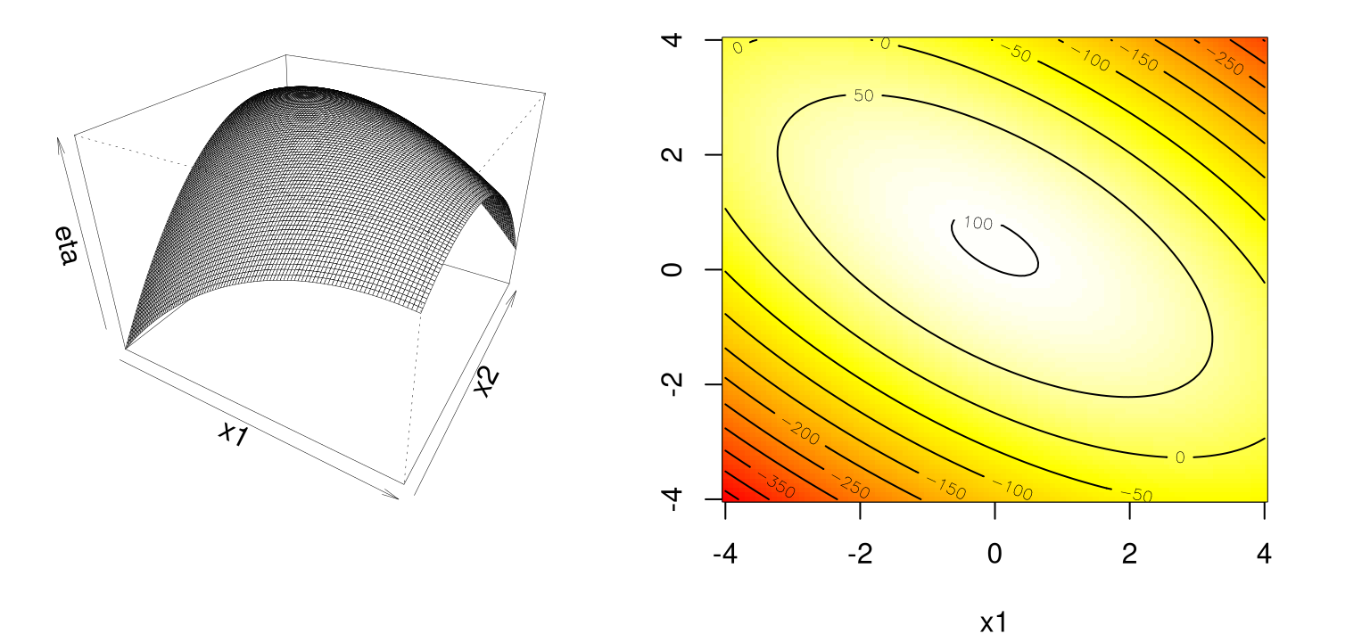

FIGURE 3.6: Simple maximum second-order response surface following Eq. (3.3).

By inspection, the response surface is concave down, a simple maximum like in Figure 1.5. Evidently it’s maximized near the origin, perhaps with \(x_2\) a little above zero. No need to ballpark it when we can find coordinates precisely. Calculus says that the stationary point is the solution to

\[ \frac{\partial \hat{y}}{\partial x_1} = 0 \quad \mbox{ and } \quad \frac{\partial \hat{y}}{\partial x_2} = 0. \]

This results in a system of linear equations …

\[ \begin{aligned} 16 x_1 + 12 x_2 &= 5 \\ 12 x_1 + 24 x_2 &= 10, \end{aligned} \]

… which can be solved in R as follows.

dy <- rbind(c(16, 12), c(12, 24))
xh <- solve(dy, c(5,10))
yh <- 100 + 5*xh[1] + 10*xh[2] - 8*xh[1]^2 - 12*xh[2]^2 - 12*xh[1]*xh[2]
c(x1=xh[1], x2=xh[2], y=yh)

##       x1       x2        y 
##   0.0000   0.4167 102.0833

Therefore, the stationary point is at \((\hat{x}_1, \hat{x}_2) = (0, 0.42)\), and the response value at that location is \(\hat{y}(\hat{x}) = 102.1\). To abstract a bit, towards obtaining a more generic recipe, it helps to write the fitted model in matrix notation as follows.

\[ \hat{y} = b_0 + x^\top b + x^\top B x \]

Above, the scalar \(b_0\), \(m\)-vector \(b\), and \(m \times m\) matrix \(B\) are estimates of intercept, linear (or main effects), and second-order coefficients, respectively. Specifically, \(B\) is the symmetric matrix

\[ B = \left[ \begin{array}{cccc} b_{11} & b_{12}/2 & \cdots & b_{1m}/2 \\ & b_{22} & \cdots & b_{2m}/2 \\ & & \ddots & \vdots \\ \mbox{sym.} & & & b_{mm} \end{array} \right] \]

containing all coefficients in front of features which are derived from original inputs (§3.2) through products \(x_j x_k\) giving

\[ x^\top B x = \sum_{j=1}^m b_{jj} x_j^2 + \sum \sum_{j < k}^m b_{jk} x_j x_k. \]

The \(1/2\) term arises due to the symmetry of \(B\), so that two contributions add up to one in the final sum. Setting up those quantities for our toy 2d example visualized in Figure 3.6 proceeds as follows in R.

b0 <- 100
b <- c(5, 10)
B <- matrix(c(-8, -12/2, -12/2, -12), ncol=2, byrow=TRUE)
B

##      [,1] [,2]
## [1,]   -8   -6
## [2,]   -6  -12

At first this representation (especially the \(B\) matrix) seems too clever by half. Are double-sums really that bad? But the investment is worth its weight in implementation simplicity, and in off-loading to matrix properties for interpretation. For example, in this formulation it’s straightforward to give a general expression for the location of the stationary point, \(x_s\). One can differentiate \(\hat{y}\) with respect to \(x\) to obtain

\[ \begin{aligned} \frac{\partial \hat{y}}{\partial x} &= b + 2 B x, \\ \mbox{giving} \quad x_s &= - \frac{1}{2} B^{-1} b \end{aligned} \]

after setting equal to zero and solving. The predicted response at the stationary point is obtained by plugging \(x_s\) back into the quadratic form for \(\hat{y}\):

\[ \begin{aligned} \hat{y}_s &= b_0 + x_s^\top b + x_s^\top B x_s\\ &= b_0 + x_s^\top b - \frac{1}{2} b^\top B^{-1} B x_s \\ &= b_0 + \frac{1}{2} x_s^\top b. \end{aligned} \]

Double-checking those formulas in R with our results above for the toy 2d example (3.3) indicates success.

xs <- - 0.5*solve(B) %*% b
ys <- b0 + 0.5*t(xs) %*% b
sols <- rbind(h=c(xh, yh), s=c(xs, ys))
colnames(sols) <- c("x1", "x2", "y")
sols

##   x1     x2     y
## h  0 0.4167 102.1
## s  0 0.4167 102.1

Now the nature of the stationary point is determined from the signs of the eigenvalues of the matrix \(B\), the relative magnitudes of which are key to interpretation. Such is the real value in investing in a matrix representation. Technically, location of the stationary point and its predicted response are not material to analysis of \(B\). However re-centering the system at \(x_s\) does aid interpretation. Translation and rotation of the axes, and inspection of eigenvalues described below, is referred to as the canonical analysis of the response system.

Toward that end, let \(z = x - x_s\) so that

\[ \begin{aligned} \hat{y} &= b_0 + (z + x_s)^\top b + (z + x_s)^\top B (z + x_s) \\ &= [b_0 + x_s^\top b + x_s^\top B x_s] + z^\top b + z^\top B z + 2 x_s^\top B z \\ &= \hat{y}_s + z^\top B z. \end{aligned} \]

Again, \(\hat{y}_s\) is the estimated response at the stationary point, and thus the final step comes from \(x_s = - \frac{1}{2} B^{-1} b\), giving \(2x_s^\top B z = -z^\top b\).

Once the system is centered at \(x_s\), the next step is to rotate axes according to their principal components – in other words, to determine the principal axes of contours of the response surface. Let \(P\) be an \(m \times m\) matrix whose columns contain normalized eigenvectors associated with eigenvalues of \(B\). Denote \(\Lambda = P^\top B P\) as the diagonal matrix of eigenvalues \(\lambda_1, \dots, \lambda_m\) corresponding to that system. Now, if \(w = P^\top z\), then

\[\begin{align} \hat{y} &= \hat{y}_s + w^\top P^\top B P w \notag \\ &= \hat{y}_s + w^\top \Lambda w \notag \\ &= \hat{y}_s + \sum_{j=1}^m \lambda_j w_j^2. \tag{3.4} \end{align}\]

These \(w_1, w_2, \dots, w_m\) are called canonical variables, and form the basis for principal axes. The final line in the equations above nicely describes the nature of the stationary point \(x_s\) via signs and relative magnitudes of eigenvalues \(\lambda_1, \dots, \lambda_m\).

1. If the \(\lambda_j\) are negative for all \(j\), the stationary point corresponds to a local maxima.
2. If \(\lambda_j\) are positive for all \(j\), we have a local minima.
3. If any \(\lambda_j\) and \(\lambda_k\) for \(j \ne k\) have mixed sign, we have a saddle point.

The development below explores some of these quantities on our running toy 2d example (Eq. (3.3) and Figure 3.6). To start with, eigenvalues may be calculated as follows.

E <- eigen(B)
lambda <- E$values
o <- order(abs(lambda), decreasing=TRUE)
lambda <- lambda[o]
lambda

## [1] -16.325  -3.675

Notice that both are negative, suggesting the stationary point \(x_s\) is a maximum. (We already knew that, but it doesn’t hurt to check understanding.) The code stores eigenvalues in decreasing order. Observe that the first principal axis is elongated relative to the other by nearly a factor of four. Actually those numbers are in units of squared distance in the input space, so the true scaling factor is more like two. Code below extracts eigenvectors, taking their ordering from the eigenvalues.

V <- E$vectors[,o]

These eigenvectors have unit norm, so it can help to scale them a bit when visualizing. Figure 3.7 shows principal axes estimated for this response surface, upscaling eigenvectors by a factor of ten so that they cover the entire range of \(x_1\) and \(x_2\).

image(x1, x2, y, col=cols)
contour(x1, x2, y, add=TRUE)
lines(c(-V[1,1], V[1,1])*10 + xs[1], c(-V[2,1], V[2,1])*10 + xs[2], lty=2)
lines(c(-V[1,2], V[1,2])*10 + xs[1], c(-V[2,2], V[2,2])*10 + xs[2], lty=2)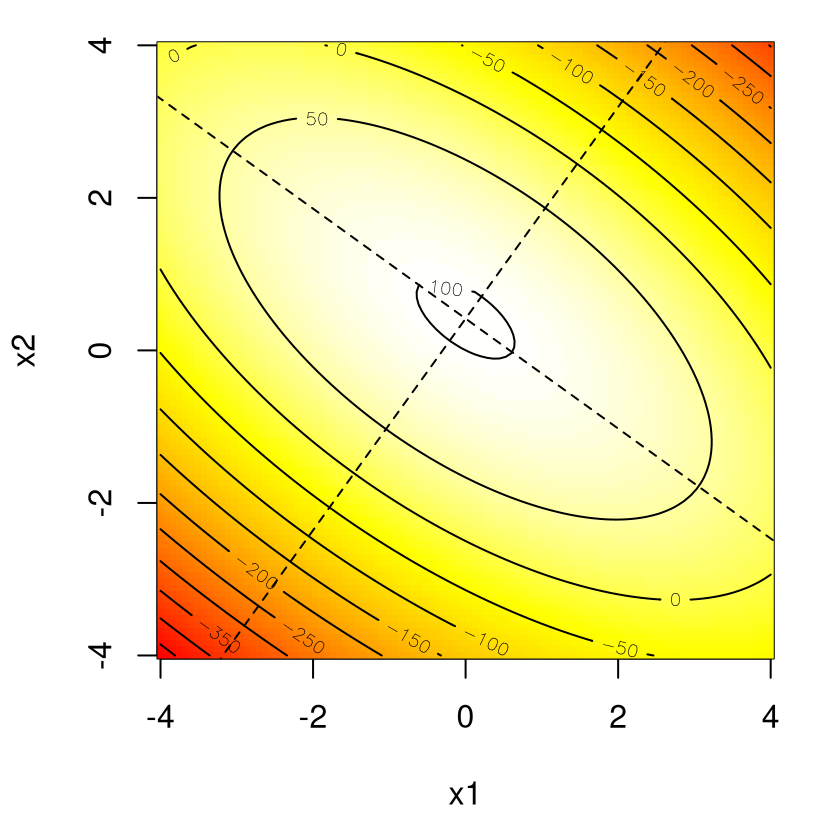

FIGURE 3.7: Principal axes for the response surface in Eq. (3.3).

When we work with the system in canonical variables through

\[ \hat{y} = 102.0833 -16.3246 w_1^2 -3.6754 w_2^2 \]

we’re essentially working on the original system pictured above, although there’s rarely a good reason to do so in practice. Eigenvalue analysis gives us all the information we need to proceed with further calculations, directly on original or coded inputs. Before outlining next steps, the example below provides a second look, but in a somewhat more realistic setting with a response surface estimated from actual data.

Example: chemical process

Consider an investigation into the effect of two variables, reaction temperature \((\xi_1)\) and reactant concentration \((\xi_2)\), on the percentage conversion of a chemical process \((y)\). By way of a bit of back-story, we arrived at the current setup after an initial screening experiment was conducted involving several factors, with temperature and concentration being isolated as the two most important variables. Since experimenters believed that the process was operating in the vicinity of the optimum, a quadratic model is appropriate for the next stage of analysis. Measurements of the response variables were subsequently collected on a central composite design whose center point was replicated four times.

chem <- read.table("chemical.txt", header=TRUE)
uchem <- unique(chem[,1:2])
reps <- apply(uchem, 1, 
  function(x) { sum(apply(chem[,1:2], 1, function(y) { all(y == x) })) })

Figure 3.8 provides a visualization of that design.

plot(uchem, type="n")
text(uchem, labels=reps)

FIGURE 3.8: Central composite design for an experiment involving a chemical process.

Note that the data file contains measurements in both natural and coded units. After expanding out into squared and interaction features, the second-order model may be fit to these data (in coded units) with the following code.

X <- data.frame(x1=chem$x1, x2=chem$x2, x11=chem$x1^2, x22=chem$x2^2, 
  x12=chem$x1*chem$x2)
y <- chem$y
fit <- lm(y ~ ., data=X)
kable(summary(fit)$coefficients, caption="Chemical process data.")

TABLE 3.8: Chemical process data.

	Estimate	Std. Error	t value	Pr(>|t|)
(Intercept)	79.750	1.2462	63.996	0.0000
x1	10.178	0.8812	11.551	0.0000
x2	4.216	0.8812	4.785	0.0030
x11	-8.500	0.9852	-8.628	0.0001
x22	-5.250	0.9852	-5.329	0.0018
x12	-7.750	1.2462	-6.219	0.0008

Observe in Table 3.8 that all estimated coefficients are statistically significant at the typical 5% level. The fitted model may be summarized as

\[ \hat{y} = 79.75 + 10.18 x_1 + 4.22 x_2 - 8.50 x_1^2 - 5.25 x_2^2 - 7.75 x_1 x_2. \]

To obtain some visuals, code below builds a predictive grid in natural inputs, and converts these into coded units for prediction.

r <- cbind(c(200, 250), c(15,25))
d <- (r[2,] - r[1,])/2
xi1 <- seq(min(chem$temp), max(chem$temp), length=100)
xi2 <- seq(min(chem$conc), max(chem$conc), length=100)
xi <- expand.grid(xi1, xi2)
x <- cbind((xi[,1] - r[2,1] + d[1])/d[1], (xi[,2] - r[2,2] + d[2])/d[2])

Using that grid in coded units, a data.frame of features is built, and fed into the predict.lm method.

XX <- data.frame(x1=x[,1], x2=x[,2], 
  x11=x[,1]^2, x22=x[,2]^2, x12=x[,1]*x[,2])
p <- predict(fit, newdata=XX)

Figure 3.9 shows an image/contour view into those predictions on natural axes.

xlab <- "Temperature (°C)"
ylab <- "Concentration (%)"
image(xi1, xi2, matrix(p, nrow=length(xi1)), 
  col=cols, xlab=xlab, ylab=ylab)
contour(xi1, xi2, matrix(p, nrow=length(xi1)), add=TRUE)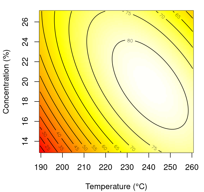

FIGURE 3.9: Fitted response surface for chemical process data whose fit is summarized in Table 3.8.

Canonical analysis begins by determining the location of stationary point \(x_s\). Essentially cutting-and-pasting from above …

b <- coef(fit)[2:3]
B <- matrix(NA, nrow=2, ncol=2)
diag(B) <- coef(fit)[4:5]
B[1,2] <- B[2,1] <- coef(fit)[6]/2
xs <- -(1/2)*solve(B, b)
xs

## [1]  0.62648 -0.06088

… which is converted back to natural units as follows.

xis <- xs*d + (r[2,] - d)
xis

## [1] 240.7  19.7

A check that this is correct is deferred until after we calculate canonical axes, below. Both eigenvalues of \(B\) are negative, so the stationary point is a maximum (as is obvious by inspecting the surface in Figure 3.9).

E <- eigen(B)
E

## eigen() decomposition
## $values
## [1]  -2.673 -11.077
## 
## $vectors
##         [,1]    [,2]
## [1,]  0.5537 -0.8327
## [2,] -0.8327 -0.5537

The code below saves those values, re-ordering them by magnitude, extracts eigenvectors (in that order), and converts them to their natural scale for visualization.

lambda <- E$values
o <- order(abs(lambda), decreasing=TRUE)
lambda <- lambda[o]
V <- E$vectors[,o]
Vxi <- V
for(j in 1:ncol(Vxi)) Vxi[,j] <- Vxi[,j]*d*10

We may then depict those axes, which intersect at stationary point \(x_s\), as in Figure 3.10.

image(xi1, xi2, matrix(p, nrow=length(xi1)), col=cols, xlab=xlab, ylab=ylab)
contour(xi1, xi2, matrix(p, nrow=length(xi1)), add=TRUE)
lines(c(-Vxi[1,1], Vxi[1,1])+xis[1], c(-Vxi[2,1], Vxi[2,1])+xis[2], lty=2)
lines(c(-Vxi[1,2], Vxi[1,2])+xis[1], c(-Vxi[2,2], Vxi[2,2])+xis[2], lty=2)
points(xis[1], xis[2])
text(xis[1], xis[2], "xs", pos=4)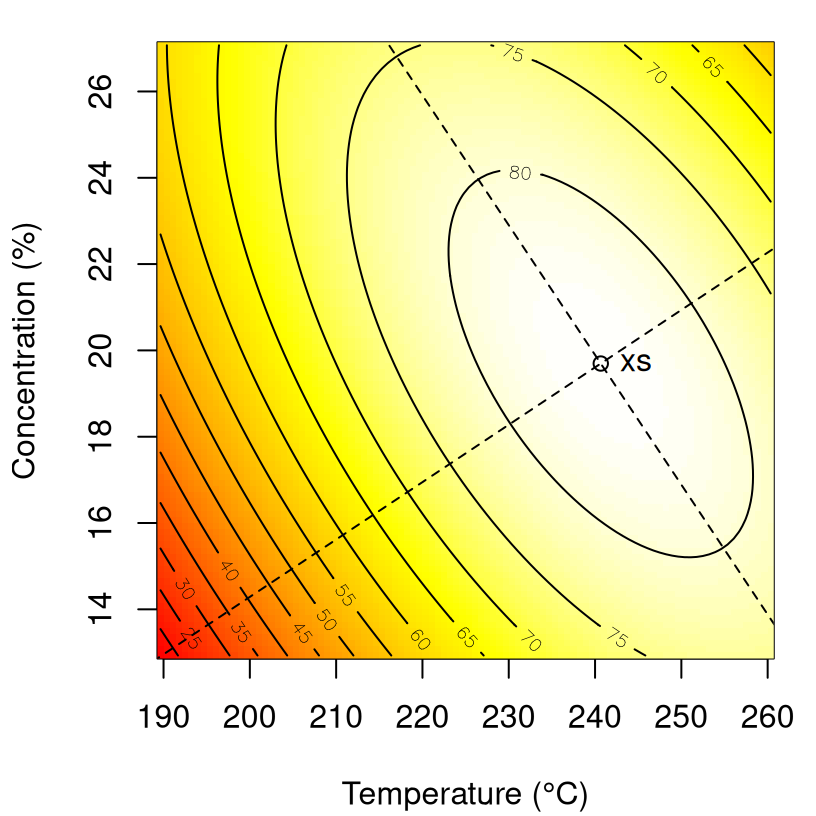

FIGURE 3.10: Principal axes for response surface in Figure 3.9.

The canonical form of the second-order model is

\[ \hat{y} = \hat{y}_s + \lambda_1 w_1^2 + \lambda_2 w_2^2, \]

where \(\hat{y}_s\) is computed as follows.

ys <- as.numeric(coef(fit)[1]) + drop(0.5*t(xs) %*% b)
ys

## [1] 82.81

So we have

\[ \hat{y} = 82.8099 -11.0769 w_1^2 -2.6731 w_2^2. \]

The input corresponding to \((w_1=0, w_2=0)\), which is \(x_s\) in coded units, is an obvious candidate for a confirmation test or as the center of a new central composite design over a narrower range of inputs. One potential criticism of this approach is that subsequent iterations retain little memory of previous (expensive) experimental work. Local second-order Taylor expansions are not well-suited to data collected at multiple – even somewhat nearby – locales. This will remain a motivating theme for much of the more global, nonparametric surrogate-based methods in later chapters. In the meantime, what happens when the eigenvalues aren’t all of the same sign?

3.2.2 Ridge analysis

When the system involves a pure minimum or maximum the procedure outlined above is fairly straightforward. But what happens when eigenvalues are mixed, or near zero? It’s perhaps more common for data on real response surfaces to lead to estimated models implying a degree of ambiguity. Saddle points are one possibility, although these are rather less common in practice, suggesting a bifurcation in the input space. A far more involved study may be required to choose between two or more competing locally optimal operating regimes on submanifolds of the study region. The murky spaces in-between, when some eigenvalues are approximately zero (and the others are of generally the same sign) are rather more common. This scenario indicates an elongation of the surface in the canonical direction corresponding to that eigenvalue, resulting in what’s called a ridge system. An expanded toolset is required, not only to deal with uncertainties regarding the nature of the system – to test for and detect the nature of ridges – but subsequently to decide how to iterate towards improved operating conditions: to “rise the ridge”.

Ridge systems are classified into two types depending on the estimated location of the stationary point \(x_s\), relative to the experimental design used to fit the second-order model. If \(x_s\) is within the region of the design then we have a stationary ridge system. This is a fortunate circumstance since it means that many inputs, along the ridge, provide nearly the same, almost optimal result. Practitioners therefore have some freedom to choose among operating conditions along that ridge, perhaps according to other criteria. For example if one setting along the ridge is easier to implement, or represents the smallest divergence from previous operating conditions, that setting might be preferred over others. On the other hand, if \(x_s\) isn’t inside the design region, this suggests that additional experimentation may be in order. We have a rising or falling ridge. Remote \(x_s\) may be spurious, so small steps in its direction are preferred over big jumps into a new regime. Any tests failing to reject a hypothesis about one or more zero eigenvalues, leading to a ridge local to the current design, will likely need to be re-evaluated in the new experimental region.

As a warm-up example to make things a little more concrete, consider data from an experiment on a square region with two factors, \(A\) and \(B\), using a central composite design with three center runs. Code supporting the second-order summary provided in Table 3.9 reads in data, expands into second-order features and performs the least squares fit.

rr <- read.table("risingridge.txt", header=TRUE)
rr$A2 <- rr$A^2
rr$B2 <- rr$B^2
rr$AB <- rr$A*rr$B
fit <- lm(y ~ ., data=rr)
kable(summary(fit)$coefficients, 
  caption="Linear model summary for rising ridge data.")

TABLE 3.9: Linear model summary for rising ridge data.

	Estimate	Std. Error	t value	Pr(>|t|)
(Intercept)	50.263	0.3894	129.079	0e+00
A	-12.417	0.3099	-40.068	0e+00
B	8.283	0.3099	26.730	0e+00
A2	-4.108	0.4769	-8.614	3e-04
B2	-9.108	0.4769	-19.098	0e+00
AB	11.125	0.3795	29.312	0e+00

Observe that \(t\)-tests indicate that all estimated coefficients are statistically significant. To perform the canonical analysis, let’s extract the coefficients into vector \(b\) and matrix \(B\), and use those values to estimate \(x_s\).

b <- coef(fit)[2:3]
B <- matrix(NA, nrow=2, ncol=2)
diag(B) <- coef(fit)[4:5]
B[1,2] <- B[2,1] <- coef(fit)[6]/2
xs <- -(1/2)*solve(B, b)
xs

## [1] -5.177 -2.707

Now, the bounding box of the design is …

apply(rr[,1:2], 2, range)

##       A  B
## [1,] -1 -1
## [2,]  1  1

… so \(x_s\) is well outside the experimental region. Eigen-analysis indicates that \(x_s\) is a maximum, as both estimated eigenvalues are negative. However one of them is quite close to zero.

E <- eigen(B)
lambda <- E$values
o <- order(abs(lambda), decreasing=TRUE)
V <- E$vectors[,o]*20
lambda <- lambda[o]
lambda

## [1] -12.7064  -0.5094

We’ll have to wait until §3.2.5 to say how close is close in statistically meaningful terms. Here the point is that statistically significant regression coefficients don’t necessarily imply that eigenvalues are (statistically) nonzero and vice versa. Coefficients can “cancel each other out” when they work in concert to represent the estimated response surface. The canonical form offers another view. Combining those eigenvectors and a calculation of \(\hat{y}_s\) …

ys <- coef(fit)[1] + 0.5*t(xs) %*% b
ys

##       [,1]
## [1,] 71.19

… leads to the representation

\[ \hat{y} = 71.1902 -12.7064 w_1^2 -0.5094 w_2^2. \]

So the question is: should we ignore the second canonical axis by taking \(\lambda_2^2 = 0\)? Although testing for \(\lambda_2^2 = 0\) is technically a matter of statistical inference, the outcome of that test is somewhat of a moot point since \(x_s\) is so far outside the design region, and the first principal axis has more than \(24 \times\) the “weight” of the second-one. For all practical purposes, we have a rising ridge scenario.

If that doesn’t make sense, perhaps the following visualization will help. Using the eigenvectors and gathering predictions on a grid of inputs (\(A\) and \(B\)) chosen large enough to show all relevant features, we obtain the picture provided by Figure 3.11.

x <- seq(-6, 6, length=100)
xx <- expand.grid(x, x)
XX <- data.frame(A=xx[,1], B=xx[,2], A2=xx[,1]^2, 
  B2=xx[,2]^2, AB=xx[,1]*xx[,2])
p <- predict(fit, newdata=XX)
image(x, x, matrix(p, nrow=length(x)), col=cols, xlab="A", ylab="B")
contour(x, x, matrix(p, nrow=length(x)), add=TRUE)
lines(c(-V[1,1], V[1,1]) + xs[1], c(-V[2,1], V[2,1]) + xs[2], lty=2)
lines(c(-V[1,2], V[1,2]) + xs[1], c(-V[2,2], V[2,2]) + xs[2], lty=2)
polygon(c(1,1,-1,-1), c(1,-1,-1,1), lty=3)
text(0,-0.5, "design region", cex=0.5)
points(xs[1], xs[2])
text(xs[1], xs[2], "xs", pos=4)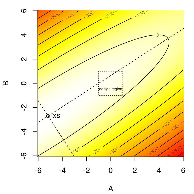

FIGURE 3.11: Visual of the rising ridge on principal axes whose stationary point \(x_s\) is far from the design region.

Regardless of whether or not \(\lambda_2^2\) is statistically zero, it’s both clear which way to move the experimental region (toward \(x_s\)) and foolish to trust \(x_s\) and move the experimental design all the way over there. It’s never a good idea to extrapolate too far outside the design region, especially with linear models. It’ll be beneficial to develop a more formal framework for deciding on next steps. When \(x_s\) is closer to or within the design region, and/or when \(\lambda\)s are similar in magnitude, a more nuanced analysis may be warranted. In such cases it’ll be crucial to link outcomes of statistical tests to knobs in our framework in order to cautiously but expediently rise the ridge.

Ridge analysis is steepest ascent applied to second-order models. Since second-order models are generally undertaken when the practitioner believes that s/he is quite near the region of the optimum, ridge analysis is typically entertained only in such settings. However, as we saw above, results from experiments may reveal a stationary point well outside the design region, contradicting that belief. Most often this is an artifact of the local nature of analysis via low-order polynomial (Taylor) approximation. Nevertheless, it’s important for practitioners to keep an open mind, and let evidence in the data be suggestive, if not entirely authoritative, nearby the experimental regime. But enough with disclaimers …

Consider the fitted second-order response surface model

\[ \hat{y} = b_0 + x^\top b + x^\top B x. \]

Without loss of generality, presume that the center of the design region is \(x_1 = \dots = x_m = 0\), likely in coded units. In steepest ascent with first-order models we optimized the fitted response surface under a constraint, lest the solution be out at infinity. While second-order response surfaces may not as acutely suffer from that pathology, it’s nevertheless a good idea to explore paths of steepest ascent with “baby steps”. In a ridge analysis, the custom is to maximize (or minimize) \(\hat{y}\) subject to the constraint

\[ x^\top x = R^2. \]

Lagrange multipliers facilitate optimization by differentiating

\[ L = b_0 + x^\top b + x^\top B x - \mu(x^\top x - R^2) \]

with respect to the vector \(x\).

\[ \frac{\partial L}{\partial x} = b + 2 B x - 2 \mu x \]

The constrained optimal stationary point is determined by setting that expression to zero and then solving for \(x\).

\[ \begin{aligned} (B - \mu I_m)x &= - \frac{1}{2} b \\ x &= - \frac{1}{2}(B - \mu I_m)^{-1} b \end{aligned} \]

Notice how that solution looks like a ridge regression estimator. Although a coincidence in terminology, that analogy serves as an easy way to remember the role of \(\mu\) in a ridge analysis.

Appropriate choices of \(\mu\) depend upon eigenvalues of \(B\), and whether ascent or descent is desired. If a) \(\mu > \lambda_{\max}\), the largest eigenvalue of \(B\), then \(x\) will be an absolute maximum for \(\hat{y}\) subject to the constraint; otherwise if b) \(\mu < \lambda_{\min}\), then the solution will be an absolute minimum. To get better intuition on why and how, consider the orthogonal matrix \(P\) that diagonalizes \(B\), i.e., \(P^\top B P = \Lambda\), where \(\Lambda = \mathrm{diag}(\lambda_1, \dots, \lambda_m)\). Now for \((B - \mu I)\), which must be inverted to find \(x\), we find that

\[ P^\top (B - \mu I) P = \Lambda - \mu I_m, \quad \mbox{ since } \quad P^\top P = I_m. \]

Observe that situation a) thus results in a negative definite \(B - \mu I_m\); and b) a positive definite one. This result suggests, but doesn’t guarantee that \(x\) corresponds to an absolute minima or maxima in \(\hat{y}\); see Draper (1963) for more details.

Before turning to an example, let’s codify the steps in the form of pseudocode for easy reference. Although applications of steepest ascent on ridge systems vary widely in practice, the essence is often a variation on themes outlined in Algorithm 3.2.

Algorithm 3.2: Steepest Ascent for Second-Order Models

Assume we wish to maximize a second-order response surface (ascent); let \(x_0\) be the design center, e.g., the origin in coded inputs.

Require fitted first-order model via intercept \(b_0\); \(m\)-vector of main effects \(b\); and matrix of second-order terms \(B\). The bounding box of the design region must also be on hand.

Then

1. Calculate eigenvalues of \(B\) and let \(\lambda_{\max}\) be the largest such value.
2. Choose \(\mu \geq \lambda_{\max}\), perhaps with equality to start out with.
3. Solve for \(x\), the constrained optimal stationary point

\[ x = - \frac{1}{2}(B - \mu I_m)^{-1} b. \]

4. Using that \(x\), calculate the implied radius \(R = \sqrt{x^\top x}\).
5. With \((\mu, R)\) pair calculated in Steps 3–4, initialize an iterative (perhaps interactive) exploration of \(x\) and \(\hat{y}(x) = b_0 + x^\top b + x^\top B x\) values and standard errors near the boundary of the design.
   • Increasing \(\mu\) will result in coordinates \(x\) nearer to \(x_0\), the design center.
   • Decreasing \(\mu\), maintaining \(\mu > \lambda_{\max}\), will push \(x\) outside of the design region.

Return the resulting collection of \((\mu, x, \hat{y})\) tuples and standard errors, possibly after first mapping back from coded to natural units.

Step 5 of Algorithm 3.2 might benefit from elaboration. One typical approach here is to perform a bisection-style or root-finding search for \((\mu, R)\) pairs which yield an \(x\) as close to the boundary of the design as possible. Often the initial \(\mu\)-value, \(\mu^{(1)} = \lambda_{\max}\), leads to an \(x\) which is well outside the design area, so a sensible search area may be in the range \((\mu^{(1)}, 10 \mu^{(1)})\), with larger orders of magnitude on the upper end possibly being required if an initial search fails to converge on a solution away from the boundary. Another variation, which is actually an embellishment on the previous theme, is to use root-finding to derive an adaptive grid of \(\mu\)-values based on a regular grid of \(R\)-values, with evenly spaced radius from \(R=0\) (implying \(\mu = \infty\)) to \(R=2\) in coded units. Both variations will be explored in some detail in our example below. Having a collection of \((\mu, x, \hat{y})\) tuples for a range of \(R\)s may be beneficial in determining where to center the next experimental design. In particular, an inspection of prediction intervals obtained for \(\hat{y}\) could help determine the point near, or just beyond the design boundary where quadratic growth in variance begins to dominate the nature of their spread.

Example: ridge analysis of a saddle

Consider a chemical process that converts 1,2-propanediol to 2,5-dimethylpiperazine, where a maximum conversion is sought as a function of the following coded factors:

\[\begin{align} x_1 &= \frac{\mbox{NH$_3$ level} - 102}{51} & x_2 &= \frac{\mbox{temp. } - 250}{200} \notag \\ x_3 &= \frac{\mbox{H$_2$O level} - 300}{200} & x_4 &= \frac{\mbox{H press. } - 850}{350} \tag{3.5}. \end{align}\]

The data file contains measurements of the response on inputs (in those coded units) following a central composite design. R code below reads in the data and expands the resulting data.frame to include features of a second-order model. A short-hand is used to avoid the tedium of writing out all terms by hand. Some of the renaming and reordering of columns isn’t strictly necessary, but helps here to maintain a degree of consistency across analyses.

saddle <- read.table("saddle.txt", header=TRUE)
saddle <- cbind(saddle[,-5]^2, 
  model.matrix(~ .^2 - 1, saddle[,-5]), y=saddle[,5])
names(saddle)[1:4] <- paste("x", 1:4, 1:4, sep="")
names(saddle)[9:14] <- sub(":x", "", names(saddle)[9:14])
saddle <- saddle[c(5:8,1:4,9:15)]

A summary of the fit, provided in Table 3.10, suggests that perhaps we don’t have enough data (\(n = 25\)) for all of the estimated quantities (\(m=14\)). By independent \(t\)-tests at the 5% level – a crude inspection to be sure – there are far fewer useful than useless predictors.

fit <- lm(y ~ ., data=saddle)
kable(summary(fit)$coefficients, 
  caption="Summary of second-order fit to saddle data (3.5).")

TABLE 3.10: Summary of second-order fit to saddle data (3.5).

	Estimate	Std. Error	t value	Pr(>|t|)
(Intercept)	40.1982	8.322	4.8305	0.0007
x1	-1.5110	3.152	-0.4794	0.6420
x2	1.2841	3.152	0.4074	0.6923
x3	-8.7390	3.152	-2.7725	0.0197
x4	4.9548	3.152	1.5720	0.1470
x11	-6.3324	5.035	-1.2575	0.2371
x22	-4.2916	5.035	-0.8523	0.4140
x33	0.0196	5.035	0.0039	0.9970
x44	-2.5059	5.035	-0.4976	0.6295
x12	2.1938	3.517	0.6238	0.5467
x13	-0.1437	3.517	-0.0409	0.9682
x14	1.5813	3.517	0.4496	0.6626
x23	8.0063	3.517	2.2765	0.0461
x24	2.8062	3.517	0.7979	0.4435
x34	0.2937	3.517	0.0835	0.9351

Recall that a representation on canonical axes hinges on fewer (\(m+1 = 5\)) derived quantities. So nevertheless we proceed, prudently with caution. First, extract coefficient main effects vector \(b\) and matrix \(B\) of second-order terms.

b <- coef(fit)[2:5]
B <- matrix(NA, nrow=4, ncol=4)
diag(B) <- coef(fit)[6:9]
i <- 10
for(j in 1:3) {
  for(k in (j+1):4) {
    B[j,k] <- B[k,j] <- coef(fit)[i]/2
    i <- i + 1
  }
}

Using those coefficients, stationary point \(x_s\) may be calculated as follows.

xs <- -(1/2)*solve(B, b)
xs

## [1] 0.2647 1.0336 0.2906 1.6680

Observe that this is within the vicinity of the design region.

apply(saddle[,1:4], 2, range)

##        x1   x2   x3   x4
## [1,] -1.4 -1.4 -1.4 -1.4
## [2,]  1.4  1.4  1.4  1.4

Visualization is somewhat more challenging in four input dimensions, making eigen-analysis crucial from both interpretive and algorithmic perspectives.

E <- eigen(B)
lambda <- E$values
o <- order(abs(lambda), decreasing=TRUE)
lambda <- lambda[o]
lambda

## [1] -7.547 -6.008  2.604 -2.159

Evidently we have a saddle point: these coefficients are far from zero but don’t agree on sign. Of course, we don’t have their standard errors so we don’t know if they’re statistically non-zero. (Chances are not good, since so many of the estimated coordinates of \(b\) and \(B\) are likely insignificant. More later.) Stationary point \(x_s\), being centered on the trough of the saddle, is well-within the design region, so we’re in a somewhat different situation compared to our warm-up example from Table 3.9, where the center of the design was clearly along a ridge far from the estimated mode.

On the other hand, when choosing initial \(\mu^{(1)} = \lambda_{\max}\) and calculating the \(x\) this implies, following Steps 2–3 in Algorithm 3.2 …

mul <- max(lambda)
x <- solve(B - mul*diag(4), -b/2)
x

## [1] 1.163e+13 8.290e+13 1.297e+14 2.829e+13

… we get a location which is well outside of the design region. So a bit of work will be required to iterate on larger \(\mu\)-values, placing us closer to the boundary of the design region. To automate that process, code below sets up function f to serve as an objective in the search for that boundary via the root (i.e., zero-crossing) of \(R^2 - x^\top x\), with \(x\) derived as a function of \(\mu\). By default, f is set up to target \(R^2 = 1\) unless otherwise specified.

f <- function(mu, R2=1) 
 {
  x <- solve(B - mu*diag(4), -b/2)
  R2 - t(x) %*% x
 }

The boundary of our search region is at \(1.4\) in absolute value. We know that we need a \(\mu > \lambda_{\max}\), so it’s reasonable to set \(\mu = \lambda_{\max}\), stored as mul in the code, as the left-hand side of the search interval. For starters, we’ll search up to \(10 \lambda\) on the right.

mu <- uniroot(f, c(mul, 10*mul), R2=1.4^2)$root
mu

## [1] 4.834

Having located a \(\mu\)-value in the interior of the search region \([\lambda_{\max}, 10\lambda_{\max}]\), we can be confident that there’s no need to widen the range. It makes sense to check that input x associated with that \(\mu\)-value lies near one of the boundaries.

x <- solve(B - mu*diag(4), -b/2)
x

## [1] -0.09124 -0.47679 -1.29616  0.21061

Indeed, the third coordinate is quite close to \(1.4\). Double-checking the \(R\)-value …

drop(sqrt(t(x) %*% x))

## [1] 1.4

… verifies that the desired solution has been found. Since our \(x\) is within the design region, i.e., where predictions from the fitted second-order model are most reliable, this may represent a decent location for a confirmation test. Or it may serve as the center of a new design in an iteration along a path of ascent. But before doing that, it’s a good idea to inspect predictive standard errors, and corresponding error-bars. To avoid benchmarking in a vacuum, code below considers a range of \(R\)-values in \([0,2]\), and the \(\mu\)’s and \(x\)’s they imply, so that ultimately predictive equations can be derived at those locations, and compared relative to one another.

mus <- rs <- seq(0.1, 2, length=20)
xp <- matrix(NA, nrow=length(rs), ncol=4)
colnames(xp) <- c("x1", "x2", "x3", "x4")
for(i in 1:length(rs)) {
  mus[i] <- uniroot(f, c(mul, 100*mul), R2=rs[i]^2)$root
  xp[i,] <- solve(B - mus[i]*diag(4), -b/2)
}
xp <- rbind(rep(0,4), xp)
rs <- c(0, rs)
mus <- c(Inf, mus)

Obtaining predictions with those \(x\)-values requires expanding out into second-order features. Code below builds up a data.frame that can be passed into the predict.lm method.

Xp <- data.frame(xp)
Xp <- cbind(Xp^2, model.matrix(~ .^2 - 1, Xp))
names(Xp)[1:4] <- paste("x", 1:4, 1:4, sep="")
names(Xp)[9:14] <- sub(":x", "", names(Xp)[9:14])
Xp <- Xp[c(5:8,1:4,9:14)]

We’re ready to predict.

p <- predict(fit, newdata=Xp, se.fit=TRUE)

An inspection of the sequence(s) of numbers thus calculated, as collated in Table 3.11, reveals that predictive uncertainly grows very quickly away from the design boundary. It certainly seems risky to trust predictions derived from \(R > 1.4\).

kable(cbind(R=rs, mu=mus, data.frame(pred=p$fit, se=p$se.fit), round(xp,6)),
  caption="Predictions for the saddle experiment calculated along a path
  leading away from the center of the design region.")

TABLE 3.11: Predictions for the saddle experiment calculated along a path leading away from the center of the design region.

R	mu	pred	se	x1	x2	x3	x4
0.0	Inf	40.20	8.322	0.0000	0.0000	0.0000	0.0000
0.1	49.811	41.21	8.305	-0.0126	0.0064	-0.0871	0.0471
0.2	24.557	42.20	8.255	-0.0217	0.0012	-0.1773	0.0900
0.3	16.343	43.18	8.175	-0.0287	-0.0141	-0.2699	0.1271
0.4	12.368	44.16	8.074	-0.0346	-0.0379	-0.3641	0.1575
0.5	10.071	45.16	7.960	-0.0399	-0.0686	-0.4591	0.1815
0.6	8.598	46.18	7.849	-0.0451	-0.1045	-0.5543	0.1994
0.7	7.585	47.22	7.757	-0.0503	-0.1444	-0.6494	0.2120
0.8	6.853	48.30	7.708	-0.0556	-0.1873	-0.7438	0.2203
0.9	6.302	49.42	7.724	-0.0612	-0.2325	-0.8377	0.2248
1.0	5.875	50.57	7.832	-0.0669	-0.2793	-0.9308	0.2262
1.1	5.534	51.77	8.056	-0.0727	-0.3275	-1.0231	0.2251
1.2	5.257	53.01	8.414	-0.0788	-0.3765	-1.1148	0.2220
1.3	5.027	54.29	8.921	-0.0849	-0.4264	-1.2058	0.2170
1.4	4.834	55.62	9.581	-0.0912	-0.4768	-1.2961	0.2106
1.5	4.670	57.00	10.395	-0.0976	-0.5276	-1.3860	0.2030
1.6	4.528	58.42	11.357	-0.1041	-0.5789	-1.4752	0.1942
1.7	4.404	59.90	12.461	-0.1107	-0.6304	-1.5641	0.1846
1.8	4.296	61.42	13.699	-0.1173	-0.6821	-1.6525	0.1742
1.9	4.199	62.99	15.062	-0.1241	-0.7340	-1.7405	0.1631
2.0	4.114	64.61	16.543	-0.1308	-0.7861	-1.8281	0.1514

Perhaps the case is better made visually. Figure 3.12 plots confidence intervals (CIs) derived from these means and standard errors.

plot(rs, p$fit, type="b", ylim=c(20,100), xlab="radius (R)", 
   ylab="y.hat(x) & 95% CIs")
lines(rs, p$fit + 2*p$se, col=2, lty=2)
lines(rs, p$fit - 2*p$se, col=2, lty=2)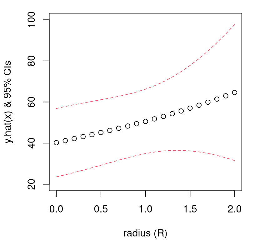

FIGURE 3.12: Visualizing predictive means and quantiles from Table 3.11.

Not surprisingly, predictive CIs begin to rapidly diverge from one another as we leave the design region, with \(R > 1.4\). Observe that the amount of predicted improvement (from the predictive mean), even at \(R=2\) (compared to \(R=0\)), is apparently dwarfed by estimation uncertainty. This suggests we need more runs inside/nearby the design region before venturing farther afield. It may be sensible to augment with a design centered near the \(R=1.4\) solution, collecting new responses in a more limited range of inputs. Combining these with the original design should yield improved predictions and further inform on statistical relevance for coefficients and eigenvectors/values underpinning the analysis. Assessing that relevance will require a bit more scaffolding, making for a nice segue into our final classical response surfaces segment(s), on sampling properties.

3.2.3 Sampling properties

The stationary point \(x_s\), or its constrained analog, are only estimates. Any point on the contour of a response surface, as well as the contour itself, possesses sampling variability. These quantities depend on estimated coefficients \(b_0\), \(b\) and \(B\), which have standard errors. When uncertainties are propagated through predictive equations to build the fitted response surface, and its constrained optima, those derived quantities inherit a sampling uncertainty which is, as yet, unexplored in our development. Below we review that predictive distribution, borrowing highlights from a first course in linear models, as a first step in understanding how uncertainty propagates to the stationary point(s) of the fitted surface, and steps along the path of steepest ascent.

Let \(y = (y_1,\dots, y_n)\) be an \(n\)-vector of responses and write \(X\) as the \(n \times (1+2m+{m \choose 2})\) model matrix comprised of rows \(x_i\) built, e.g., as

\[ \begin{aligned} x_i^\top &= [1, x_{i1}, x_{i2}, x_{i1}^2, x_{i2}^2, x_{i1}x_{i2}], && \mbox{for the special case of $m=2$.}\\ \mbox{Then we have } \quad b &= (X^\top X)^{-1} X^\top y, && \mbox{generally for any $X$.} \end{aligned} \]

For the time being, note that we’re not utilizing the \((b_0, b, B)\) representation, but rather a flattened \(p\)-vector of regression coefficients \(b\), arising from a feature expanded \(X\) encoding second-order model structure. Solution \(b = (X^\top X)^{-1} X^\top y\) comes from solving least squares equations, or as maximum likelihood estimator (MLE) \(b \equiv \hat{\beta}\) under the model \(Y \sim \mathcal{N}_n(X \beta, \sigma^2 \mathbb{I}_n)\), where \(\mathcal{N}_n\) is an \(n\)-variate multivariate normal (MVN) distribution.

Now a useful property of projections of MVN random vectors is that if \(Y \sim \mathcal{N}_n(\mu, \Sigma)\) and \(P\) is a \(p\times n\) matrix, then \(PY \sim \mathcal{N}_p(P \mu, P \Sigma P^\top\)). Notice that \(b\) involves one such projection. In particular, let \(P = (X^\top X)^{-1} X^\top\) so that \(\hat{\beta} = Py\). Observe that

• \(P X \beta = (X^\top X)^{-1} X^\top X \beta = \beta\), and
• \(P P^\top = (X^\top X)^{-1} X^\top X (X^\top X)^{-1} = (X^\top X)^{-1}\)

since \(X^\top X\) and its inverse are symmetric. Using the MVN result above, we obtain

\[\begin{equation} \hat{\beta} = PY \sim \mathcal{N}_p (\beta, \sigma^2 (X^\top X)^{-1}), \tag{3.6} \end{equation}\]

giving the sampling distribution of \(b \equiv \hat{\beta}\).

Predictions, provided as \(\hat{y}(x) \equiv x^\top b\), are a function of estimated \(b\) and thus inherit its sampling distribution. That distribution may be derived through a second projection, this time onto the (one-dimensional) real line. We obtain that \(\hat{y}(x)\) is univariate Gaussian with mean \(x^\top \beta\), which is the true (but unknown) response modulo the local nature of the approximation of the second-order response surface, with variance equal to \(\sigma^2 x^\top (X^\top X)^{-1} x\).

Usually \(\sigma^2\) is unknown, so it too must be estimated from data. MLE \(\hat{\sigma}^2\) may be derived as a mean sum of squares

\[ \begin{aligned} \hat{\sigma}^2 &= \frac{1}{n} \sum_{i=1}^n (y_i - x_i^\top b)^2, && \mbox{however} & s^2 &= \frac{1}{n-p}\sum_{i=1}^n (y_i - \hat{y}_i)^2, \end{aligned} \]

which corrects for bias in \(\hat{\sigma}^2\) by subtracting off \(p\) DoF spent in estimating \(b\), is more often used in practice. An application of Cochran’s Theorem gives that \(s^2 \sim \frac{\sigma^2}{n-p}\chi_{n-p}^2\). The Gaussian nature of \(Y(x) \mid \sigma^2\) and \(\chi^2\) relationship between \(s^2\) and \(\sigma^2\) combines to give a Student-\(t\) sampling distribution for the prediction

\[ \begin{aligned} \hat{y}(x) &\sim t_{n-p}(x^\top \beta, s_{\hat{y}}^2(x)), & \mbox{ as shorthand for } && \frac{\hat{y}(x) - x^\top \beta}{s_{\hat{y}}(x)} &\sim t_{n-p}, \end{aligned} \]

where \(s_{\hat{y}}(x)\) is the standard error of \(\hat{y}(x) \equiv x^\top b\):

\[ s_{\hat{y}(x)} = s \sqrt{x^\top (X^\top X)^{-1} x}. \]

When using predict.lm with fitted lm objects in R, argument se.fit=TRUE causes estimates of \(s_{\hat{y}(x)}\) to be returned on output. Given that standard error, a CI for \(\hat{y}(x)\) is \(\hat{y}(x) \pm t_{\alpha/2,n-p} s_{\hat{y}(x)}\). In R this is what you get when you provide interval="confidence" to predict with level=1 - alpha. Note that this is different from a prediction interval whose standard error includes an extra factor of \(s\):

\[ \sqrt{s^2 + s_{\hat{y}(x)}^2}. \]

You get intervals based on this estimate with interval="prediction". For completeness, let me remark that a similar argument, paired with the Gaussian sampling distribution (3.6) leads to the quantities reported for \(b_j \equiv \hat{\beta}_j\) in summary.lm output, e.g. most recently in Table 3.9. The square-root of the diagonal of \(s (X^\top X)^{-1}\) are the standard errors \(s_{b_j}\) from Eq. (3.2), also on \(n-p\) DoF.

To illustrate a predictive application, consider again our chemical conversion “saddle” example (3.5) on four input variables. Since visualization is challenging in 4d, here we explore how predictive standard error varies as a function of \((x_1, x_2)\) under fixed settings of \((x_3^0,x_4^0)\) values. First, set up a 2d grid in the first two inputs to aid in visualization via slices.

x12 <- seq(-2,2,length=100)
g <- expand.grid(x12, x12)
Xp <- data.frame(x1=g[,1], x2=g[,2], 
  x11=g[,1]^2, x22=g[,2]^2, x12=g[,1]*g[,2])

Code below completes the data.frame with features derived from two settings of the latter two inputs, \((x_3,x_4)=(0,0)\) and \((x_3,x_4) = (1,1)\), and collects predictive quantities under the response surface fit earlier.

## x3 = x4 = 0
Xp$x3 <- Xp$x33 <- Xp$x4 <- Xp$x44 <- Xp$x34 <- 0
Xp$x13 <- Xp$x14 <- Xp$x23 <- Xp$x24 <- Xp$x34 <- 0
p0 <- predict(fit, newdata=Xp, se.fit=TRUE)
## x3 = x4 = 1
Xp$x3 <- Xp$x33 <- Xp$x4 <- Xp$x44 <- Xp$x34 <- 1
Xp$x13 <- Xp$x14 <- Xp$x1; Xp$x23 <- Xp$x24 <- Xp$x2
p1 <- predict(fit, newdata=Xp, se.fit=TRUE)

Surfaces showing the predictive standard error \(s_{\hat{y}(x)}\) in those two cases are provided in Figure 3.13. Projected experimental design coordinates are overlayed as open circles; the subset of inputs lying in the corresponding \((x_3, x_4)\) slice are shown as closed circles.

par(mfrow=c(1,2))
bs <- seq(min(p0$se.fit), max(p0$se.fit), length=129)
image(x12, x12, matrix(p0$se.fit, nrow=length(x12)), col=cols, breaks=bs,
    xlab="x1", ylab="x2", main="se.fit, x3 = x4 = 0")
contour(x12, x12, matrix(p0$se.fit, nrow=length(x12)), add=TRUE)
points(saddle[,1:2])
points(saddle[apply(saddle[,3:4] == c(0,0), 1, all),1:2], pch=19)
image(x12, x12, matrix(p1$se.fit, nrow=length(x12)), col=cols, breaks=bs,
    xlab="x1", ylab="x2", main="se.fit, x3 = x4 = 1")
contour(x12, x12, matrix(p1$se.fit, nrow=length(x12)), add=TRUE)
points(saddle[,1:2])
points(saddle[apply(saddle[,3:4] == c(1,1), 1, all), 1:2], pch=19)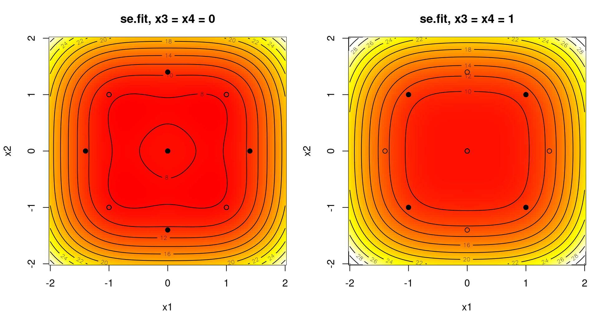

FIGURE 3.13: Predictive variance slices for the chemical conversion “saddle” example (3.5).

What do we take away from these plots? Prediction with this second-order response surface becomes worse as one gets near the design perimeter. If the predicted value of the optimum isn’t inside the design region, searching outside comes with substantial risk. Observe that \((X^\top X)^{-1}\) plays a prominent role in \(s_{\hat{y}(x)}\), so the design \(X\) matters! What might be less obvious is that \(X\) (and \(y\)) also affect the location of the (estimated) stationary point \(x_s\) and its nature. So if we’re wondering about uncertainty in \(\hat{y}(x_s)\), say, we’re missing an important source of variability.

3.2.4 Confidence in the stationary point

Clearly the location of the stationary point \(x_s\) is of considerable interest in its own right, beyond its out-sized role in a ridge analysis. But how good can an estimate based on local second-order modeling and limited experimentation possibly be? Can we get a sense of confidence in our estimates? Could uncertainty so swamp our estimates that another set of locations offers about the same improvement at far lower risk? Answering these questions requires propagating predictive standard error through the derivative-based optimization.

Recall that

\[ \begin{aligned} \hat{y}(x) &= b_0 + x^\top b + 2 x^\top B x, && \mbox{where we calculated} & \frac{\partial \hat{y}(x)}{\partial x} &= b + 2 B x. \end{aligned} \]

So let \(d(x) = b + 2 B x\) be the vector of derivatives (the gradient) with each component being \(d_j(x) = b_j + 2 B_j x\), where \(B_j\) is the \(j^{\mathrm{th}}\) row of \(B\). Observe that \(d(x)\) is comprised of linear functions of \(x_1, \dots, x_m\). Now let \(t=(t_1,t_2, \dots, t_m)\) denote the true but unknown stationary point of the system. The Gaussian error structure of our linear modeling framework, and the fact that \(t\) is a critical point of the true response surface, implies that

\[ d(t) \sim \mathcal{N}_m(0, \mathbb{V}\mathrm{ar}\{d(t)\}). \]

This is useful because, if we can obtain an estimate of that variance–covariance matrix, we may use the following result as a means of developing a CI for \(t\), the true location of the stationary point:

\[\begin{equation} \frac{d^\top(t) [\widehat{\mathbb{V}\mathrm{ar}}\!\{d(t)\}]^{-1} d(t)}{m} \sim F_{m, n-p}, \tag{3.7} \end{equation}\]

where \(\widehat{\mathbb{V}\mathrm{ar}}\!\{d(t)\}\) is \(\mathbb{V}\mathrm{ar}\{d(t)\}\) with \(\sigma^2\) estimated by \(s^2\) on \(n-p\) DoF. In particular, a \(100(1-\alpha)\)% confidence region for the stationary point includes those \(t\) which evaluate, under that quadratic form (3.7), to a number less than an \(\alpha\) quantile of the \(F_{m, n-p}\) distribution:

\[\begin{equation} d^\top(t) [\widehat{\mathbb{V}\mathrm{ar}}\!\{d(t)\}]^{-1} d(t) \leq m F^\alpha_{m, n-p}. \tag{3.8} \end{equation}\]

The utility of this result is, however, unfortunately limited to graphical analysis in two or three dimensions at most. Also, the devil is in the details of estimating the variance of the derivatives, which is greatly simplified if the design is chosen fortuitously. That’s best illustrated by example.

Consider data on a process in two coded input dimensions under a central composite design whose center is replicated four times.

crdat <- read.table("confreg.txt", header=TRUE)

R code below combines several steps: expanding to second-order features, model fitting and extracting \(b\) and \(B\), differentiating and solving to estimate stationary point \(x_s\).

crdat$x11 <- crdat$x1^2
crdat$x22 <- crdat$x2^2
crdat$x12 <- crdat$x1 * crdat$x2
fit <- lm(y ~ ., data=crdat)
b <- coef(fit)[2:3]
B <- matrix(NA, nrow=2, ncol=2)
diag(B) <- coef(fit)[4:5]
B[1,2] <- B[2,1] <- coef(fit)[6]/2
xs <- -(1/2)*solve(B, b)
xs

## [1] -0.1716 -0.1806

Stationary point \(x_s\) is a maximum, as indicated by the eigenvalues.

eigen(B)$values

## [1] -2.244 -3.061

Next evaluate predictive equations on a grid in order to visualize the response surface, design and stationary point, which is well within the interior of the experimental region. See Figure 3.14.

xx <- xx <- seq(-1.6, 1.6, length=200)
g <- expand.grid(xx, xx)
XX <- data.frame(x1=g[,1], x2=g[,2], 
  x11=g[,1]^2, x22=g[,2]^2, x12=g[,1]*g[,2])
p <- as.numeric(predict(fit, newdata=XX))
image(xx, xx, matrix(p, nrow=length(xx)), col=cols, xlab="x1", ylab="x2")
contour(xx, xx, matrix(p, nrow=length(xx)), add=TRUE)
points(crdat$x1, crdat$x2, pch=20)
points(xs[1], xs[2])
text(xs[1], xs[2], "xs", pos=4)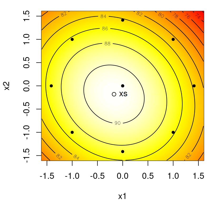

FIGURE 3.14: Simple maximum response surface.

Combining \(d(t) = b + 2 B t\) with calculations of b and B …

d <- rbind(c(b[1], 2*B[,1]), c(b[2], 2*B[,2]))
colnames(d) <- c("(Intercept)", "t1", "t2")
d

##      (Intercept)     t1     t2
## [1,]      -1.095 -5.562 -0.775
## [2,]      -1.045 -0.775 -5.047

… gives the following expressions for derivatives of the response surface as a function of the true unknown stationary point \(t\).

\[ \begin{aligned} d_1(t) &= -1.095 - 5.562 t_1 - 0.775 t_2 \\ d_2(t) &= -1.045 - 0.775 t_1 - 5.048 t_2 \end{aligned} \]

Now the variances of \(d(t)\), via \(\hat{\beta} \sim \mathcal{N}_p(\beta, \sigma^2 (X^\top X)^{-1}\)), are obtained from our estimate of the residual variance \(s^2\) and the matrix \((X^\top X)^{-1}\). The former may be extracted from fit …

s2 <- summary(fit)$sigma^2
s2

## [1] 3.164

… on \(n-p=7\) DoF. The latter is most easily calculated “by hand” as follows.

X <- cbind(1, as.matrix(crdat[,-3]))
XtXi <- solve(t(X) %*% X)
XtXi

##                x1    x2      x11      x22  x12
##      0.3333 0.000 0.000 -0.16669 -0.16669 0.00
## x1   0.0000 0.125 0.000  0.00000  0.00000 0.00
## x2   0.0000 0.000 0.125  0.00000  0.00000 0.00
## x11 -0.1667 0.000 0.000  0.17716  0.05208 0.00
## x22 -0.1667 0.000 0.000  0.05208  0.17716 0.00
## x12  0.0000 0.000 0.000  0.00000  0.00000 0.25

Observe that \((X^\top X)^{-1}\) is sparse, owing to the orthogonal structure of our central composite design. We finally have all necessary ingredients to build up the covariance matrix of \(d(t)\), as a function of \(t\). We shall proceed one component at a time. First: diagonal elements. By linearity of variances, and reading off entries of \((X^\top X)^{-1}\), we obtain

\[ \begin{aligned} \widehat{\mathbb{V}\mathrm{ar}}\{ d_1(t) \} &= \frac{s^2}{\sigma^2}[ \mathbb{V}\mathrm{ar} b_1 + 4 t_1^2 \mathbb{V}\mathrm{ar} b_{11} + t_2^2 \mathbb{V}\mathrm{ar} b_{12} ] \\ &= s^2 [1/8 + 4 t_1^2 (0.1772) + t_2^2 /4 ], \\ \mbox{and similarly} \quad \quad \widehat{\mathbb{V}\mathrm{ar}}\{ d_2(t) \} &= \frac{s^2}{\sigma^2}[ \mathbb{V}\mathrm{ar} b_2 + t_1^2 \mathbb{V}\mathrm{ar} b_{12} + 4 t_2^2 \mathbb{V}\mathrm{ar} b_{22} ] \\ &= s^2 [1/8 + t_1^2/4 + 4 t_2^2 (0.1772) ]. \\ \end{aligned} \]

Now for the off-diagonals. From \((X^\top X)^{-1}\) we can see that all covariances involving \(b_1\) are zero and \(\mathbb{C}\mathrm{ov}(b_{11}, b_{12}) = \mathbb{C}\mathrm{ov}(b_{12}, b_{22}) = 0\). Therefore,

\[ \begin{aligned} \widehat{\mathbb{C}\mathrm{ov}}(d_1(t), d_2(t)) &= \frac{s^2}{\sigma^2}[ 4t_1 t_2 \mathbb{C}\mathrm{ov}(b_{11}, b_{22}) + t_1 t_2 \mathbb{V}\mathrm{ar} b_{12}] \\ &= s^2 [4(0.0521) t_1 t_2 + t_1t_2/4 ]. \\ \end{aligned} \]

To help visualize the resulting confidence region, code below captures that covariance matrix as a function of its elements, and coordinates \(t\).

Vard <- function(t1, t2, s2, XtXi) 
 {
  v11 <- XtXi[2,2] + 4*t1^2*XtXi[4,4] + t2^2*XtXi[6,6]
  v22 <- XtXi[3,3] + t1^2*XtXi[6,6] + 4*t2^2*XtXi[5,5]
  v12 <- v21 <- 4*t1*t2*XtXi[4,5] + t1*t2*XtXi[6,6]
  v <- s2 * matrix(c(v11,v12,v21,v22), ncol=2, byrow=TRUE)
  return(v)
 }

This implementation isn’t generic; it leverages the particular structure of sparsity in XtXi from above. Developing a general purpose version could be a good exercise for the interested reader. To continue, we must combine that variance with a function that evaluates the quadratic form in Eq. (3.7).

CIqf <- function(t1, t2, s2, XtXi, b, B)
 {
  dt <- b + 2*B %*% c(t1, t2)
  V <- Vard(t1, t2, s2, XtXi)
  Vi <- solve(V)
  t(dt) %*% Vi %*% dt
 }

With that we’ve assembled all building blocks necessary to evaluate Eq. (3.8) on our \((x_1, x_2)\) predictive grid g from before.

quadform <- rep(NA, nrow(g))
for(i in 1:nrow(g)) quadform[i] <- CIqf(g[i,1], g[i,2], s2, XtXi, b, B)

Code supporting Figure 3.15 completes Eq. (3.8) by converting evaluations of that quadratic form into logical vectors under quantiles obtained from an \(F_{2, 5}\) distribution at levels \(\alpha = 0.1\) and \(\alpha = 0.05\), respectively. These are then plotted as grayscale images.

ci90 <- quadform <= 2*qf(0.9, 2, nrow(X)-ncol(X))
ci95 <- quadform <= 2*qf(0.95, 2, nrow(X)-ncol(X))
image(xx, xx, matrix(ci90 + ci95, ncol=length(xx)), xlab="x1", ylab="x2", 
  col=c("white", "lightgray", "darkgray"))
text(c(-0.2,-1), c(-0.5,1), c("90%","95%"))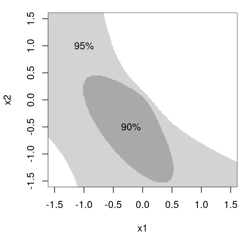

FIGURE 3.15: 90% and 95% confidence regions for stationary point \(x_s\).

Unfortunately, these confidence regions present a rather grim picture of the utility of our estimated stationary point. Although the smaller 90% region is clearly closed, and mostly contained with the study area, the larger 95% set doesn’t close inside the plot window which extends to cover the entirety of the experimental region. Recall the interpretation of a confidence set: that the true response surface maximum, which could reside at any location inside the (e.g., 95%) set, could readily have produced the data that were observed. Apparently, at the 95% level, that could be nearly any location nearby the design. (I leave it as an exercise to the curious reader to expand the grid and re-calculate the 95% region.) It’s perhaps surprising that we have such a high degree of uncertainty, even though our fit explains 84% of the variability in the response.

summary(fit)$r.squared

## [1] 0.8389

So as not to end on such a bleak message, consider a second dataset with the same design (so \(X^\top X\) is the same), but with a considerably better fit, explaining 99% of variability.

crdat$y <- c(87.6, 86.5, 85.7, 86.9, 86.7, 86.8, 87.4, 86.7, 90.3, 
  91.0, 90.8) 
fit2 <- lm(y ~ ., data=crdat)
summary(fit2)$r.squared

## [1] 0.9891

Updating the calculations from above with the new estimated coefficients …

b <- coef(fit)[2:3]
B <- matrix(NA, nrow=2, ncol=2)
diag(B) <- coef(fit)[4:5]
B[1,2] <- B[2,1] <- coef(fit)[6]/2
xs <- -(1/2)*solve(B, b)
s2 <- summary(fit2)$sigma^2
for(i in 1:nrow(g)) quadform[i] <- CIqf(g[i,1], g[i,2], s2, XtXi, b, B)

… leads to the 95% confidence region shown in Figure 3.16: a very compact set indeed.

ci95 <- quadform <= 2*qf(0.95, 2, nrow(X)-ncol(X))
image(xx, xx, matrix(ci95, ncol=length(xx)), xlab="x1", ylab="x2",
    col=c("white", "lightgray"))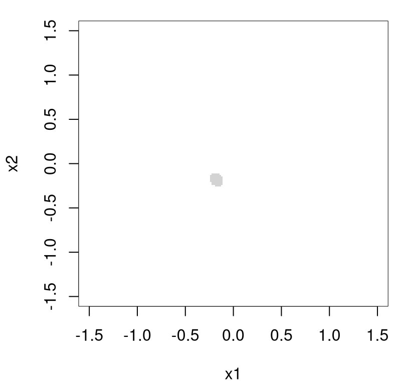

FIGURE 3.16: 95% confidence regions for stationary point \(x_s\) under higher \(R^2\); compare to Figure 3.15.

A smaller confidence region for the same level \(\alpha\) is a welcome result. It’s nice to have low ambiguity about where a local fit thinks best operating conditions lie, especially when the estimated \(x_s\) value is located within the design region. On the other hand, larger confidence regions are not always bad news. As in Figure 3.15, it’s possible for a model to fit quite well and yet generate a large confidence region. This state of affairs is merely a reflection of the reality that the response surface is locally flat. A positive spin may be that such situations imply a degree of flexibility in choosing the optimum. Communicating that effectively to stakeholders requires care, of course, but is definitely of interest.

3.2.5 Intervals on eigenvalues

In our discussion of the canonical analysis (§3.2.1) we noted that when one or more eigenvalues of \(B\) are close to zero a ridge system of some type is present. In judging the size of an eigenvalue it can be helpful to have a notion of standard error – to put some statistical heft behind just how small is basically zero. Standard errors can then be converted into CIs to ease reporting and interpretation.

A convenient procedure for developing standard errors for \(\lambda\), and subsequently CIs, is the double linear regression (DLR) method (Bisgaard and Ankenman 1996). As the name implies, it entails fitting two linear models. The first is a second-order model fit to data, as in any ridge analysis, providing the matrix \(B\) and its eigenvalues and vectors. The second is framed in the canonical model, whose so-called B-canonical form (3.4) we’ve used extensively throughout the latter half of this chapter. The DLR development instead utilizes an equivalent “A-canonical” form which is somewhat less common when studying ridge systems. The A-canonical form is based upon the representation \(\hat{y} = a_0 + u^\top a + u^\top \Lambda u\), where \(a = P^\top b\) and \(u = P^\top x\) with eigenvectors stacked in \(P\). Observe that the A-form utilizes axes rotated as in the B-form, but without translating from the stationary point \(x_s\) to the origin.

Rather than directly using \(a\) and \(\Lambda\)-values extracted from the eigen-analysis, they’re “re-inferred” through least squares on a design matrix of \(u\) and \(u^2\) predictors. Fitted values of that regression may be expressed as

\[ \hat{y} = \hat{a}_0 + \sum_{j=1}^m \hat{a}_j u_j + \sum_{j=1}^m \hat{\lambda}_j u_j^2. \]

Standard errors for \(\hat{\lambda}_j\) obtained in this way can be used to make \(100(1-\alpha)\)% CIs.

To illustrate, consider again the chemical processes experiment whose design is depicted in Figure 3.8. Code below duplicates some of our earlier effort to recreate variables pertinent to a ridge analysis, comprising the first regression in the DLR method.

chem <- read.table("chemical.txt", header=TRUE)
X <- data.frame(x1=chem$x1, x2=chem$x2, x11=chem$x1^2, x22=chem$x2^2, 
  x12=chem$x1*chem$x2)
y <- chem$y
fit <- lm(y ~ ., data=X)
b <- coef(fit)[2:3]
B <- matrix(NA, nrow=2, ncol=2)
diag(B) <- coef(fit)[4:5]
B[1,2] <- B[2,1] <- coef(fit)[6]/2
E <- eigen(B)
lambda <- E$values
o <- order(abs(lambda), decreasing=TRUE)
P <- E$vectors[,o]
print(lambda <- lambda[o])

## [1] -11.077  -2.673

Next derive \(u\) coordinates, following \(u = P^\top x\), and then expand out into second-order features (without interactions, since the system is already orthogonalized). Then fit the second regression involved in the DLR method.

U <- data.frame(cbind(chem$x1, chem$x2) %*% P)
names(U) <- c("u1", "u2")
U$u11 <- U$u1^2
U$u22 <- U$u2^2
fitU <- lm(y ~ ., data=U)

It’s not a coincidence that fitted coefficients from our canonical analysis match projected coefficients from the original model, and the eigenvalues.

rbind(dlr2=coef(fitU)[-1], eigen=c(b %*% P, lambda))

##           u1    u2    u11    u22
## dlr2  -10.81 2.126 -11.08 -2.673
## eigen -10.81 2.126 -11.08 -2.673

But now we can use summary.lm on the output of the second regression to extract standard errors on those eigenvalues.

summary(fitU)$coefficients[4:5,]

##     Estimate Std. Error t value  Pr(>|t|)
## u11  -11.077     0.9121 -12.144 5.868e-06
## u22   -2.673     0.9121  -2.931 2.200e-02

Observe that the \(t\)-tests provided in the table above, taken separately, reject the null hypothesis that \(\lambda_{4:5} = 0\). Therefore we conclude that both are indeed negative: the true response is a maximum. Alternatively, these standard errors can be used to construct CIs for the \(\lambda_j\)’s, or we can ask R to do it for us.

confint(fitU)[4:5,]

##      2.5 %  97.5 %
## u11 -13.23 -8.9201
## u22  -4.83 -0.5163

As expected, neither includes zero: both are squarely in the negative. We now have statistical evidence that the response surface is (locally) concave down, and can be reasonably confident that baby steps toward ascent will bear fruit.

Summarizing remarks

This concludes our chapter on classical response surface methods. Although barely scratching the surface, many of the underlying themes are present in abundance. In this careful enterprise there’s potential to learn a great deal, at least locally, from appropriately planned experiments. When conditions are right, a cautious ascent will likely lead to improvements. When they’re not, a statistical explanation can justify staying “right where you are” when little scope is apparent for incremental refinements to the process under study.

On the surface, it may seem that the biggest downside is the local nature of analysis. Another, perhaps more modern, perspective might suggest another drawback: reproducibility. Two different statistical experts might obtain dramatically different results or conclusions due to small changes or different choices (of design, size of ascent steps, etc.) along the way, despite being largely faithful to similar underlying principles. The process is far from automatable, which makes a meta-analysis, about what happens in the long run after repeatedly applying sequential procedures such as these, nearly impossible even in the abstract. Choice of design for convenience of analytical calculation, say in the calculation of confidence regions, may not be ideal either. Nevertheless, precedence for such tactics is well-established throughout academic statistics.

These drawbacks, local emphasis and removing expert variability toward machine automation, motivate much of what’s presented in subsequent chapters. Optimization and analysis of computer simulation experiments, nonlinear regression in spatial statistics and machine learning, are increasingly nonparametric. At first blush nonparametric methods seem more complex, and thus are often dismissed as black boxes. But that vastly oversimplifies a wide class of estimators. One clear positive side effect of non-parameter-“ism” is fewer choices requiring expert judgement, and therefore greater potential for automation and reproducibility. The canonical nonparametric apparatus in our setting is the Gaussian process. While no panacea, these remarkably agile beasts have already revolutionized scientific inquiry and optimization in the engineering and physical sciences, and deserve to be entertained as replacements to many well-established methods. Classical response surface methods are just one example.

3.3 Homework exercises

These exercises are designed to check your understanding of the method of steepest ascent, ridge analysis, and assessments of uncertainty thereupon. Data and parts of several questions are borrowed from Chapters 5–6 of Myers, Montgomery, and Anderson–Cook (2016), as detailed parenthetically below. Other exercises from those chapters come highly recommended.

#1: Steepest ascent

The file sadat.txt contains runs of an experiment on two input variables. (Synthesizes exercises 5.12, 5.24, and 5.25 from Myers, Montgomery, and Anderson–Cook (2016) using data from Table E5.602.)

1. Apply the method of steepest ascent and construct an appropriate path based on a first-order model. Report the path on both natural and coded variables.
2. Show graphically a confidence region for the path of steepest ascent. What fraction of the possible directions from the design origin are excluded by the path you computed in #a?
3. Perform tests for interaction and curvature. From these tests, do you feel comfortable engaging in the method of steepest ascent? Explain why or why not. Would you suggest any new runs besides those which are on the path from #a?

#2: Metallurgy

In a metallurgy experiment it’s desired to test the effect of four factors and their interactions on the concentration (percent by weight) of a particular phosphorus compound in casting material. The variables are: \(x_1\), percent phosphorus in the refinement; \(x_2\), percent remelted material; \(x_3\), fluxing time; and \(x_4\), holding time. The four factors are varied in a \(2^4\) factorial design with two castings taken at each factor combination. The 32 castings were made in random order, and are provided in metallurgy.txt, where the factors are presented in coded form. (Reproduced almost verbatim from exercise 5.5 in Myers, Montgomery, and Anderson–Cook (2016) using data from Table E5.601.)

1. Build a first-order response function.
2. Construct a table summarizing the path of steepest ascent in the coded design variables.
3. It’s important to constrain the percentages of phosphorus and remelted material. In fact, in coded variables we obtain \(x_1 + x_2 \leq 2.7\), where \(x_1\) is percent phosphorus and \(x_2\) is percent remelted material. Recalculate the path of steepest ascent subject to the above constraint.

#3: Heat transfer

In a chemical engineering experiment dealing with heat transfer in a shallow fluidized bed, data (in heat.txt) are collected on the following four regressor variables: fluidizing gas flow rate, lb/hr (fluid); supernatant gas flow rate, lb/hr (gas); supernatant gas inlet nozzle opening, mm (open); supernatant gas inlet temperature, °F (temp). The responses measured are heat transfer efficiency (heat) and thermal efficiency (therm). (Reproduced almost verbatim from exercise 6.2 in Myers, Montgomery, and Anderson–Cook (2016) using data from Table E6.1.)

This is a good example of what often happens in practice. An attempt was made to use a particular second-order design. However, errors in controlling the variables produced a design that’s only an approximation of the standard design.

1. Center and scale the design variables. That is, create a design matrix in coded form.
2. Fit a second-order model separately for both responses.
3. In the case of transfer efficiency (heat), do a canonical analysis and determine the nature of the stationary point. Do the same for thermal efficiency (therm).
4. For the case of transfer efficiency, what (natural) levels of the design variables would you recommend if maximum transfer efficiency is sought?
5. Do the same for thermal efficiency; that is, find levels of the design variables that you recommend for maximization of thermal efficiency.

#4: Bumper plating

A computer program simulates an auto-bumper plating process using thickness as the response with time, temperature (temp), and nickel pH as design variables. An experiment was conducted so that a response surface optimization could be entertained. A coding for the design variables is given by

\[ x_1 = \frac{\mbox{time} - 8}{4} \quad x_2 = \frac{\mbox{temp} - 24}{8} \quad x_3 = \frac{\mbox{nickel} - 14}{4}. \]

Using the data in bumper.txt, perform the following steps. (Inspired by exercise 6.9 in Myers, Montgomery, and Anderson–Cook (2016) using data from Table E6.6 which can be traced back to S. Schmidt and Launsby (1989).)

1. With the conversion above, write out the design matrix in coded form.
2. Fit and edit a second-order response surface model. That is, fit and eliminate insignificant terms.
3. Find conditions that maximize thickness, with the constraint that the condition falls inside the design region. In addition, compute the standard error for prediction at the location of optimum conditions.

#5: Gas turbine generators

The file turbine.txt contains runs of an experiment on two input variables, blade speed (in/sec) and voltage measuring sensor extension (in) describing the configuration of a gas turbine generator, and measuring the volts (voltage) output by the system. (Stripped down version of exercise 6.4 in Myers, Montgomery, and Anderson–Cook (2016) using data from Table E6.4.)

1. Write the design matrix in coded form.
2. Fit a second-order model, find the stationary point and interpret and visualize the fitted response surface.
3. Calculate and visualize a confidence region for the stationary point at the 90% and 95% levels. Approximately what proportion of those regions lie inside the design region?

#6: Viscosity

Consider an experiment summarized in viscosity.txt that studied a response triple (yield, viscosity and molecular weight molewt) as a function of two inputs, time and temperature (temp). For this question focus only on the viscosity output, ignoring the other two (yield and molewt). (Adapted from exercise 6.15 in Myers, Montgomery, and Anderson–Cook (2016) using data from Table E7.4.)

1. Perform a canonical analysis on the second-order model for these data.
2. Use the double linear regression method to find confidence intervals on the eigenvalues.
3. Interpret the fitted surface.

References

Bisgaard, S, and B Ankenman. 1996. “Standard Errors for the Eigenvalues in Second-Order Response Surface Models.” Technometrics 38 (3): 238–46.

Draper, NR. 1963. “Ridge Analysis of Response Surfaces.” Technometrics 5 (4): 469–79.

Myers, RH, DC Montgomery, and CM Anderson–Cook. 2016. Response Surface Methodology: Process and Product Optimization Using Designed Experiments. John Wiley & Sons.

Schmidt, SR, and RG Launsby. 1989. Understanding Industrial Designed Experiments. Air Academy Press.