Chapter 5 Gaussian Process Regression
Here the goal is humble on theoretical fronts, but fundamental in application. Our aim is to understand the Gaussian process (GP) as a prior over random functions, a posterior over functions given observed data, as a tool for spatial data modeling and surrogate modeling for computer experiments, and simply as a flexible nonparametric regression. We’ll see that, almost in spite of a technical over-analysis of its properties, and sometimes strange vocabulary used to describe its features, GP regression is a simple extension of linear modeling. Knowing that is all it takes to make use of it as a nearly unbeatable regression tool when input–output relationships are relatively smooth, and signal-to-noise ratios relatively high. And even sometimes when they’re not.
The subject of this chapter goes by many names and acronyms. Some call it kriging, which is a term that comes from geostatistics (Matheron 1963); some call it Gaussian spatial modeling or a Gaussian stochastic process. Both, if you squint at them the right way, have the acronym GaSP. Machine learning (ML) researchers like Gaussian process regression (GPR). All of these instances are about regression: training on inputs and outputs with the ultimate goal of prediction and uncertainty quantification (UQ), and ancillary goals that are either tantamount to, or at least crucially depend upon, qualities and quantities derived from a predictive distribution. Although the chapter is titled “Gaussian process regression”, and we’ll talk lots about Gaussian process surrogate modeling throughout this book, we’ll typically shorten that mouthful to Gaussian process (GP), or use “GP surrogate” for short. GPS would be confusing and GPSM is too scary. I’ll try to make this as painless as possible.
After understanding how it all works, we’ll see how GPs excel in several common response surface tasks: as a sequential design tool in Chapter 6; as the workhorse in modern (Bayesian) optimization of blackbox functions in Chapter 7; and all that with a “hands off” approach. Classical RSMs of Chapter 3 have many attractive features, but most of that technology was designed specifically, and creatively, to cope with limitations arising in first- and second-order linear modeling. Once in the more flexible framework that GPs provide, one can think big without compromising finer detail on smaller things.
Of course GPs are no panacea. Specialized tools can work better in less generic contexts. And GPs have their limitations. We’ll have the opportunity to explore just what they are, through practical examples. And down the line in Chapter 9 we’ll see that most of those are easy to sweep away with a bit of cunning. These days it’s hard to make the case that a GP shouldn’t be involved as a component in a larger analysis, or at least attempted as such, where ultimately limited knowledge of the modeling context can be met by a touch of flexibility, taking us that much closer to human-free statistical “thinking” – a fundamental desire in ML and thus, increasingly, in tools developed for modern analytics.
5.1 Gaussian process prior
Gaussian process is a generic term that pops up, taking on disparate but quite specific meanings, in various statistical and probabilistic modeling enterprises. As a generic term, all it means is that any finite collection of realizations (i.e., \(n\) observations) is modeled as having a multivariate normal (MVN) distribution. That, in turn, means that characteristics of those realizations are completely described by their mean \(n\)-vector \(\mu\) and \(n \times n\) covariance matrix \(\Sigma\). With interest in modeling functions, we’ll sometimes use the term mean function, thinking of \(\mu(x)\), and covariance function, thinking of \(\Sigma(x, x')\). But ultimately we’ll end up with vectors \(\mu\) and matrices \(\Sigma\) after evaluating those functions at specific input locations \(x_1, \dots, x_n\).
You’ll hear people talk about function spaces, reproducing kernel Hilbert spaces, and so on, in the context of GP modeling of functions. Sometimes thinking about those aspects/properties is important, depending on context. For most purposes that makes things seem fancier than they really need to be.
The action, at least the part that’s interesting, in a GP treatment of functions is all in the covariance. Consider a covariance function defined by inverse exponentiated squared Euclidean distance:
\[ \Sigma(x, x') = \exp\{ - || x - x '||^2 \}. \]
Here covariance decays exponentially fast as \(x\) and \(x'\) become farther apart in the input, or \(x\)-space. In this specification, observe that \(\Sigma(x,x) = 1\) and \(\Sigma(x, x') < 1\) for \(x' \ne x\). The function \(\Sigma(x, x')\) must be positive definite. For us this means that if we define a covariance matrix \(\Sigma_n\), based on evaluating \(\Sigma(x_i, x_j\)) at pairs of \(n\) \(x\)-values \(x_1, \dots, x_n\), we must have that
\[ x^\top \Sigma_n x > 0 \quad \mbox{ for all } x \ne 0. \]
We intend to use \(\Sigma_n\) as a covariance matrix in an MVN, and a positive (semi-) definite covariance matrix is required for MVN analysis. In that context, positive definiteness is the multivariate extension of requiring that a univariate Gaussian have positive variance parameter, \(\sigma^2\).
To ultimately see how a GP with that simple choice of covariance \(\Sigma_n\) can be used to perform regression, let’s first see how GPs can be used to generate random data following a smooth functional relationship. Suppose we take a bunch of \(x\)-values: \(x_1,\dots, x_n\), define \(\Sigma_n\) via \(\Sigma_n^{ij} = \Sigma(x_i, x_j)\), for \(i,j=1,\dots,n\), then draw an \(n\)-variate realization
\[ Y \sim \mathcal{N}_n(0, \Sigma_n), \]
and plot the result in the \(x\)-\(y\) plane. That was a mouthful, but don’t worry: we’ll see it in code momentarily. First note that the mean of this MVN is zero; this need not be but it’s quite surprising how well things work even in this special case. Location invariant zero-mean GP modeling, sometimes after subtracting off a middle value of the response (e.g., \(\bar{y}\)), is the default in computer surrogate modeling and (ML) literatures. We’ll talk about generalizing this later.
Here’s a version of that verbal description with \(x\)-values in 1d. First create an input grid with 100 elements.
Next calculate pairwise squared Euclidean distances between those inputs. I like the distance function from the plgp package (Gramacy 2014) in R because it was designed exactly for this purpose (i.e., for use with GPs), however dist in base R provides similar functionality.
Then build up covariance matrix \(\Sigma_n\) as inverse exponentiated squared Euclidean distances. Notice that the code below augments the diagonal with a small number eps \(\equiv \epsilon\). Although inverse exponentiated distances guarantee a positive definite matrix in theory, sometimes in practice the matrix is numerically ill-conditioned. Augmenting the diagonal a tiny bit prevents that. Neal (1998), a GP vanguard in the statistical/ML literature, calls \(\epsilon\) the jitter in this context.
Finally, plug that covariance matrix into an MVN random generator; below I use one from the mvtnorm package (Genz et al. 2018) on CRAN.
That’s it! We’ve generated a finite realization of a random function under a GP prior with a particular covariance structure. Now all that’s left is visualization. Figure 5.1 plots those X and Y pairs as tiny connected line segments on an \(x\)-\(y\) plane.

FIGURE 5.1: A random function under a GP prior.
Because the \(Y\)-values are random, you’ll get a different curve when you try this on your own. We’ll generate some more below in a moment. But first, what are the properties of this function, or more precisely of a random function generated in this way? Several are easy to deduce from the form of the covariance structure. We’ll get a range of about \([-2,2]\), with 95% probability, because the scale of the covariance is 1, ignoring the jitter \(\epsilon\) added to the diagonal. We’ll get several bumps in the \(x\)-range of \([0,10]\) because short distances are highly correlated (about 37%) and long distances are essentially uncorrelated (\(1e^{-7}\)).
## [1] 3.679e-01 1.125e-07Now the function plotted above is only a finite realization, meaning that we really only have 100 pairs of points. Those points look smooth, in a tactile sense, because they’re close together and because the plot function is “connecting the dots” with lines. The full surface, which you might conceptually extend to an infinite realization over a compact domain, is extremely smooth in a calculus sense because the covariance function is infinitely differentiable, a discussion we’ll table for a little bit later.
Besides those three things – scale of two, several bumps, smooth look – we won’t be able to anticipate much else about the nature of a particular realization. Figure 5.2 shows three new random draws obtained in a similar way, which will again look different when you run the code on your own.
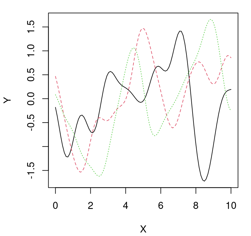
FIGURE 5.2: Three more random functions under a GP prior.
Each random finite collection is different than the next. They all have similar range, about the same number of bumps, and are smooth. That’s what it means to have function realizations under a GP prior: \(Y(x) \sim \mathcal{GP}\).
5.1.1 Gaussian process posterior
Of course, we’re not in the business of generating random functions. I’m not sure what that would be useful for. Instead, we ask: given examples of a function in pairs \((x_1, y_1), \dots, (x_n, y_n)\), comprising data \(D_n = (X_n, Y_n)\), what random function realizations could explain – could have generated – those observed values? That is, we want to know about the conditional distribution of \(Y(x) \mid D_n\). If we call \(Y(x) \sim \mathcal{GP}\) the prior, then \(Y(x) \mid D_n\) must be the posterior.
Fortunately, you don’t need to be a card-carrying Bayesian to appreciate what’s going on, although that perspective has really taken hold in ML. That conditional distribution, \(Y(x) \mid D_n\), which one might more simply call a predictive distribution, is a familiar quantity in regression analysis. Forget for the moment that when regressing one is often interested in other aspects, like relevance of predictors through estimates of parameter standard errors, etc., and that so far our random functions look like they have no noise. The somewhat strange, and certainly most noteworthy, thing is that so far there are no parameters!
Let’s shelve interpretation (Bayesian updating or a twist on simple regression) for a moment and focus on conditional distributions, because that’s what it’s really all about. Deriving that predictive distribution is a simple application of deducing a conditional from a (joint) MVN. From Wikipedia, if an \(N\)-dimensional random vector \(X\) is partitioned as
\[ X = \left( \begin{array}{c} X_1 \\ X_2 \end{array} \right) \quad \mbox{ with sizes } \quad \left( \begin{array}{c} q \times 1 \\ (N-q) \times 1 \end{array} \right), \]
and accordingly \(\mu\) and \(\Sigma\) are partitioned as,
\[ \mu = \left( \begin{array}{c} \mu_1 \\ \mu_2 \end{array} \right) \quad \mbox{ with sizes } \quad \left( \begin{array}{c} q \times 1 \\ (N-q) \times 1 \end{array} \right) \]
and
\[ \Sigma = \left(\begin{array}{cc} \Sigma_{11} & \Sigma_{12} \\ \Sigma_{21} & \Sigma_{22} \end{array} \right) \ \mbox{ with sizes } \ \left(\begin{array}{cc} q \times q & q \times (N-q) \\ (N-q)\times q & (N - q)\times (N-q) \end{array} \right), \]
then the distribution of \(X_1\) conditional on \(X_2 = x_2\) is MVN \(X_1 \mid x_2 \sim \mathcal{N}_q (\bar{\mu}, \bar{\Sigma})\), where
\[\begin{align} \bar{\mu} &= \mu_1 + \Sigma_{12} \Sigma_{22}^{-1}(x_2 - \mu_2) \tag{5.1} \\ \mbox{and } \quad \bar{\Sigma} &= \Sigma_{11} - \Sigma_{12} \Sigma_{22}^{-1} \Sigma_{21}. \notag \end{align}\]
An interesting feature of this result is that conditioning upon \(x_2\) alters the variance of \(X_1\). Observe that \(\bar{\Sigma}\) above is reduced compared to its marginal analog \(\Sigma_{11}\). Reduction in variance when conditioning on data is a hallmark of statistical learning. We know more – have less uncertainty – after incorporating data. Curiously, the amount by which variance is decreased doesn’t depend on the value of \(x_2\). Observe that the mean is also altered, comparing \(\mu_1\) to \(\bar{\mu}\). In fact, the equation for \(\bar{\mu}\) is a linear mapping, i.e., of the form \(ax + b\) for vectors \(a\) and \(b\). Finally, note that \(\Sigma_{12} = \Sigma_{21}^\top\) so that \(\bar{\Sigma}\) is symmetric.
Ok, how do we deploy that fundamental MVN result towards deriving the GP predictive distribution \(Y(x) \mid D_n\)? Consider an \(n+1^{\mathrm{st}}\) observation \(Y(x)\). Allow \(Y(x)\) and \(Y_n\) to have a joint MVN distribution with mean zero and covariance function \(\Sigma(x,x')\). That is, stack
\[ \left( \begin{array}{c} Y(x) \\ Y_n \end{array} \right) \quad \mbox{ with sizes } \quad \left( \begin{array}{c} 1 \times 1 \\ n \times 1 \end{array} \right), \]
and if \(\Sigma(X_n,x)\) is the \(n \times 1\) matrix comprised of \(\Sigma(x_1, x), \dots, \Sigma(x_n, x)\), its covariance structure can be partitioned as follows:
\[ \left(\begin{array}{cc} \Sigma(x,x) & \Sigma(x,X_n) \\ \Sigma(X_n,x) & \Sigma_n \end{array} \right) \ \mbox{ with sizes } \ \left(\begin{array}{cc} 1 \times 1 & 1 \times n \\ n\times 1 & n \times n \end{array} \right). \]
Recall that \(\Sigma(x,x) = 1\) with our simple choice of covariance function, and that symmetry provides \(\Sigma(x,X_n) = \Sigma(X_n,x)^\top\).
Applying Eq. (5.1) yields the following predictive distribution
\[ Y(x) \mid D_n \sim \mathcal{N}(\mu(x), \sigma^2(x)) \]
with
\[\begin{align} \mbox{mean } \quad \mu(x) &= \Sigma(x, X_n) \Sigma_n^{-1} Y_n \tag{5.2} \\ \mbox{and variance } \quad \sigma^2(x) &= \Sigma(x,x) - \Sigma(x, X_n) \Sigma_n^{-1} \Sigma(X_n, x). \notag \end{align}\]
Observe that \(\mu(x)\) is linear in observations \(Y_n\), so we have a linear predictor! In fact it’s the best linear unbiased predictor (BLUP), an argument we’ll leave to other texts (e.g., Santner, Williams, and Notz 2018). Also notice that \(\sigma^2(x)\) is lower than the marginal variance. So we learn something from data \(Y_n\); in fact the amount that variance goes down is a quadratic function of distance between \(x\) and \(X_n\). Learning is most efficient for \(x\) that are close to training data locations \(X_n\). However the amount learned doesn’t depend upon \(Y_n\). We’ll return to that later.
The derivation above is for “pointwise” GP predictive calculations. These are sometimes called the kriging equations, especially in geospatial contexts. We can apply them, separately, for many predictive/testing locations \(x\), one \(x\) at a time, but that would ignore the obvious correlation they’d experience in a big MVN analysis. Alternatively, we may consider a bunch of \(x\) locations jointly, in a testing design \(\mathcal{X}\) of \(n'\) rows, say, all at once:
\[ Y(\mathcal{X}) \mid D_n \sim \mathcal{N}_{n'}(\mu(\mathcal{X}), \Sigma(\mathcal{X})) \]
with
\[\begin{align} \mbox{mean } \quad \mu(\mathcal{X}) &= \Sigma(\mathcal{X}, X_n) \Sigma_n^{-1} Y_n \tag{5.3}\\ \mbox{and variance } \quad \Sigma(\mathcal{X}) &= \Sigma(\mathcal{X},\mathcal{X}) - \Sigma(\mathcal{X}, X_n) \Sigma_n^{-1} \Sigma(\mathcal{X}, X_n)^\top, \notag \end{align}\]
where \(\Sigma(\mathcal{X}, X_n)\) is an \(n' \times n\) matrix. Having a full covariance structure offers a more complete picture of the random functions which explain data under a GP posterior, but also more computation. The \(n' \times n'\) matrix \(\Sigma(\mathcal{X})\) could be enormous even for seemingly moderate \(n'\).
Simple 1d GP prediction example
Consider a toy example in 1d where the response is a simple sinusoid measured at eight equally spaced \(x\)-locations in the span of a single period of oscillation. R code below provides relevant data quantities, including pairwise squared distances between the input locations collected in the matrix D, and its inverse exponentiation in Sigma.
n <- 8
X <- matrix(seq(0, 2*pi, length=n), ncol=1)
y <- sin(X)
D <- distance(X)
Sigma <- exp(-D) + diag(eps, ncol(D))
Now this is where the example diverges from our earlier one, where we used such quantities to generate data from a GP prior. Applying MVN conditioning equations requires similar calculations on a testing design \(\mathcal{X}\), coded as XX below. We need inverse exponentiated squared distances between those XX locations …
XX <- matrix(seq(-0.5, 2*pi + 0.5, length=100), ncol=1)
DXX <- distance(XX)
SXX <- exp(-DXX) + diag(eps, ncol(DXX))
… as well as between testing locations \(\mathcal{X}\) and training data locations \(X_n\).
Note that an \(\epsilon\) jitter adjustment is not required for SX because it need not be decomposed in the conditioning calculations (and SX is anyways not square). We do need jitter on the diagonal of SXX though, because this matrix is directly involved in calculation of the predictive covariance which we shall feed into an MVN generator below.
Now simply follow Eq. (5.3) to derive joint predictive equations for XX \(\equiv \mathcal{X}\): invert \(\Sigma_n\), apply the linear predictor, and calculate reduction in covariance.
Above mup maps to \(\mu(\mathcal{X})\) evaluated at our testing grid \(\mathcal{X} \equiv\) XX, and Sigmap similarly for \(\Sigma(\mathcal{X})\) via pairs in XX. As a computational note, observe that Siy <- Si %*% y may be pre-computed in time quadratic in \(n=\) length(y) so that mup may subsequently be calculated for any XX in time linear in \(n\), without redoing Siy; for example, as solve(Sigma, y). There are two reasons we’re not doing that here. One is to establish a clean link between code and mathematical formulae. The other is a presumption that the variance calculation, which remains quadratic in \(n\) no matter what, is at least as important as the mean.
Mean vector and covariance matrix in hand, we may generate \(Y\)-values from the posterior/predictive distribution \(Y(\mathcal{X}) \mid D_n\) in the same manner as we did from the prior.
Those \(Y(\mathcal{X}) \equiv\) YY samples may then be plotted as a function of predictive input \(\mathcal{X} \equiv\) XX locations. Before doing that, extract some pointwise quantile-based error-bars from the diagonal of \(\Sigma(\mathcal{X})\) to aid in visualization.
Figure 5.3 plots each of the random predictive, finite realizations as gray curves. Training data points are overlayed, along with true response at the \(\mathcal{X}\) locations as a thin blue line. Predictive mean \(\mu(\mathcal{X})\) in black, and 90% quantiles in dashed-red, are added as thicker lines.
matplot(XX, t(YY), type="l", col="gray", lty=1, xlab="x", ylab="y")
points(X, y, pch=20, cex=2)
lines(XX, sin(XX), col="blue")
lines(XX, mup, lwd=2)
lines(XX, q1, lwd=2, lty=2, col=2)
lines(XX, q2, lwd=2, lty=2, col=2)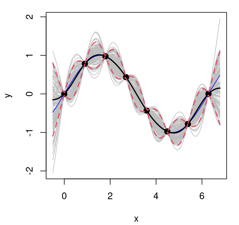
FIGURE 5.3: Posterior predictive distribution in terms of means (solid black), quantiles (dashed-red), and draws (gray). The truth is shown as a thin blue line.
What do we observe in the figure? Notice how the predictive surface interpolates the data. That’s because \(\Sigma(x, x) = 1\) and \(\Sigma(x, x') \rightarrow 1^-\) as \(x' \rightarrow x\). Error-bars take on a “football” shape, or some say a “sausage” shape, being widest at locations farthest from \(x_i\)-values in the data. Error-bars get really big outside the range of the data, a typical feature in ordinary linear regression settings. But the predictive mean behaves rather differently than under an ordinary linear model. For GPs it’s mean-reverting, eventually leveling off to zero as \(x \in \mathcal{X}\) gets far away from \(X_n\). Predictive variance, as exemplified by those error-bars, is also reverting to something: a prior variance of 1. In particular, variance won’t continue to increase as \(x\) gets farther and farther from \(X_n\). Together those two “reversions” imply that although we can’t trust extrapolations too far outside of the data range, at least their behavior isn’t unpredictable, as can sometimes happen in linear regression contexts, for example when based upon feature-expanded (e.g., polynomial basis) covariates.
These characteristics, especially the football/sausage shape, is what makes GPs popular as surrogates for computer simulation experiments. That literature, which historically emphasized study of deterministic computer simulators, drew comfort from interpolation-plus-expansion of variance away from training simulations. Perhaps more importantly, they liked that out-of-sample prediction was highly accurate. Come to think of it, that’s why spatial statisticians and machine learners like them too. But hold that thought; there are a few more things to do before we get to predictive comparisons.
5.1.2 Higher dimension?
There’s nothing particularly special about the presentation above that would preclude application in higher input dimension. Except perhaps that visualization is a lot simpler in 1d or 2d. We’ll get to even higher dimensions with some of our later examples. For now, consider a random function in 2d sampled from a GP prior. The plan is to go back through the process above: first prior, then (posterior) predictive, etc.
Begin by creating an input set, \(X_n\), in two dimensions. Here we’ll use a regular \(20 \times 20\) grid.
Then calculate pairwise distances and evaluate covariances under inverse exponentiated squared Euclidean distances, plus jitter.
Finally make random MVN draws in exactly the same way as before. Below we save two such draws.
For visualization in Figure 5.4, persp is used to stretch each \(20 \times 20\) = 400-variate draw over a mesh with a fortuitously chosen viewing angle.
par(mfrow=c(1,2))
persp(x, x, matrix(Y[1,], ncol=nx), theta=-30, phi=30, xlab="x1",
ylab="x2", zlab="y")
persp(x, x, matrix(Y[2,], ncol=nx), theta=-30, phi=30, xlab="x1",
ylab="x2", zlab="y")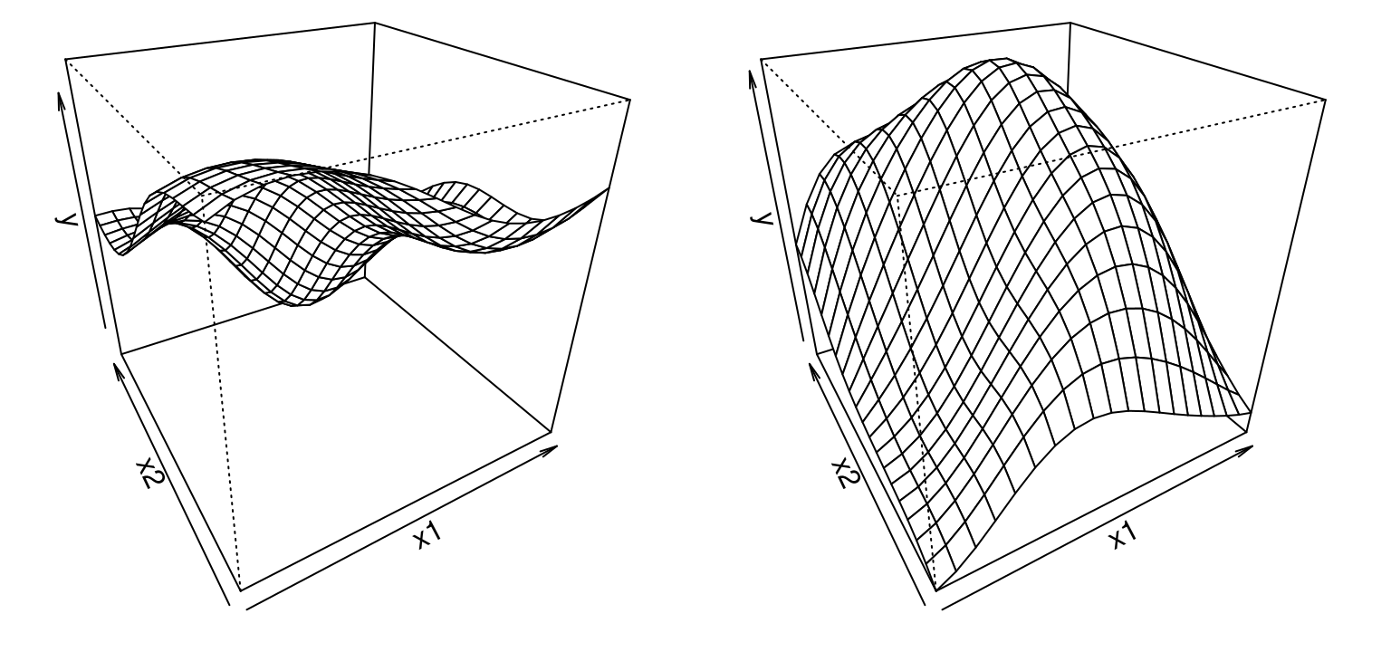
FIGURE 5.4: Two random functions under a GP prior in 2d.
So drawing from a GP prior in 2d is identical to the 1d case, except with a 2d input grid. All other code is “cut-and-paste”. Visualization is more cumbersome, but that’s a cosmetic detail. Learning from training data, i.e., calculating the predictive distribution for observed \((x_i, y_i)\) pairs, is no different: more cut-and-paste.
To try it out we need to cook up some toy data from which to learn. Consider the 2d function \(y(x) = x_1 \exp\{-x_1^2 - x_2^2\}\) which is highly nonlinear near the origin, but flat (zero) as inputs get large. This function has become a benchmark 2d problem in the literature for reasons that we’ll get more into in Chapter 9. Suffice it to say that thinking up simple-yet-challenging toy problems is a great way to get noticed in the community, even when you borrow a common example in vector calculus textbooks or one used to demonstrate 3d plotting features in MATLAB®.
library(lhs)
X <- randomLHS(40, 2)
X[,1] <- (X[,1] - 0.5)*6 + 1
X[,2] <- (X[,2] - 0.5)*6 + 1
y <- X[,1]*exp(-X[,1]^2 - X[,2]^2)Above, a Latin hypercube sample (LHS; §4.1) is used to generate forty (coded) input locations in lieu of a regular grid in order to create a space-filling input design. A regular grid with 400 elements would have been overkill, but a uniform random design of size forty or so would have worked equally well. Coded inputs are mapped onto a scale of \([-2,4]^2\) in order to include both bumpy and flat regions.
Let’s suppose that we wish to interpolate those forty points onto a regular \(40 \times 40\) grid, say for stretching over a mesh. Here’s code that creates such testing locations XX \(\equiv\mathcal{X}\) in natural units.
Now that we have inputs and outputs, X and y, and predictive locations XX we can start cutting-and-pasting. Start with the relevant training data quantities …
… and follow with similar calculations between input sets X and XX.
Then apply Eq. (5.3). Code wise, these lines are identical to what we did in the 1d case.
It’s hard to visualize a multitude of sample paths in 2d – two was plenty when generating from the prior – but if desired, we may obtain them with the same rmvnorm commands as in §5.1.1. Instead focus on plotting pointwise summaries, namely predictive mean \(\mu(x) \equiv\) mup and predictive standard deviation \(\sigma(x)\):
The left panel in Figure 5.5 provides an image plot of the mean over our regularly-gridded inputs XX; the right panel shows standard deviation.
par(mfrow=c(1,2))
cols <- heat.colors(128)
image(xx, xx, matrix(mup, ncol=length(xx)), xlab="x1", ylab="x2", col=cols)
points(X[,1], X[,2])
image(xx, xx, matrix(sdp, ncol=length(xx)), xlab="x1", ylab="x2", col=cols)
points(X[,1], X[,2])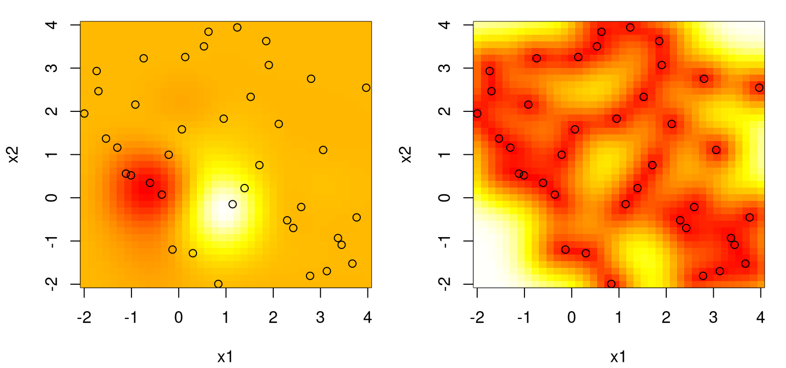
FIGURE 5.5: Posterior predictive for a two-dimensional example, via mean (left) and standard deviation (right) surfaces. Training data input locations are indicated by open circles.
What do we observe? Pretty much the same thing as in the 1d case. We can’t see it, but the predictive surface interpolates. Predictive uncertainty, here as standard deviation \(\sigma(x)\), is highest away from \(x_i\)-values in the training data. Predictive intervals don’t look as much like footballs or sausages, yet somehow that analogy still works. Training data locations act as anchors to smooth variation between points with an organic rise in uncertainty as we imagine predictive inputs moving away from one toward the next.
Figure 5.6 provides another look, obtained by stretching the predictive mean over a mesh. Bumps near the origin are clearly visible, with a flat region emerging for larger \(x_1\) and \(x_2\) settings.
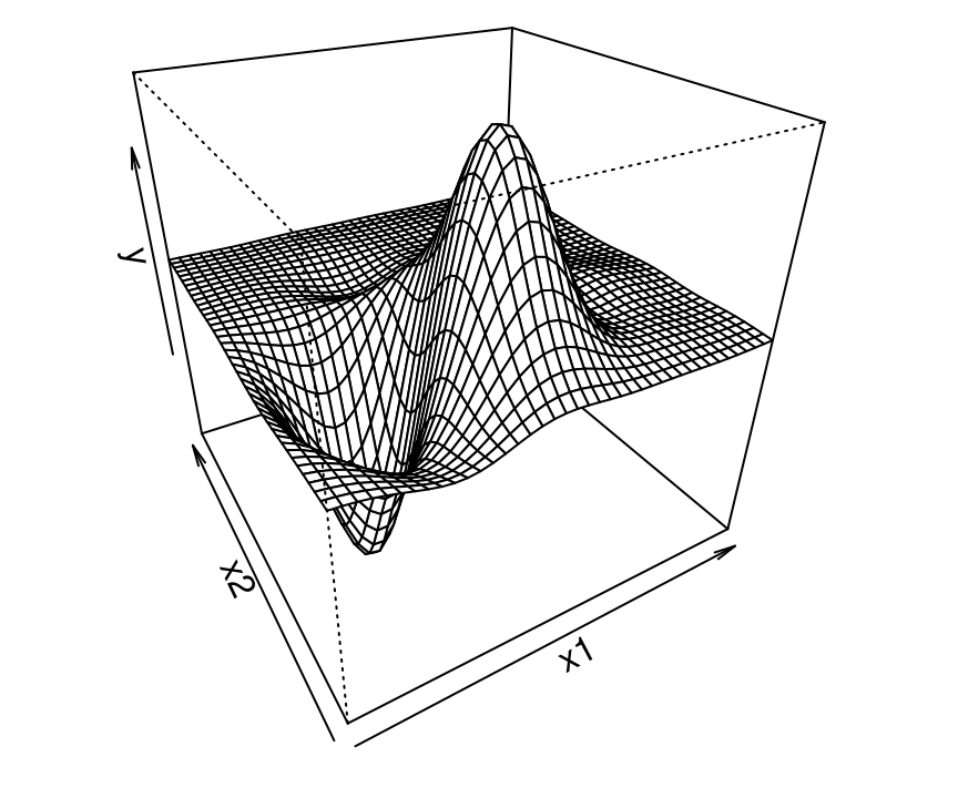
FIGURE 5.6: Perspective view on the posterior mean surface from the left panel of Figure 5.5.
Well that’s basically it! Now you know GP regression. Where to go from here? Hopefully I’ve convinced you that GPs hold great potential as a nonlinear regression tool. It’s kinda-cool that they perform so well – that they “learn” – without having to tune anything. In statistics, we’re so used to seeking out optimal settings of parameters that a GP predictive surface might seem like voodoo. Simple MVN conditioning is able to capture input–output dynamics without having to “fit” anything, or without trying to minimize a loss criteria. That flexibility, without any tuning knobs, is what people think of when they call GPs a nonparametric regression tool. All we did was define covariance in terms of (inverse exponentiated squared Euclidean) distance, condition, and voilà.
But when you think about it a little bit, there are lots of (hidden) assumptions which are going to be violated by most real-data contexts. Data is noisy. The amplitude of all functions we might hope to learn will not be 2. Correlation won’t decay uniformly in all directions, i.e., radially. Even the most ideally smooth physical relationships are rarely infinitely smooth.
Yet we’ll see that even gross violations of those assumptions are easy to address, or “fix up”. At the same time GPs are relatively robust to transgressions between assumptions and reality. In other words, sometimes it works well even when it ought not. As I see it – once we clean things up – there are really only two serious problems that GPs face in practice: stationarity of covariance (§5.3.3), and computational burden, which in most contexts go hand-in-hand. Remedies for both will have to wait for Chapter 9. For now, let’s keep the message upbeat. There’s lots that can be accomplished with the canonical setup, whose description continues below.
5.2 GP hyperparameters
All this business about nonparametric regression and here we are introducing parameters, passive–aggressively you might say: refusing to call them parameters. How can one have hyperparameters without parameters to start with, or at least to somehow distinguish from? To make things even more confusing, we go about learning those hyperparameters in the usual way, by optimizing something, just like parameters. I guess it’s all to remind you that the real power – the real flexibility – comes from MVN conditioning. These hyperparameters are more of a fine tuning. There’s something to that mindset, as we shall see. Below we revisit the drawbacks alluded to above – scale, noise, and decay of correlation – with a (fitted) hyperparameter targeting each one.
5.2.1 Scale
Suppose you want your GP prior to generate random functions with an amplitude larger than two. You could introduce a scale parameter \(\tau^2\) and then take \(\Sigma_n = \tau^2 C_n\). Here \(C\) is basically the same as our \(\Sigma\) from before: a correlation function for which \(C(x,x) = 1\) and \(C(x,x') < 1\) for \(x \ne x'\), and positive definite; for example
\[ C(x, x') = \exp \{- || x - x' ||^2 \}. \]
But we need a more nuanced notion of covariance to allow more flexibility on scale, so we’re re-parameterizing a bit. Now our MVN generator looks like
\[ Y \sim \mathcal{N}_n(0, \tau^2 C_n). \]
Let’s check that that does the trick. First rebuild \(X_n\)-locations, e.g., a sequence of one hundred from zero to ten, and then calculate pairwise distances. Nothing different yet compared to our earlier illustration in §5.1.
Now amplitude, via 95% of the range of function realizations, is approximately \(2\sigma(x)\) where \(\sigma^2 \equiv \mathrm{diag}(\Sigma_n)\). So for an amplitude of 10, say, choose \(\tau^2 = 5^2 = 25\). The code below calculates inverse exponentiated squared Euclidean distances in \(C_n\) and makes ten draws from an MVN whose covariance is obtained by pre-multiplying \(C_n\) by \(\tau^2\).
As Figure 5.7 shows, amplitude has increased. Not all draws completely lie between \(-10\) and \(10\), but most are in the ballpark.
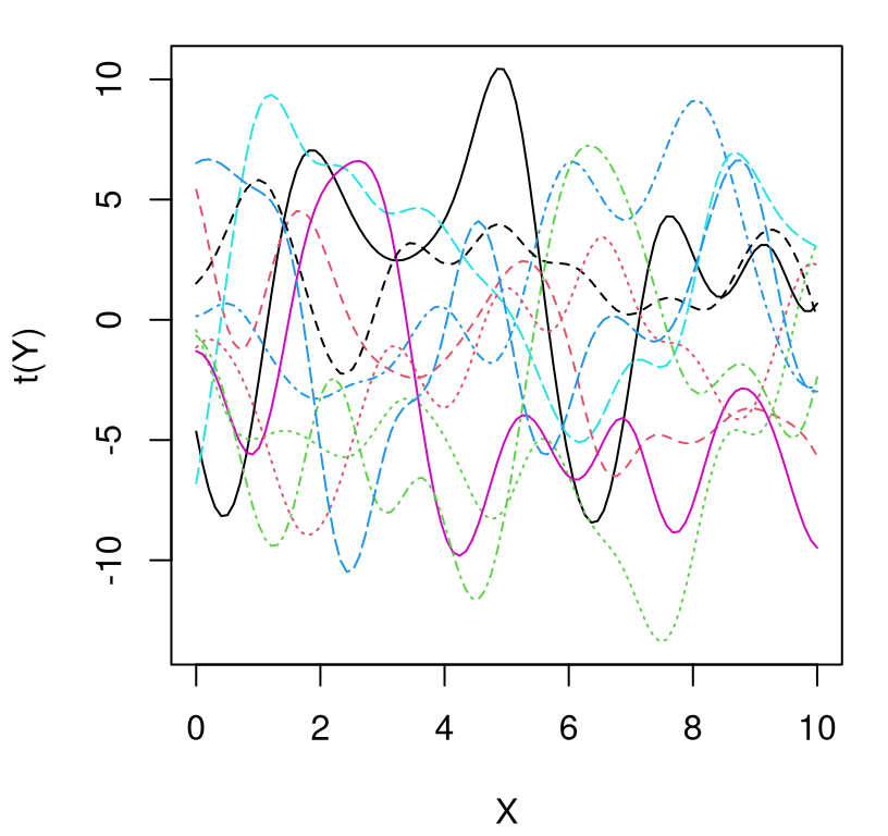
FIGURE 5.7: Higher amplitude draws from a GP prior.
But again, who cares about generating random functions? We want to be able to learn about functions on any scale from training data. What would happen if we had some data with an amplitude of 5, say, but we used a GP with a built-in scale of 1 (amplitude of 2). In other words, what would happen if we did things the “old-fashioned way”, with code cut-and-pasted directly from §5.1.1?
First generate some data with that property. Here we’re revisiting sinusoidal data from §5.1.1, but multiplying by 5 on the way out of the sin call.
Next cut-and-paste code from earlier, including our predictive grid of 100 equally spaced locations.
D <- distance(X)
Sigma <- exp(-D)
XX <- matrix(seq(-0.5, 2*pi + 0.5, length=100), ncol=1)
DXX <- distance(XX)
SXX <- exp(-DXX) + diag(eps, ncol(DXX))
DX <- distance(XX, X)
SX <- exp(-DX)
Si <- solve(Sigma);
mup <- SX %*% Si %*% y
Sigmap <- SXX - SX %*% Si %*% t(SX)Now we have everything we need to visualize the resulting predictive surface, which is shown in Figure 5.8 using plotting code identical to that behind Figure 5.3.
YY <- rmvnorm(100, mup, Sigmap)
q1 <- mup + qnorm(0.05, 0, sqrt(diag(Sigmap)))
q2 <- mup + qnorm(0.95, 0, sqrt(diag(Sigmap)))
matplot(XX, t(YY), type="l", col="gray", lty=1, xlab="x", ylab="y")
points(X, y, pch=20, cex=2)
lines(XX, mup, lwd=2)
lines(XX, 5*sin(XX), col="blue")
lines(XX, q1, lwd=2, lty=2, col=2)
lines(XX, q2, lwd=2, lty=2, col=2)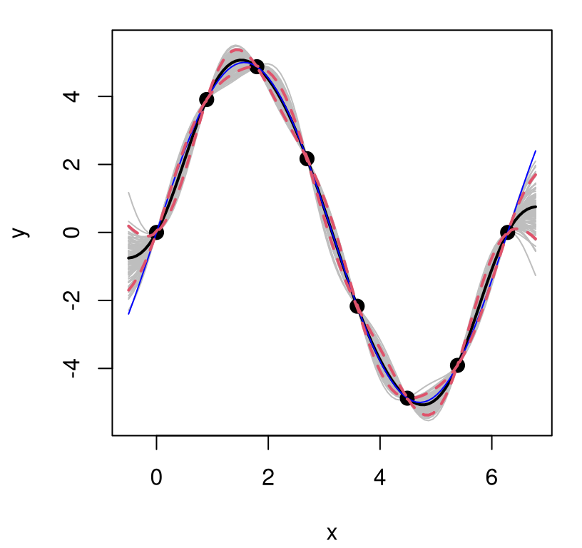
FIGURE 5.8: GP fit to higher amplitude sinusoid.
What happened? In fact the “scale 1” GP is pretty robust. It gets the predictive mean almost perfectly, despite using the “wrong prior” relative to the actual data generating mechanism, at least as regards scale. But it’s over-confident. Besides a change of scale, the new training data exhibit no change in relative error, nor any other changes for that matter, compared to the example we did above where the scale was actually 1. So we must now be under-estimating predictive uncertainty, which is obvious by visually comparing the error-bars to those obtained from our earlier fit (Figure 5.3). Looking closely, notice that the true function goes well outside of our predictive interval at the edges of the input space. That didn’t happen before.
How to estimate the right scale? Well for starters, admit that scale may be captured by a parameter, \(\tau^2\), even though we’re going to call it a hyperparameter to remind ourselves that its impact on the overall estimation procedure is really more of a fine-tuning. The analysis above lends some credence to that perspective, since our results weren’t too bad even though we assumed an amplitude that was off by a factor of five. Whether benevolently gifted the right scale or not, GPs clearly retain a great deal of flexibility to adapt to the dynamics at play in data. Decent predictive surfaces often materialize, as we have seen, in spite of less than ideal parametric specifications.
As with any “parameter”, there are many choices when it comes to estimation: method of moments (MoM), likelihood (maximum likelihood, Bayesian inference), cross validation (CV), the “eyeball norm”. Some, such as those based on (semi-) variograms, are preferred in the spatial statistics literature. All of those are legitimate, except maybe the eyeball norm which isn’t very easily automated and challenges reproducibility. I’m not aware of any MoM approaches to GP inference for hyperparameters. Stochastic kriging (Ankenman, Nelson, and Staum 2010) utilizes MoM in a slightly more ambitious, latent variable setting which is the subject of Chapter 10. Whereas CV is common in some circles, such frameworks generalize rather less well to higher dimensional hyperparameter spaces, which we’re going to get to momentarily. I prefer likelihood-based inferential schemes for GPs, partly because they’re the most common and, especially in the case of maximizing (MLE/MAP) solutions, they’re also relatively hands-off (easy automation), and nicely generalize to higher dimensional hyperparameter spaces.
But wait a minute, what’s the likelihood in this context? It’s a bit bizarre that we’ve been talking about priors and posteriors without ever talking about likelihood. Both prior and likelihood are needed to form a posterior. We’ll get into finer detail later. For now, recognize that our data-generating process is \(Y \sim \mathcal{N}_n(0, \tau^2 C_n)\), so the relevant quantity, which we’ll call the likelihood now (but was our prior earlier), comes from an MVN PDF:
\[ L \equiv L(\tau^2, C_n) = (2\pi \tau^2)^{-\frac{n}{2}} | C_n |^{-\frac{1}{2}} \exp\left\{- \frac{1}{2\tau^2} Y_n^\top C_n^{-1} Y_n \right\}. \]
Taking the log of that is easy, and we get
\[\begin{equation} \ell = \log L = -\frac{n}{2} \log 2\pi - \frac{n}{2} \log \tau^2 - \frac{1}{2} \log |C_n| - \frac{1}{2\tau^2} Y_n^\top C_n^{-1} Y_n. \tag{5.4} \end{equation}\]
To maximize that (log) likelihood with respect to \(\tau^2\), just differentiate and solve:
\[\begin{align} 0 \stackrel{\mathrm{set}}{=} \ell' &= - \frac{n}{2 \tau^2} + \frac{1}{2 (\tau^2)^2} Y_n^\top C_n^{-1} Y_n, \notag \\ \mbox{so } \hat{\tau}^2 &= \frac{Y_n^\top C_n^{-1} Y_n}{n}. \tag{5.5} \end{align}\]
In other words, we get that the MLE for scale \(\tau^2\) is a mean residual sum of squares under the quadratic form obtained from an MVN PDF with a mean of \(\mu(x) = 0\): \((Y_n - 0)^\top C_n^{-1} (Y_n - 0)\).
How would this analysis change if we were to take a Bayesian approach? A homework exercise (§5.5) invites the curious reader to investigate the form of the posterior under prior \(\tau^2 \sim \mathrm{IG}\left(a/2, b/2\right)\). For example, what happens when \(a=b=0\) which is equivalent to \(p(\tau^2) \propto 1/\tau^2\), a so-called reference prior in this context (Berger, De Oliveira, and Sansó 2001; Berger, Bernardo, and Sun 2009)?
Estimate of scale \(\hat{\tau}^2\) in hand, we may simply “plug it in” to the predictive equations (5.2)–(5.3). Now technically, when you estimate a variance and plug it into a (multivariate) Gaussian, you’re turning that Gaussian into a (multivariate) Student-\(t\), in this case with \(n\) degrees of freedom (DoF). (There’s no loss of DoF when the mean is assumed to be zero.) For details, see for example Gramacy and Polson (2011). For now, presume that \(n\) is large enough so that this distinction doesn’t matter. As we generalize to more hyperparameters, DoF correction could indeed matter but we still obtain a decent approximation, which is so common in practice that the word “approximation” is often dropped from the description – a transgression I shall be guilty of as well.
So to summarize, we have the following scale-adjusted (approximately) MVN predictive equations:
\[ \begin{aligned} Y(\mathcal{X}) \mid D_n & \sim \mathcal{N}_{n'}(\mu(\mathcal{X}), \Sigma(\mathcal{X})) \\ \mbox{with mean } \quad \mu(\mathcal{X}) &= C(\mathcal{X}, X_n) C_n^{-1} Y_n \\ \mbox{and variance } \quad \Sigma(\mathcal{X}) &= \hat{\tau}^2[C(\mathcal{X},\mathcal{X}) - C(\mathcal{X}, X_n) C_n^{-1} C(\mathcal{X}, X_n)^\top]. \end{aligned} \]
Notice how \(\hat{\tau}^2\) doesn’t factor into the predictive mean, but it does figure into predictive variance. That’s important because it means that \(Y_n\)-values are finally involved in assessment of predictive uncertainty, whereas previously (5.2)–(5.3) only \(X_n\)-values were involved.
To see it all in action, let’s return to our simple 1d sinusoidal example, continuing from Figure 5.8. Start by performing calculations for \(\hat{\tau}^2\).
Checking that we get something reasonable, consider …
## [1] 5.487… which is quite close to what we know to be the true value of five in this case. Next plug \(\hat{\tau}^2\) into the MVN conditioning equations to obtain a predictive mean vector and covariance matrix.
Finally gather some sample paths using MVN draws and summarize predictive quantiles by cutting-and-pasting from above.
YY <- rmvnorm(100, mup2, Sigmap2)
q1 <- mup + qnorm(0.05, 0, sqrt(diag(Sigmap2)))
q2 <- mup + qnorm(0.95, 0, sqrt(diag(Sigmap2)))
Figure 5.9 shows a much better surface compared to Figure 5.8.
matplot(XX, t(YY), type="l", col="gray", lty=1, xlab="x", ylab="y")
points(X, y, pch=20, cex=2)
lines(XX, mup, lwd=2)
lines(XX, 5*sin(XX), col="blue")
lines(XX, q1, lwd=2, lty=2, col=2); lines(XX, q2, lwd=2, lty=2, col=2)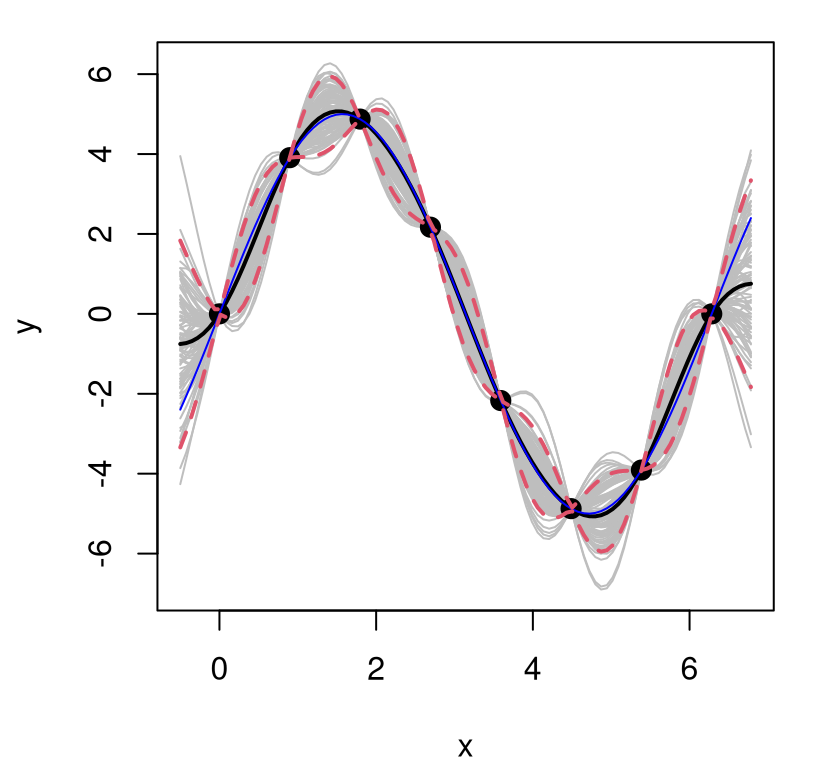
FIGURE 5.9: Sinusoidal GP predictive surface with estimated scale \(\hat{\tau}^2\). Compare to Figure 5.8.
Excepting the appropriately expanded scale of the \(y\)-axis, the view in Figure 5.9 looks nearly identical to Figure 5.3 with data back on the two-unit scale. Besides that this last fit (with \(\hat{\tau}^2\)) looks better (particularly the variance) than the one before it (with implicit \(\tau^2=1\) when the observed scale was really much bigger), how can one be more objective about which is best out-of-sample?
A great paper by Gneiting and Raftery (2007) offers proper scoring rules that facilitate comparisons between predictors in a number of different situations, basically depending on what common distribution characterizes predictors being compared. These are a great resource when comparing apples and oranges, even though we’re about to use them to compare apples to apples: two GPs under different scales.
We have the first two moments, so Eq. (25) from Gneiting and Raftery (2007) may be used. Given \(Y(\mathcal{X})\)-values observed out of sample, the proper scoring rule is given by
\[\begin{equation} \mathrm{score}(Y, \mu, \Sigma; \mathcal{X}) = - \log | \Sigma(\mathcal{X}) | - (Y(\mathcal{X}) - \mu(\mathcal{X}))^\top (\Sigma(\mathcal{X}))^{-1} (Y(\mathcal{X}) - \mu(\mathcal{X})). \tag{5.6} \end{equation}\]
In the case where predictors are actually MVN, which they aren’t quite in our case (they’re Student-\(t\)), this is within an additive constant of what’s called predictive log likelihood. Higher scores, or higher predictive log likelihoods, are better. The first term \(-\log | \Sigma(\mathcal{X})|\) measures magnitude of uncertainty. Smaller uncertainty is better, all things considered, so larger is better here. The second term \((Y(\mathcal{X}) - \mu(\mathcal{X}))^\top (\Sigma(\mathcal{X}))^{-1} (Y(\mathcal{X}) - \mu(\mathcal{X}))\) is mean-squared error (MSE) adjusted for covariance. Smaller MSE is better, but when predictions are inaccurate it’s also important to capture that uncertainty through \(\Sigma(\mathcal{X})\). Score compensates for that second-order consideration: it’s ok to mispredict as long as you know you’re mispredicting.
A more recent paper by Bastos and O’Hagan (2009) tailors the scoring discussion to deterministic computer experiments, which better suits our current setting: interpolating function observations without noise. They recommend using Mahalanobis distance, which for the multivariate Gaussian is the same as the (negative of the) formula above, except without the determinant of \(\Sigma(\mathcal{X})\), and square-rooted.
\[\begin{equation} \mathrm{mah}(y, \mu, \Sigma; \mathcal{X}) = \sqrt{(y(\mathcal{X}) - \mu(\mathcal{X}))^\top (\Sigma(\mathcal{X}))^{-1} (y(\mathcal{X}) - \mu(\mathcal{X}))} \tag{5.7} \end{equation}\]
Smaller distances are otherwise equivalent to higher scores. Here’s code that calculates both in one function.
score <- function(Y, mu, Sigma, mah=FALSE)
 {
  Ymmu <- Y - mu
  Sigmai <- solve(Sigma)
  mahdist <- t(Ymmu) %*% Sigmai %*% Ymmu
  if(mah) return(sqrt(mahdist))
  return (- determinant(Sigma, logarithm=TRUE)$modulus - mahdist)
 }
How about using Mahalanobis distance (Mah for short) to make a comparison between the quality of predictions from our two most recent fits \((\tau^2=1\) versus \(\hat{\tau}^2)\)?
Ytrue <- 5*sin(XX)
df <- data.frame(score(Ytrue, mup, Sigmap, mah=TRUE),
  score(Ytrue, mup2, Sigmap2, mah=TRUE))
colnames(df) <- c("tau2=1", "tau2hat")
df
## tau2=1 tau2hat
## 1 6.259 2.282Estimated scale wins! Actually if you do score without mah=TRUE you come to the opposite conclusion, as Bastos and O’Hagan (2009) caution. Knowledge that the true response is deterministic is important to coming to the correct conclusion about estimates of accuracy as regards variations in scale, in this case, with signal and (lack of) noise contributing to the range of observed measurements. Now what about when there’s noise?
5.2.2 Noise and nuggets
We’ve been saying “regression” for a while, but actually interpolation is a more apt description. Regression is about extracting signal from noise, or about smoothing over noisy data, and so far our example training data have no noise. By inspecting a GP prior, in particular its correlation structure \(C(x, x')\), it’s clear that the current setup precludes idiosyncratic behavior because correlation decays smoothly as a function of distance. Observe that \(C(x,x') \rightarrow 1^-\) as \(x\rightarrow x'\), implying that the closer \(x\) is to \(x'\) the higher the correlation, until correlation is perfect, which is what “connects the dots” when conditioning on data and deriving the predictive distribution.
Moving from GP interpolation to smoothing over noise is all about breaking interpolation, or about breaking continuity in \(C(x,x')\) as \(x\rightarrow x'\). Said another way, we must introduce a discontinuity between diagonal and off-diagonal entries in the correlation matrix \(C_n\) to smooth over noise. There are a lot of ways to skin this cat, and a lot of storytelling that goes with it, but the simplest way to “break it” is with something like
\[ K(x, x') = C(x, x') + g \delta_{x, x'}. \]
Above, \(g > 0\) is a new hyperparameter called the nugget (or sometimes nugget effect), which determines the size of the discontinuity as \(x' \rightarrow x\). The function \(\delta\) is more like the Kronecker delta, although the way it’s written above makes it look like the Dirac delta. Observe that \(g\) generalizes Neal’s \(\epsilon\) jitter.
Neither delta is perfect in terms of describing what to do in practice. The simplest, correct description, of how to break continuity is to only add \(g\) on a diagonal – when indices of \(x\) are the same, not simply for identical values – and nowhere else. Never add \(g\) to an off-diagonal correlation even if that correlation is based on zero distances: i.e., identical \(x\) and \(x'\)-values. Specifically,
- \(K(x_i, x_j) = C(x_i, x_j)\) when \(i \ne j\), even if \(x_i = x_j\);
- only \(K(x_i, x_i) = C(x_i, x_i) + g\).
This leads to the following representation of the data-generating mechanism.
\[ Y \sim \mathcal{N}_n(0, \tau^2 K_n) \]
Unfolding terms, covariance matrix \(\Sigma_n\) contains entries
\[ \Sigma_n^{ij} = \tau^2 (C(x_i, x_j) + g \delta_{ij}), \]
or in other words \(\Sigma_n = \tau^2 K_n = \tau^2(C_n + g \mathbb{I}_n)\). This all looks like a hack, but it’s operationally equivalent to positing the following model.
\[ Y(x) = w(x) + \varepsilon, \]
where \(w(x) \sim \mathcal{GP}\) with scale \(\tau^2\), i.e., \(W \sim \mathcal{N}_n(0, \tau^2 C_n)\), and \(\varepsilon\) is independent Gaussian noise with variance \(\tau^2 g\), i.e., \(\varepsilon \stackrel{\mathrm{iid}}{\sim} \mathcal{N}(0, \tau^2 g)\).
A more aesthetically pleasing model might instead use \(w(x) \sim \mathcal{GP}\) with scale \(\tau^2\), i.e., \(W \sim \mathcal{N}_n(0, \tau^2 C_n)\), and where \(\varepsilon(x)\) is iid Gaussian noise with variance \(\sigma^2\), i.e., \(\varepsilon(x) \stackrel{\mathrm{iid}}{\sim} \mathcal{N}(0, \sigma^2)\). An advantage of this representation is two totally “separate” hyperparameters, with one acting to scale noiseless spatial correlations, and another determining the magnitude of white noise. Those two formulations are actually equivalent. There’s a 1:1 mapping between the two. Many researchers prefer the latter to the former on intuition grounds. But inference in the latter is harder. Conditional on \(g\), \(\hat{\tau}^2\) is available in closed form, which we’ll show momentarily. Conditional on \(\sigma^2\), numerical methods are required for \(\hat{\tau}^2\).
Ok, so back to plan-A with \(Y \sim \mathcal{N}(0, \Sigma_n)\), where \(\Sigma_n = \tau^2 K_n = \tau^2(C_n + g \mathbb{I}_n)\). Recall that \(C_n\) is an \(n \times n\) matrix of inverse exponentiated pairwise squared Euclidean distances. How, then, to estimate two hyperparameters: scale \(\tau^2\) and nugget \(g\)? Again, we have all the usual suspects (MoM, likelihood, CV, variogram) but likelihood-based methods are by far most common. First, suppose that \(g\) is known.
MLE \(\hat{\tau}^2\) given a fixed \(g\) is
\[ \hat{\tau}^2 = \frac{Y_n^\top K_n^{-1} Y_n}{n} = \frac{Y_n^\top (C_n + g \mathbb{I}_n)^{-1} Y_n}{n}. \]
The derivation involves an identical application of Eq. (5.5), except with \(K_n\) instead of \(C_n\).
Plug \(\hat{\tau}^2\) back into our log likelihood to get a concentrated (or profile) log likelihood involving just the remaining parameter \(g\).
\[\begin{align} \ell(g) &= -\frac{n}{2} \log 2\pi - \frac{n}{2} \log \hat{\tau}^2 - \frac{1}{2} \log |K_n| - \frac{1}{2\hat{\tau}^2} Y_n^\top K_n^{-1} Y_n \notag \\ &= c - \frac{n}{2} \log Y_n^\top K_n^{-1} Y_n - \frac{1}{2} \log |K_n| \tag{5.8} \end{align}\]
Unfortunately taking a derivative and setting to zero doesn’t lead to a closed form solution. Calculating the derivative is analytic, which we show below momentarily, but solving is not. Maximizing \(\ell(g)\) requires numerical methods. The simplest thing to do is throw it into optimize and let a polished library do all the work. Since most optimization libraries prefer to minimize, we’ll code up \(-\ell(g)\) in R. The nlg function below doesn’t directly work on X inputs, rather through distances D. This is slightly more efficient since distances can be pre-calculated, rather than re-calculated in each evaluation for new g.
nlg <- function(g, D, Y)
 {
  n <- length(Y)
  K <- exp(-D) + diag(g, n)
  Ki <- solve(K)
  ldetK <- determinant(K, logarithm=TRUE)$modulus
  ll <- - (n/2)*log(t(Y) %*% Ki %*% Y) - (1/2)*ldetK
  counter <<- counter + 1
  return(-ll)
 }
Observe a direct correspondence between nlg and \(-\ell(g)\) with the exception of a counter increment (accessing a global variable). This variable is not required, but we’ll find it handy later when comparing alternatives on efficiency grounds in numerical optimization, via the number of times our likelihood objective function is evaluated. Although optimization libraries often provide iteration counts on output, sometimes that report can misrepresent the actual number of objective function calls. So I’ve jerry-rigged my own counter here to fill in.
Example: noisy 1d sinusoid
Before illustrating numerical nugget (and scale) optimization towards the MLE, we need some example data. Let’s return to our running sinusoid example from §5.1.1, picking up where we left off but augmented with standard Gaussian noise. Code below utilizes the same uniform Xs from earlier, but doubles them up. Adding replication into a design is recommended in noisy data contexts, as discussed in more detail in Chapter 10. Replication is not essential for this example, but it helps guarantee predictable outcomes which is important for a randomly seeded, fully reproducible Rmarkdown build.
Everything is in place to estimate the optimal nugget. The optimize function in R is ideal in 1d derivative-free contexts. It doesn’t require an initial value for g, but it does demand a search interval. A sensible yet conservative range for \(g\)-values is from eps to var(y). The former corresponds to the noise-free/jitter-only case we entertained earlier. The latter is the observed marginal variance of \(Y\), or in other words about as big as variance could be if these data were all noise and no signal.
## [1] 0.2878Now the value of that estimate isn’t directly useful to us, at least on an intuitive level. We need \(\hat{\tau}^2\) to understand the full decomposition of variance. But backing out those quantities is relatively straightforward.
K <- exp(-D) + diag(g, n)
Ki <- solve(K)
tau2hat <- drop(t(y) %*% Ki %*% y / n)
c(tau=sqrt(tau2hat), sigma=sqrt(tau2hat*g))
## tau sigma
## 2.304 1.236Both are close to their true values of \(5/2 = 2.5\) and 1, respectively. Estimated hyperparameters in hand, prediction is a straightforward application of MVN conditionals. First calculate quantities involved in covariance between testing and training locations, and between testing locations and themselves.
Notice that only KXX is augmented with g on the diagonal. KX is not a square symmetric matrix calculated from identically indexed \(x\)-values. Even if it were coincidentally square, or if DX contained zero distances because elements of XX and X coincide, still no nugget augmentation is deployed. Only with KXX, which is identically indexed with respect to itself, does a nugget augment the diagonal.
Covariance matrices in hand, we may then calculate the predictive mean vector and covariance matrix.
mup <- KX %*% Ki %*% y
Sigmap <- tau2hat*(KXX - KX %*% Ki %*% t(KX))
q1 <- mup + qnorm(0.05, 0, sqrt(diag(Sigmap)))
q2 <- mup + qnorm(0.95, 0, sqrt(diag(Sigmap)))
Showing sample predictive realizations that look pretty requires “subtracting” out idiosyncratic noise, i.e., the part due to nugget \(g\). Otherwise sample paths will be “jagged” and hard to interpret.
Sigma.int <- tau2hat*(exp(-DXX) + diag(eps, nrow(DXX))
  - KX %*% Ki %*% t(KX))
YY <- rmvnorm(100, mup, Sigma.int)§5.3.2 explains how this maneuver makes sense in a latent function-space view of GP posterior updating, and again when we delve into a deeper signal-to-noise discussion in Chapter 10. For now this is just a trick to get a prettier picture, only affecting gray lines plotted in Figure 5.10.
matplot(XX, t(YY), type="l", lty=1, col="gray", xlab="x", ylab="y")
points(X, y, pch=20, cex=2)
lines(XX, mup, lwd=2)
lines(XX, 5*sin(XX), col="blue")
lines(XX, q1, lwd=2, lty=2, col=2)
lines(XX, q2, lwd=2, lty=2, col=2)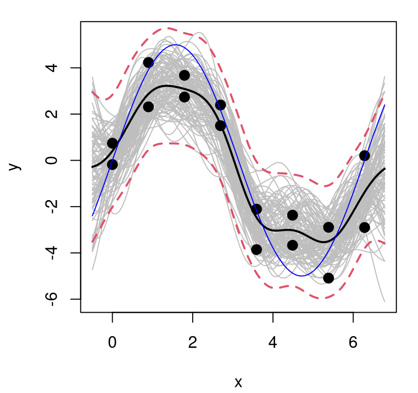
FIGURE 5.10: GP fit to sinusoidal data with estimated nugget.
Notice how the error-bars, which do provide a full accounting of predictive uncertainty, lie mostly outside of the gray lines and appropriately capture variability in the training data observations, shown as filled black dots. That’s it: now we can fit noisy data with GPs using a simple library-based numerical optimizer and about twenty lines of code.
5.2.3 Derivative-based hyperparameter optimization
It can be unsatisfying to brute-force an optimization for a hyperparameter like \(g\), even though 1d solving with optimize is often superior to cleverer methods. Can we improve upon the number of evaluations?
## [1] 16Actually, that’s pretty good. If you can already optimize numerically in fewer than twenty or so evaluations there isn’t much scope for improvement. Yet we’re leaving information on the table: closed-form derivatives. Differentiating \(\ell(g)\) involves pushing the chain rule through the inverse of covariance matrix \(K_n\) and its determinant, which is where hyperparameter \(g\) is involved. The following identities, which are framed for an arbitrary parameter \(\phi\), will come in handy.
\[\begin{equation} \frac{\partial K_n^{-1}}{\partial \phi} = - K_n^{-1} \frac{\partial K_n}{\partial \phi} K_n^{-1} \quad \mbox{ and } \quad \frac{\partial \log | K_n | }{\partial \phi} = \mathrm{tr} \left \{ K_n^{-1} \frac{\partial K_n}{\partial \phi} \right\} \tag{5.9} \end{equation}\]
The chain rule, and a single application of each of the identities above, gives
\[\begin{align} \ell'(g) &= - \frac{n}{2} \frac{Y_n^\top \frac{\partial K_n^{-1}}{\partial g} Y_n}{Y_n^\top K_n^{-1} Y_n} - \frac{1}{2} \frac{\partial \log |K_n|}{\partial g} \tag{5.10} \\ &= \frac{n}{2} \frac{Y_n^\top K_n^{-1} \frac{\partial K_n}{\partial g} K_n^{-1} Y_n}{Y_n^\top K_n^{-1} Y_n} - \frac{1}{2} \mathrm{tr} \left \{ K_n^{-1} \frac{\partial K_n}{\partial g} \right\}. \notag \end{align}\]
Off-diagonal elements of \(K_n\) don’t depend on \(g\). The diagonal is simply \(1 + g\). Therefore \(\frac{\partial K_n}{\partial g}\) is an \(n\)-dimensional identity matrix. Putting it all together:
\[ \ell'(g) = \frac{n}{2} \frac{Y_n^\top (K_n^{-1})^{2} Y_n}{Y_n^\top K_n^{-1} Y_n} - \frac{1}{2} \mathrm{tr} \left \{ K_n^{-1} \right\}. \]
Here’s an implementation of the negative of that derivative for the purpose of minimization. The letter “g” for gradient in the function name is overkill in this scalar context, but I’m thinking ahead to where yet more hyperparameters will be optimized.
gnlg <- function(g, D, Y)
 {
  n <- length(Y)
  K <- exp(-D) + diag(g, n)
  Ki <- solve(K)
  KiY <- Ki %*% Y
  dll <- (n/2) * t(KiY) %*% KiY / (t(Y) %*% KiY) - (1/2)*sum(diag(Ki))
  return(-dll)
 }
Objective (negative concentrated log likelihood, nlg) and gradient (gnlg) in hand, we’re ready to numerically optimize using derivative information. The optimize function doesn’t support derivatives, so we’ll use optim instead. The optim function supports many optimization methods, and not all accommodate derivatives. I’ve chosen to illustrate method="L-BFGS-B" here because it supports derivatives and allows bound constraints (Byrd et al. 1995). As above, we know we don’t want a nugget lower than eps for numerical reasons, and it seems unlikely that \(g\) will be bigger than the marginal variance.
Here we go … first reinitializing the evaluation counter and choosing 10% of marginal variance as a starting value.
counter <- 0
out <- optim(0.1*var(y), nlg, gnlg, method="L-BFGS-B", lower=eps,
  upper=var(y), D=D, Y=y)
c(g, out$par)
## [1] 0.2878 0.2879Output is similar to what we obtained from optimize, which is reassuring. How many iterations?
## function gradient   actual
##        8        8        8
Notice that in this scalar case our internal, manual counter agrees with optim’s. Just 8 evaluations to optimize something is pretty excellent,
but possibly not noteworthy compared to optimize’s 16, especially when you consider that an extra 8 gradient evaluations (with similar computational complexity) are also required. When you put it that way, our new derivative-based version is potentially no better, requiring 16 combined evaluations of commensurate computational complexity. Hold that thought. We shall return to counting iterations after introducing more hyperparameters.
5.2.4 Lengthscale: rate of decay of correlation
How about modulating the rate of decay of spatial correlation in terms of distance? Surely unadulterated Euclidean distance isn’t equally suited to all data. Consider the following generalization, known as the isotropic Gaussian family.
\[ C_\theta(x, x') = \exp\left\{ - \frac{||x - x'||^2}{\theta} \right\} \]
Isotropic Gaussian correlation functions are indexed by a scalar hyperparameter \(\theta\), called the characteristic lengthscale. Sometimes this is shortened to lengthscale, or \(\theta\) may be referred to as a range parameter, especially in geostatistics. When \(\theta = 1\) we get back our inverse exponentiated squared Euclidean distance-based correlation as a special case. Isotropy means that correlation decays radially; Gaussian suggests inverse exponentiated squared Euclidean distance. Gaussian processes should not be confused with Gaussian-family correlation or kernel functions, which appear in many contexts. GPs get their name from their connection with the MVN, not because they often feature Gaussian kernels as a component of the covariance structure. Further discussion of kernel variations and properties is deferred until later in §5.3.3.
How to perform inference for \(\theta\)? Should our GP have a slow decay of correlation in space, leading to visually smooth/slowly changing surfaces, or a fast one looking more wiggly? Like with nugget \(g\), embedding \(\theta\) deep within coordinates of a covariance matrix thwarts analytic maximization of log likelihood. Yet again like \(g\), numerical methods are rather straightforward. In fact the setup is identical except now we have two unknown hyperparameters.
Consider brute-force optimization without derivatives. The R function nl is identical to nlg except argument par takes in a two-vector whose first coordinate is \(\theta\) and second is \(g\). Only two lines differ, and those are indicated by comments in the code below.
nl <- function(par, D, Y)
 {
  theta <- par[1]                                       ## change 1
  g <- par[2]
  n <- length(Y)
  K <- exp(-D/theta) + diag(g, n)                       ## change 2
  Ki <- solve(K)
  ldetK <- determinant(K, logarithm=TRUE)$modulus
  ll <- - (n/2)*log(t(Y) %*% Ki %*% Y) - (1/2)*ldetK
  counter <<- counter + 1
  return(-ll)
 }
That’s it: just shove it into optim. Note that optimize isn’t an option here as that routine only optimizes in 1d. But first we’ll need an example. For variety, consider again our 2d exponential data from §5.1.2 and Figure 5.5, this time observed with noise and entertaining non-unit lengthscales.
library(lhs)
X2 <- randomLHS(40, 2)
X2 <- rbind(X2, X2)
X2[,1] <- (X2[,1] - 0.5)*6 + 1
X2[,2] <- (X2[,2] - 0.5)*6 + 1
y2 <- X2[,1]*exp(-X2[,1]^2 - X2[,2]^2) + rnorm(nrow(X2), sd=0.01)
Again, replication is helpful for stability in reproduction, but is not absolutely necessary. Estimating lengthscale and nugget simultaneously represents an attempt to strike balance between signal and noise (Chapter 10). Once we get more experience, we’ll see that long lengthscales are more common when noise/nugget is high, whereas short lengthscales offer the potential to explain away noise as quickly changing dynamics in the data. Sometimes choosing between those two can be a difficult enterprise.
With optim it helps to think a little about starting values and search ranges. The nugget is rather straightforward, and we’ll copy ranges and starting values from our earlier example: from \(\epsilon\) to \(\mathbb{V}\mathrm{ar}\{Y\}\). The lengthscale is a little harder. Sensible choices for \(\theta\) follow the following rationale, leveraging \(x\)-values in coded units (\(\in [0,1]^2\)). A lengthscale of 0.1, which is about \(\sqrt{0.1} = 0.32\) in units of \(x\), biases towards surfaces three times more wiggly than in our earlier setup, with implicit \(\theta = 1\), in a certain loose sense. More precise assessments are quoted later after learning more about kernel properties (§5.3.3) and upcrossings (5.17). Initializing in a more signal, less noise regime seems prudent. If we thought the response was “really straight”, perhaps an ordinary linear model would suffice. A lower bound of eps allows the optimizer to find even wigglier surfaces, however it might be sensible to view solutions close to eps as suspect. A value of \(\theta=10\), or \(\sqrt{10} = 3.16\) is commensurately (3x) less wiggly than our earlier analysis. If we find a \(\hat{\theta}\) on this upper boundary we can always re-run with a new, bigger upper bound. For a more in-depth discussion of suitable lengthscale and nugget ranges, and even priors for regularization, see Appendix A of the tutorial (Gramacy 2016) for the laGP library (Gramacy and Sun 2018) introduced in more detail in §5.2.6.
Ok, here we go. (With new X we must first refresh D.)
D <- distance(X2)
counter <- 0
out <- optim(c(0.1, 0.1*var(y2)), nl, method="L-BFGS-B", lower=eps,
  upper=c(10, var(y2)), D=D, Y=y2)
out$par
## [1] 0.920257 0.009167Actually the outcome, as regards the first coordinate \(\hat{\theta}\), is pretty close to our initial version with implied \(\theta = 1\). Since "L-BFGS-B" is calculating a gradient numerically through finite differences, the reported count of evaluations in the output doesn’t match the number of actual evaluations.
## function gradient   actual
##       13       13       65
We’re searching in two input dimensions, and a rule of thumb is that it takes two evaluations in each dimension to build a tangent plane to approximate a derivative. So if 13 function evaluations are reported, it’d take about \(2\times 2 \rightarrow 4 \times 13 = 52\) additional runs to approximate derivatives, which agrees with our “by-hand” counter.
How can we improve upon those counts? Reducing the number of evaluations should speed up computation time. It might not be a big deal now, but as \(n\) gets bigger the repeated cubic cost of matrix inverses and determinants really adds up. What if we take derivatives with respect to \(\theta\) and combine with those for \(g\) to form a gradient? That requires \(\dot{K}_n \equiv \frac{\partial K_n}{\partial \theta}\), to plug into inverse and determinant derivative identities (5.9). The diagonal is zero because the exponent is zero no matter what \(\theta\) is. Off-diagonal entries of \(\dot{K}_n\) work out as follows. Since
\[ \begin{aligned} K_\theta(x, x') &= \exp\left\{ - \frac{||x - x'||^2}{\theta} \right\}, & \mbox{we have} && \frac{\partial K_\theta(x_i, x_j)}{\partial \theta} &= K_\theta(x_i, x_j) \frac{||x_i - x_j||^2}{\theta^2}. \\ \end{aligned} \]
A slightly more compact way to write the same thing would be \(\dot{K}_n = K_n \circ \mathrm{Dist}_n/\theta^2\) where \(\circ\) is a component-wise, Hadamard product, and \(\mathrm{Dist}_n\) contains a matrix of squared Euclidean distances – our D in the code. An identical application of the chain rule for the nugget (5.10), but this time for \(\theta\), gives
\[\begin{equation} \ell'(\theta) \equiv \frac{\partial}{\partial \theta} \ell(\theta, g) = \frac{n}{2} \frac{Y_n^\top K_n^{-1} \dot{K}_n K_n^{-1} Y_n}{Y_n^\top K_n^{-1} Y_n} - \frac{1}{2} \mathrm{tr} \left \{ K_n^{-1} \dot{K}_n \right\}. \tag{5.11} \end{equation}\]
A vector collecting the two sets of derivatives forms the gradient of \(\ell(\theta, g)\), a joint log likelihood with \(\tau^2\) concentrated out. R code below implements the negative of that gradient for the purposes of MLE calculation with optim minimization. Comments therein help explain the steps involved.
gradnl <- function(par, D, Y)
 {
  ## extract parameters
  theta <- par[1]
  g <- par[2]

  ## calculate covariance quantities from data and parameters
  n <- length(Y)
  K <- exp(-D/theta) + diag(g, n)
  Ki <- solve(K)
  dotK <- K*D/theta^2
  KiY <- Ki %*% Y

  ## theta component
  dlltheta <- (n/2) * t(KiY) %*% dotK %*% KiY / (t(Y) %*% KiY) -
    (1/2)*sum(diag(Ki %*% dotK))

  ## g component
  dllg <- (n/2) * t(KiY) %*% KiY / (t(Y) %*% KiY) - (1/2)*sum(diag(Ki))

  ## combine the components into a gradient vector
  return(-c(dlltheta, dllg))
 }
How well does optim work when it has access to actual gradient evaluations? Observe here that we’re otherwise using exactly the same calls as earlier.
counter <- 0
outg <- optim(c(0.1, 0.1*var(y2)), nl, gradnl, method="L-BFGS-B",
  lower=eps, upper=c(10, var(y2)), D=D, Y=y2)
rbind(grad=outg$par, brute=out$par)
## [,1] [,2]
## grad 0.9203 0.009167
## brute 0.9203 0.009167Parameter estimates are nearly identical. Availability of a true gradient evaluation changes the steps of the algorithm slightly, often leading to a different end-result even when identical convergence criteria are applied. What about the number of evaluations?
##       function gradient actual
## grad        10       10     10
## brute       13       13     65
Woah! That’s way better. No only does our actual “by-hand” count of evaluations match what’s reported on output from optim, but it can be an order of magnitude lower, roughly, compared to what we had before. (Variations depend on the random data used to generate this Rmarkdown document.) A factor of five-to-ten savings is definitely worth the extra effort to derive and code up a gradient. As you can imagine, and we’ll show shortly, gradients are commensurately more valuable when there are even more hyperparameters. “But what other hyperparameters?”, you ask. Hold that thought.
Optimized hyperparameters in hand, we can go about rebuilding quantities required for prediction. Begin with training quantities …
K <- exp(- D/outg$par[1]) + diag(outg$par[2], nrow(X2))
Ki <- solve(K)
tau2hat <- drop(t(y2) %*% Ki %*% y2 / nrow(X2))
… then predictive/testing ones …
gn <- 40
xx <- seq(-2, 4, length=gn)
XX <- expand.grid(xx, xx)
DXX <- distance(XX)
KXX <- exp(-DXX/outg$par[1]) + diag(outg$par[2], ncol(DXX))
DX <- distance(XX, X2)
KX <- exp(-DX/outg$par[1])
… and finally kriging equations.
The resulting predictive surfaces look pretty much the same as before, as shown in Figure 5.11.
par(mfrow=c(1,2))
image(xx, xx, matrix(mup, ncol=gn), main="mean", xlab="x1",
  ylab="x2", col=cols)
points(X2)
image(xx, xx, matrix(sdp, ncol=gn), main="sd", xlab="x1",
  ylab="x2", col=cols)
points(X2)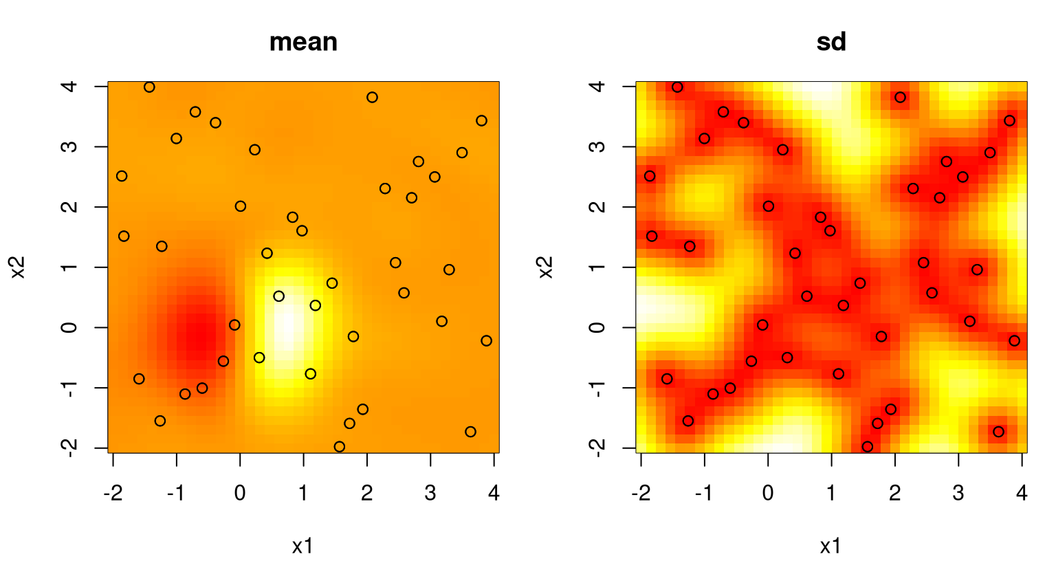
FIGURE 5.11: Predictive mean (left) and standard deviation (right) after estimating a lengthscale \(\hat{\theta}\).
This is perhaps not an exciting way to end the example, but it serves to illustrate the basic idea of estimating unknown quantities and plugging them into predictive equations. I’ve only illustrated 1d and 2d so far, but the principle is no different in higher dimensions.
5.2.5 Anisotropic modeling
It’s time to expand input dimension a bit, and get ambitious. Visualization will be challenging, but there are other metrics of success. Consider the Friedman function, a popular toy problem from the seminal multivariate adaptive regression splines [MARS; Friedman (1991)] paper. Splines are a popular alternative to GPs in low input dimension. The idea is to “stitch” together low-order polynomials. The “stitching boundary” becomes exponentially huge as dimension increases, which challenges computation. For more details, see the splines supplement linked here which is based on Hastie, Tibshirani, and Friedman (2009), Chapters 5, 7 and 8. MARS circumvents many of those computational challenges by simplifying basis elements (to piecewise linear) on main effects and limiting (to two-way) interactions. Over-fitting is mitigated by aggressively pruning useless basis elements with a generalized CV scheme.
fried <- function(n=50, m=6)
 {
  if(m < 5) stop("must have at least 5 cols")
  X <- randomLHS(n, m)
  Ytrue <- 10*sin(pi*X[,1]*X[,2]) + 20*(X[,3] - 0.5)^2 + 10*X[,4] + 5*X[,5]
  Y <- Ytrue + rnorm(n, 0, 1)
  return(data.frame(X, Y, Ytrue))
 }
The surface is nonlinear in five input coordinates,
\[\begin{equation} \mathbb{E}\{Y(x)\} = 10 \sin(\pi x_1 x_2) + 20(x_3 - 0.5)^2 + 10x_4 - 5x_5, \tag{5.12} \end{equation}\]
combining periodic, quadratic and linear effects. Notice that you can ask for more (useless) coordinates if you want: inputs \(x_6, x_7, \dots\) The fried function, as written above, generates both the \(X\)-values, via LHS (§4.1) in \([0,1]^m\), and \(Y\)-values. Let’s create training and testing sets in seven input dimensions, i.e., with two irrelevant inputs \(x_6\) and \(x_7\). Code below uses fried to generate an LHS training–testing partition (see, e.g., Figure 4.9) with \(n=200\) and \(n' = 1000\) observations, respectively. Such a partition could represent one instance in the “bakeoff” described by Algorithm 4.1. See §5.2.7 for iteration on that theme.
m <- 7
n <- 200
nprime <- 1000
data <- fried(n + nprime, m)
X <- as.matrix(data[1:n,1:m])
y <- drop(data$Y[1:n])
XX <- as.matrix(data[(n + 1):(n + nprime),1:m])
yy <- drop(data$Y[(n + 1):(n + nprime)])
yytrue <- drop(data$Ytrue[(n + 1):(n + nprime)])
The code above extracts two types of \(Y\)-values for use in out-of-sample testing. De-noised yytrue values facilitate comparison with root mean-squared error (RMSE),
\[\begin{equation} \sqrt{\frac{1}{n'} \sum_{i=1}^{n'} (y_i - \mu(x_i))^2}. \tag{5.13} \end{equation}\]
Notice that RMSE is square-root Mahalanobis distance (5.7) calculated with an identity covariance matrix. Noisy out-of-sample evaluations yy can be used for comparison by proper score (5.6), combining both mean accuracy and estimates of covariance.
First learning. Inputs X and outputs y are re-defined, overwriting those from earlier examples. After re-calculating pairwise distances D, we may cut-and-paste gradient-based optim on objective nl and gradient gnl.
D <- distance(X)
out <- optim(c(0.1, 0.1*var(y)), nl, gradnl, method="L-BFGS-B", lower=eps,
  upper=c(10, var(y)), D=D, Y=y)
out
## $par
## [1] 2.533216 0.005201
##
## $value
## [1] 683.5
##
## $counts
## function gradient
## 33 33
##
## $convergence
## [1] 0
##
## $message
## [1] "CONVERGENCE: REL_REDUCTION_OF_F <= FACTR*EPSMCH"Output indicates convergence has been achieved. Based on estimated \(\hat{\theta} = 2.533\) and \(\hat{g} = 0.0052\), we may rebuild the data covariance quantities …
K <- exp(- D/out$par[1]) + diag(out$par[2], nrow(D))
Ki <- solve(K)
tau2hat <- drop(t(y) %*% Ki %*% y / nrow(D))
… as well as those involved in predicting at XX testing locations.
DXX <- distance(XX)
KXX <- exp(-DXX/out$par[1]) + diag(out$par[2], ncol(DXX))
DX <- distance(XX, X)
KX <- exp(-DX/out$par[1])
Kriging equations are then derived as follows.
Notice how not a single line in the code above, pasted directly from identical lines used in earlier examples, requires tweaking to accommodate the novel 7d setting. Our previous examples were in 1d and 2d, but the code works verbatim in 7d. However the number of evaluations required to maximize is greater now than in previous examples. Here we have 33 compared to 10 previously in 2d.
How accurate are predictions? RMSE on the testing set is calculated below, but we don’t yet have a benchmark to compare this to.
## gpiso
## 1.107How about comparing to MARS? That seems natural considering these data were created as a showcase for that very method. MARS implementations can be found in the mda (Leisch, Hornik, and Ripley 2017) and earth (Milborrow 2019) packages on CRAN.
Which wins between the isotropic GP and MARS based on RMSE to the truth?
## gpiso mars
## 1.107 1.518Usually the GP wins in this comparison. In about one time out of twenty random Rmarkdown rebuilds MARS wins. Unfortunately MARS doesn’t natively provide a notion of predictive variance. That is, not without an extra bootstrap layer or a Bayesian treatment; e.g., see BASS (Francom 2017) on CRAN. So a comparison to MARS by proper score isn’t readily available. Some may argue that this comparison isn’t fair. MARS software has lots of tuning parameters that we aren’t exploring. Results from mars improve with argument degree=2 and, for reasons that aren’t immediately clear to me at this time, they’re even better with earth after the same degree=2 modification. I’ve deliberately put up a relatively “vanilla” straw man in this comparison. This is in part because our GP setup is itself relatively vanilla. An exercise in §5.5 invites the reader to explore a wider range of alternatives on both fronts.
How can we add more flavor? If that was vanilla GP regression, what does rocky road look like? To help motivate, recall that the Friedman function involved a diverse combination of effects on the input variables: trigonometric, quadratic and linear. Although we wouldn’t generally know that much detail in a new application – and GPs excel in settings where little is known about input–output relationships, except perhaps that it might be worth trying methods beyond the familiar linear model – it’s worth wondering if our modeling apparatus is not at odds with typically encountered dynamics. More to the point, GP modeling flexibility comes from the MVN covariance structure which is based on scaled (by \(\theta\)) inverse exponentiated squared Euclidean distance. That structure implies uniform decay in correlation in each input direction. Is such radial symmetry reasonable? Probably not in general, and definitely not in the case of the Friedman function.
How about the following generalization?
\[ C_\theta(x, x') = \exp\left\{ - \sum_{k=1}^m \frac{(x_k - x'_k)^2}{\theta_k} \right\} \]
Here we’re using a vectorized lengthscale parameter \(\theta = (\theta_1,\dots,\theta_m)\), allowing strength of correlation to be modulated separately by distance in each input coordinate. This family of correlation functions is called the separable or anisotropic Gaussian. Separable because the sum is a product when taken outside the exponent, implying independence in each coordinate direction. Anisotopic because, except in the special case where all \(\theta_k\) are equal, decay of correlation is not radial.
How does one perform inference for such a vectorized parameter? Simple; just expand log likelihood and derivative functions to work with vectorized \(\theta\). Thinking about implementation: a for loop in the gradient function can iterate over coordinates, wherein each iteration we plug
\[\begin{equation} \frac{\partial K_n^{ij}}{\partial \theta_k} = K_n^{ij} \frac{(x_{ik} - x_{jk})^2}{\theta_k^2} \tag{5.14} \end{equation}\]
into our formula for \(\ell'(\theta_k)\) in Eq. (5.11), which is otherwise unchanged.
Each coordinate has a different \(\theta_k\), so pre-computing a distance matrix isn’t helpful. Instead we’ll use the covar.sep function from the plgp package which takes vectorized d \(\equiv \theta\) and scalar g arguments, combing distance and inverse-scaling into one step. Rather than going derivative crazy immediately, let’s focus on the likelihood first, which we’ll need anyways before going “whole hog”. The function below is nearly identical to nl from §5.2.4 except the first ncol(X) components of argument par are sectioned off for theta, and covar.sep is used directly on X inputs rather than operating on pre-calculated D.
nlsep <- function(par, X, Y)
{
theta <- par[1:ncol(X)]
g <- par[ncol(X)+1]
n <- length(Y)
K <- covar.sep(X, d=theta, g=g)
Ki <- solve(K)
ldetK <- determinant(K, logarithm=TRUE)$modulus
ll <- - (n/2)*log(t(Y) %*% Ki %*% Y) - (1/2)*ldetK
counter <<- counter + 1
return(-ll)
}As a testament to how easy it is to optimize that likelihood, at least in terms of coding, below we port our optim on nl above to nlsep below with the only change being to repeat upper and lower arguments, and supply X instead of D. (Extra commands for timing will be discussed momentarily.)
tic <- proc.time()[3]
counter <- 0
out <- optim(c(rep(0.1, ncol(X)), 0.1*var(y)), nlsep, method="L-BFGS-B",
X=X, Y=y, lower=eps, upper=c(rep(10, ncol(X)), var(y)))
toc <- proc.time()[3]
out$par## [1] 1.120385 1.075619 1.775699 9.047709 10.000000 10.000000
## [7] 9.256984 0.008255What can be seen on output? Notice how \(\hat{\theta}_k\)-values track what we know about the Friedman function. The first three inputs have relatively shorter lengthscales compared to inputs four and five. Recall that shorter lengthscale means “more wiggly”, which is appropriate for those nonlinear terms; longer lengthscale corresponds to linearly contributing inputs. Finally, the last two (save \(g\) in the final position of out$par) also have long lengthscales, which is similarly reasonable for inputs which aren’t contributing.
But how about the number of evaluations?
## function gradient actual
## 66 66 1122Woah, lots! Although only 66 optimization steps were required, in 8d (including nugget g in par) that amounts to evaluating the objective function more than one-thousand-odd times, plus-or-minus depending on the random Rmarkdown build. When \(n = 200\), and with cubic matrix decompositions, that can be quite a slog time-wise: about 9 seconds.
## elapsed
## 8.716To attempt to improve on that slow state of affairs, code below implements a gradient (5.14) for vectorized \(\theta\).
gradnlsep <- function(par, X, Y)
{
theta <- par[1:ncol(X)]
g <- par[ncol(X)+1]
n <- length(Y)
K <- covar.sep(X, d=theta, g=g)
Ki <- solve(K)
KiY <- Ki %*% Y
## loop over theta components
dlltheta <- rep(NA, length(theta))
for(k in 1:length(dlltheta)) {
dotK <- K * distance(X[,k])/(theta[k]^2)
dlltheta[k] <- (n/2) * t(KiY) %*% dotK %*% KiY / (t(Y) %*% KiY) -
(1/2)*sum(diag(Ki %*% dotK))
}
## for g
dllg <- (n/2) * t(KiY) %*% KiY / (t(Y) %*% KiY) - (1/2)*sum(diag(Ki))
return(-c(dlltheta, dllg))
}Here’s what you get when you feed gradnlsep into optim, otherwise with the same calls as before.
tic <- proc.time()[3]
counter <- 0
outg <- optim(c(rep(0.1, ncol(X)), 0.1*var(y)), nlsep, gradnlsep,
method="L-BFGS-B", lower=eps, upper=c(rep(10, ncol(X)), var(y)), X=X, Y=y)
toc <- proc.time()[3]
thetahat <- rbind(grad=outg$par, brute=out$par)
colnames(thetahat) <- c(paste0("d", 1:ncol(X)), "g")
thetahat## d1 d2 d3 d4 d5 d6 d7 g
## grad 1.115 1.004 1.678 7.412 10 10 8.851 0.008911
## brute 1.120 1.076 1.776 9.048 10 10 9.257 0.008255First, observe the similar, but not always identical result in terms of optimized parameter(s). Derivatives enhance accuracy and alter convergence criteria compared to tangent-based approximations which sometimes leads to small discrepancies. How about number of evaluations?
## function gradient actual
## grad 135 135 135
## brute 66 66 1122Far fewer; an order of magnitude fewer actually, and that pays dividends in time.
## elapsed
## 5.782Unfortunately, it’s not \(10\times\) faster with \(10\times\) fewer evaluations because gradient evaluation takes time. Evaluating each derivative component – each iteration of the for loop in gradnlsep – involves a matrix multiplication quadratic in \(n\). So that’s eight more quadratic-\(n\)-cost operations per evaluation compared to one for nlsep alone. Consequently, we see a 2–3\(\times\) speedup. There are some inefficiencies in this implementation. For example, notice that nlsep and gradnlsep repeat some calculations. Also the matrix trace implementation, sum(diag(Ki %*% dotK) is wasteful. Yet again I’ll ask you to hold that thought for when we get to library-based implementations, momentarily.
Ok, we got onto this tangent after wondering if GPs could do much better, in terms of prediction, on the Friedman data. So how does a separable GP compare against the isotropic one and MARS? First, take MLE hyperparameters and plug them into the predictive equations.
K <- covar.sep(X, d=outg$par[1:ncol(X)], g=outg$par[ncol(X)+1])
Ki <- solve(K)
tau2hat <- drop(t(y) %*% Ki %*% y / nrow(X))
KXX <- covar.sep(XX, d=outg$par[1:ncol(X)], g=outg$par[ncol(X)+1])
KX <- covar.sep(XX, X, d=outg$par[1:ncol(X)], g=0)
mup2 <- KX %*% Ki %*% y
Sigmap2 <- tau2hat*(KXX - KX %*% Ki %*% t(KX))A 2 is tacked onto the variable names above so as not to trample on isotropic analogs. We’ll need both sets of variables to make a comparison based on score shortly. But first, here are RMSEs.
## gpiso mars gpsep
## 1.1071 1.5176 0.6512The separable covariance structure performs much better. Whereas the isotropic GP only beats MARS 19/20 times in random Rmarkdown builds, the separable GP is never worse than MARS, and it’s also never worse than its isotropic cousin. It pays to learn separate lengthscales for each input coordinate.
Since GPs emit full covariance structures we can also make a comparison by proper score (5.6). Mahalanobis distance is not appropriate here because training responses are not deterministic. Score calculations should commence on yy here, i.e., with noise, not on yytrue which is deterministic.
## gp mars gpsep
## -1346 NA -1162Recall that larger scores are better; so again the separable GP wins.
5.2.6 Library
All this cutting-and-pasting is getting a bit repetitive. Isn’t there a library for that? Yes, several! But first, this might be a good opportunity to pin down the steps for GP regression in a formal boxed algorithm. Think of it as a capstone. Some steps in Algorithm 5.1 are a little informal since the equations are long, and provided earlier. There are many variations/choices on exactly how to proceed, especially to do with MVN correlation structure, or kernel. More options follow, i.e., beyond isotropic and separable Gaussian variations, later in the chapter.
Algorithm 5.1: Gaussian Process Regression
Assume correlation structure \(K(\cdot, \cdot)\) has been chosen, which may include hyperparameter lengthscale (vector) \(\theta\) and nugget \(g\); we simply refer to a combined \(\theta \equiv (\theta, g)\) below.
Require \(n \times m\) matrix of inputs \(X_n\) and \(n\)-vector of outputs \(Y_n\); optionally an \(n' \times m\) matrix of predictive locations \(\mathcal{X}\).
Then
- Derive the concentrated log likelihood \(\ell(\theta)\) following Eq. (5.8) under MVN sampling model with hyperparameters \(\theta\) and develop code to evaluate that likelihood as a function of \(\theta\).
- Variations may depend on choice of \(K(\cdot, \cdot)\), otherwise the referenced equations can be applied directly.
- Optionally, differentiate that log likelihood (5.11) with respect to \(\theta\), forming a gradient \(\ell'(\theta) \equiv \nabla \ell(\theta)\), and implement it too as a code which can be evaluated as a function of \(\theta\).
- Referenced equations apply directly so long as \(\dot{K}_n\), the derivative of the covariance matrix with respect to the components of \(\theta\), may be evaluated.
- Choose initial values and search ranges for the components of \(\theta\) being optimized.
- Plug log likelihood and (optionally) gradient code into your favorite optimizer (e.g.,
optimwithmethod="L-BFGS-B"), along with initial values and ranges, obtaining \(\hat{\theta}\).- If any components of \(\hat{\theta}\) are on the boundary of the chosen search range, consider expanding those ranges and repeat step 3.
- If \(\mathcal{X}\) is provided, plug \(\hat{\theta}\) and \(\mathcal{X}\) into either pointwise (5.2) or joint (5.3) predictive equations.
Return MLE \(\hat{\theta}\), which can be used later for predictions; mean vector \(\mu(\mathcal{X})\) and covariance matrix \(\Sigma(\mathcal{X})\) or variance vector \(\sigma^2(\mathcal{X})\) if \(\mathcal{X}\) provided.
Referenced equations in the algorithm are meant as examples. Text surrounding those links offers more context about how such equations are intended to be applied. Observe that the description treats predictive/testing locations \(\mathcal{X}\) as optional. It’s quite common in implementation to separate inference and prediction, however Algorithm 5.1 combines them. If new \(\mathcal{X}\) comes along, steps 1–4 can be skipped if \(\hat{\theta}\) has been saved. If \(\hat{\tau}^2\) and \(K_n^{-1}\), which depend on \(\hat{\theta}\), have also been saved then pointwise prediction is quadratic in \(n\). They’re quadratic in \(n'\) when a full predictive covariance \(\Sigma(\mathcal{X})\) is desired, which may be problematic for large grids. Evaluating those equations, say to obtain draws, necessitates decomposition and is thus cubic in \(n'\).
There are many libraries automating the process outlined by Algorithm 5.1, providing several choices of families of covariance functions and variations in hyperparameterization. For R these include mlegp (Dancik 2018), GPfit (MacDonald, Chipman, and Ranjan 2019), spatial (Ripley 2015) fields (Nychka et al. 2019), RobustGaSP (Gu, Palomo, and Berger 2018), and kernlab (Karatzoglou, Smola, and Hornik 2018) – all performing maximum likelihood (or maximum a posteriori/Bayesian regularized) point inference; or tgp (Gramacy and Taddy 2016), emulator (Hankin 2019), plgp, and spBayes (A. Finley and Banerjee 2019) – performing fully Bayesian inference. There are a few more that will be of greater interest later, in Chapters 9 and 10. For Python see GPy, and for MATLAB/Octave see gpstuff (Vanhatalo et al. 2012). Erickson, Ankenman, and Sanchez (2018) provide a nice review and comparison of several libraries.
Here we shall demonstrate the implementation in laGP (Gramacy and Sun 2018), in part due to my intimate familiarity. It’s the fastest GP regression library that I’m aware of, being almost entirely implemented in C. We’ll say a little more about speed momentarily. The main reason for highlighting laGP here is because of its more advanced features, and other convenient add-ons for sequential design and Bayesian optimization, which will come in handy in later chapters. The basic GP interface in the laGP package works a little differently than other packages do, for example compared to those above. But it’s the considerations behind those peculiarities from which laGP draws its unmatched speed.
Ok, now for laGP’s basic GP functionality on the Friedman data introduced in §5.2.5. After loading the package, the first step is to initialize a GP fit. This is where we provide the training data, and choose initial values for lengthscale \(\theta\) and nugget \(g\). It’s a bit like a constructor function, for readers familiar with C or C++. Code below also checks a clock so we can compare to earlier timings.
The “sep” in newGPsep indicates a separable/anisotropic Gaussian formulation. An isotropic version is available from newGP. At this time, the laGP package only implements Gaussian families (and we haven’t talked about any others yet anyways).
After initialization, an MLE subroutine may be invoked. Rather than maximizing a concentrated log likelihood, laGP actually maximizes a Bayesian integrated log likelihood. But that’s not an important detail. In fact, the software deliberately obscures that nuance with its mle... naming convention, rather than mbile... or something similar, which would probably look strange to the average practitioner.
Notice that we don’t need to provide training data (X, y) again. Everything passed to newGPsep, and all data quantities derived therefrom, is stored internally by the gpi object. Once MLE calculation is finished, that object is updated to reflect the new, optimal hyperparameter setting. More on implementation details is provided below. Outputs from mleGPsep report hyperparameters and convergence diagnostics primarily for the purposes of inspection.
thetahat <- rbind(grad=outg$par, brute=out$par, laGP=mle$theta)
colnames(thetahat) <- c(paste0("d", 1:ncol(X)), "g")
thetahat## d1 d2 d3 d4 d5 d6 d7 g
## grad 1.115 1.004 1.678 7.412 10 10 8.851 0.008911
## brute 1.120 1.076 1.776 9.048 10 10 9.257 0.008255
## laGP 1.051 1.142 1.656 7.478 10 10 8.969 0.008657Not exactly the same estimates as we had before, but pretty close. Since it’s not the same objective being optimized, we shouldn’t expect exactly the same estimate. And how long did it take?
## elapsed
## 0.995Now that is faster! Almost five times faster than our bespoke gradient-based version, and ten times faster than our earlier non-gradient-based one. What makes it so fast? The answer is not that it performs fewer optimization iterations, although sometimes that is the case, …
## function gradient actual
## grad 135 135 135
## brute 66 66 1122
## laGP 133 133 NA… or that it uses a different optimization library. In fact, laGP’s C backend borrows the C subroutines behind L-BFGS-B optimization provided with R. One explanation for that speed boost is the compiled (and optimized) C code, but that’s only part of the story. The implementation is very careful not to re-calculate anything. Matrices and decompositions are shared between objective and gradient, which involve many of the same operations. Inverses are based on Cholesky decompositions, which can be re-used to calculate determinants without new decompositions. (Note that this can be done in R too, with chol and chol2inv, but it’s quite a bit faster in C, where pointers and pass-by-reference save on automatic copies necessitated by an R-only implementation.)
Although mle output reports estimated hyperparameter values, those are mostly for information purposes. That mle object is not intended for direct use in subsequent calculations, such as to make predictions. The gpi output reference from newGPsep, which is passed to mleGPsep, is where the real information lies. In fact, the gpi variable is merely an index – a unique integer – pointing to a GP object stored by backend C data structures, containing updated \(K_n\) and \(K_n^{-1}\), and related derivative quantities, and everything else that’s needed to do more calculations: more MLE iterations if needed, predictions, quick updates if new training data arrive (more in Chapters 6–7). These are modified as a “side effect” of the mle calculation. That means nothing needs to be “rebuilt” to make predictions. No copying of matrices back and forth. The C-side GP object is ready for whatever, behind the scenes.
How good are these predictions compared to what we had before? Let’s complete the table, fancy this time because we’re done with this experiment. See Table 5.1.
rmse <- c(rmse, laGP=sqrt(mean((yytrue - p$mean)^2)))
scores <- c(scores, laGP=score(yy, p$mean, p$Sigma))
kable(rbind(rmse, scores),
caption="RMSEs and proper scores on the Friedman data.")| gpiso | mars | gpsep | laGP | |
|---|---|---|---|---|
| rmse | 1.107 | 1.518 | 0.6512 | 0.6541 |
| scores | -1345.517 | NA | -1161.5640 | -1162.0969 |
About the same as before; we’ll take a closer look at potential differences momentarily. When finished using the data structures stored for a GP fit in C, we must remember to call the destructor function otherwise memory will leak. The stored GP object referenced by gpi is not under R’s memory management. (Calling rm(gpi) would free the integer reference, but not the matrices it refers to as C data structures otherwise hidden to R and to the user.)
5.2.7 A bakeoff
As a capstone on the example above, and to connect to a dangling thread from Chapter 4, code below performs an LHS Bakeoff, in the style of Algorithm 4.1, over \(R=30\) Monte Carlo (MC) repetitions with the four comparators above. Begin by setting up matrices to store our two metrics, RMSE and proper score, and one new one: execution time.
R <- 30
scores <- rmses <- times <- matrix(NA, nrow=R, ncol=4)
colnames(scores) <- colnames(rmses) <- colnames(times) <- names(rmse)Then loop over replicate data with each comparator applied to the same LHS-generated training and testing partition, each of size \(n = n' = 200\). Note that this implementation discards the one MC replicate we already performed above, which was anyways slightly different under \(n' = 1000\) testing runs. Since we’re repeating thirty times here, a smaller testing set suffices. As in our previous example, out-of-sample RMSEs are calculated against the true (no noise) response, and scores against a noisy version. Times recorded encapsulate both fitting and prediction calculations.
for(r in 1:R) {
## train-test partition and application of f(x) on both
data <- fried(2*n, m)
train <- data[1:n,]
test <- data[(n + 1):(2*n),]
## extract data elements from both train and test
X <- as.matrix(train[,1:m])
y <- drop(train$Y)
XX <- as.matrix(test[,1:m])
yy <- drop(test$Y) ## for score
yytrue <- drop(test$Ytrue) ## for RMSE
## isotropic GP fit and predict by hand
tic <- proc.time()[3]
D <- distance(X)
out <- optim(c(0.1, 0.1*var(y)), nl, gradnl, method="L-BFGS-B",
lower=eps, upper=c(10, var(y)), D=D, Y=y)
K <- exp(-D/out$par[1]) + diag(out$par[2], nrow(D))
Ki <- solve(K)
tau2hat <- drop(t(y) %*% Ki %*% y / nrow(D))
DXX <- distance(XX)
KXX <- exp(-DXX/out$par[1]) + diag(out$par[2], ncol(DXX))
DX <- distance(XX, X)
KX <- exp(-DX/out$par[1])
mup <- KX %*% Ki %*% y
Sigmap <- tau2hat*(KXX - KX %*% Ki %*% t(KX))
toc <- proc.time()[3]
## calculation of metrics for GP by hand
rmses[r,1] <- sqrt(mean((yytrue - mup)^2))
scores[r,1] <- score(yy, mup, Sigmap)
times[r,1] <- toc - tic
## MARS fit, predict, and RMSE calculation (no score)
tic <- proc.time()[3]
fit.mars <- mars(X, y)
p.mars <- predict(fit.mars, XX)
toc <- proc.time()[3]
rmses[r,2] <- sqrt(mean((yytrue - p.mars)^2))
times[r,2] <- toc - tic
## separable GP fit and predict by hand
tic <- proc.time()[3]
outg <- optim(c(rep(0.1, ncol(X)), 0.1*var(y)), nlsep, gradnlsep,
method="L-BFGS-B", lower=eps, upper=c(rep(10, m), var(y)), X=X, Y=y)
K <- covar.sep(X, d=outg$par[1:m], g=outg$par[m+1])
Ki <- solve(K)
tau2hat <- drop(t(y) %*% Ki %*% y / nrow(X))
KXX <- covar.sep(XX, d=outg$par[1:m], g=outg$par[m+1])
KX <- covar.sep(XX, X, d=outg$par[1:m], g=0)
mup2 <- KX %*% Ki %*% y
Sigmap2 <- tau2hat*(KXX - KX %*% Ki %*% t(KX))
toc <- proc.time()[3]
## calculation of metrics for separable GP by hand
rmses[r,3] <- sqrt(mean((yytrue - mup2)^2))
scores[r,3] <- score(yy, mup2, Sigmap2)
times[r,3] <- toc - tic
## laGP based separable GP
tic <- proc.time()[3]
gpi <- newGPsep(X, y, d=0.1, g=0.1*var(y), dK=TRUE)
mle <- mleGPsep(gpi, param="both", tmin=c(eps, eps), tmax=c(10, var(y)))
p <- predGPsep(gpi, XX)
deleteGPsep(gpi)
toc <- proc.time()[3]
## calculation of metrics for laGP based separable GP
rmses[r,4] <- sqrt(mean((yytrue - p$mean)^2))
scores[r,4] <- score(yy, p$mean, p$Sigma)
times[r,4] <- toc - tic
}Three sets of boxplots in Figure 5.12 show the outcome of the experiment in terms of RMSE, proper score and time, respectively. Smaller is better in the case of the first and last, whereas larger scores are preferred.
par(mfrow=c(1,3))
boxplot(rmses, ylab="rmse")
boxplot(scores, ylab="score")
boxplot(times, ylab="execution time (seconds)")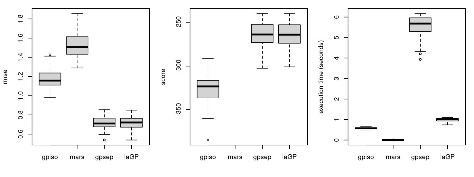
FIGURE 5.12: RMSEs (left), proper scores (middle) and execution times (right) for a bakeoff based on the Friedman data.
MARS is the fastest but least accurate. Library-based GP prediction with laGP is substantially faster than its by-hand analog. Variability in timings is largely due to differing numbers of iterations to convergence when calculating MLEs. Our by-hand separable GP and laGP analog are nearly the same in terms of RMSE and score. However boxplots only summarize marginal results, masking any systematic (if subtle) patterns between comparators over the thirty trials. One advantage to having a randomized experiment where each replicate is trained and tested on the same data is that a paired \(t\)-test can be used to check for systematic differences between pairs of competitors.
##
##  Paired t-test
##
## data:  scores[, 4] and scores[, 3]
## t = -0.79, df = 29, p-value = 0.4
## alternative hypothesis: true mean difference is not equal to 0
## 95 percent confidence interval:
##  -0.8687  0.3839
## sample estimates:
## mean difference
##         -0.2424
The outcome of the test reveals that there’s no difference between these two predictors in terms of accuracy (\(p\)-value greater than the usual 5%). When comparing RMSEs in this way, it may be appropriate to take the log. (Scores are already on a log scale.) So that’s it: now you can try GP regression on data of your own! Of course, there are natural variations we could add to the bakeoff above, such as laGP’s isotropic implementation, and MARS with degree=2. I’ll leave those to the curious reader as a homework exercise (§5.5). You could stop reading now and be satisfied knowing almost all there is to know about deploying GPs in practice.
Or you could let me get a few more words in, since I have your attention. What else is there? We’ve been alluding to “other covariance structures”, so it might be a good idea to be a little more concrete on that. We’ve talked about “properties”, but that’s been vague. Same thing with limitations. We’ll scratch the surface now, and spend whole chapters on that later on. And then there’s the matter of perspective on what a GP is really doing when it’s giving you predictions? Is it really Bayesian?
5.3 Some interpretation and perspective
So we fit some hyperparameters and used MVN conditioning identities to predict. But what are we doing really? Well that depends upon your perspective. I was raised a Bayesian, but have come to view things more pragmatically over the years. There’s a lot you can do with ordinary least squares (OLS) regression, e.g., with the lm command in R. A bespoke fully Bayesian analog might feel like the right thing to do, but represents a huge investment with uncertain reward. Yet there’s value in a clear (Bayesian) chain of reasoning, and the almost automatic regularization that a posterior distribution provides. That is, assuming all calculations are doable, both in terms of coder effort and execution time.
Those “pragmatic Bayesian” perspectives have heavily influenced my view of GP regression, which I’ll attempt to summarize below through a sequence of loosely-connected musings. For those of you who like magic more than mystery, feel free to skip ahead to the next chapter. For those who want lots of theory, try another text. I’m afraid you’ll find the presentation below to be woefully inadequate. For those who are curious, read on.
5.3.1 Bayesian linear regression?
Recall the standard multiple linear regression model, perhaps from your first or second class in statistics.
\[ Y(x) = x^\top \beta + \varepsilon, \quad \varepsilon \stackrel{\mathrm{iid}}{\sim} \mathcal{N}(0, \sigma^2). \]
For \(n\) inputs \(x_1, \dots, x_n\), stacked row-wise into a design matrix \(X_n\), the sampling model may compactly be written as
\[ Y \sim \mathcal{N}_n(X_n \beta, \sigma^2 \mathbb{I}_n). \]
That data-generating mechanism leads to the following likelihood, using observed data values \(Y_n = (y_1, \dots, y_n)^\top\) or RV analogs (for studying sampling distributions):
\[ L(\beta, \sigma^2) = \left(2\pi \sigma^2\right)^{-\frac{n}{2}} \exp \left\{-\frac{1}{2\sigma^2} (Y_n - X_n\beta)^\top (Y_n - X_n\beta) \right\}. \]
Using those equations alone, i.e., only the likelihood, nobody would claim to be positing a Bayesian model for anything. A Bayesian version additionally requires priors on unknown parameters, \(\beta\) and \(\sigma^2\).
So why is it that a slight generalization, obtained by replacing the identity with a covariance matrix parameterized by \(\theta\) and \(g\), and mapping \(\sigma^2 \equiv \tau^2\),
\[ Y \sim \mathcal{N}_n(X_n \beta, \tau^2 K_n), \quad K_n = C_n + g\mathbb{I}_n, \quad C_n^{ij} = C_\theta(x_i, x_j), \]
causes everyone to suddenly start talking about priors over function spaces and calling the whole thing Bayesian? Surely this setup implies a likelihood just as before
\[ L(\beta, \tau^2, \theta, g) = \left(2\pi\tau^2\right)^{-\frac{n}{2}} |K_n|^{-\frac{1}{2}} \exp\left\{-\frac{1}{2\tau^2} (Y_n - X_n\beta)^\top K_n^{-1} (Y_n - X_n\beta) \right\}. \]
We’ve already seen how to infer \(\tau^2\), \(\theta\) and \(g\) hyperparameters – no priors required. Conditional on \(\hat{\theta}\) and \(\hat{g}\)-values, defining \(K_n\), the same MLE calculations for \(\hat{\beta}\) from your first stats class are easy with calculus. See exercises in §5.5. There’s really nothing Bayesian about it until you start putting priors on all unknowns: \(\theta\), \(g\), \(\tau^2\) and \(\beta\). Right?
Not so fast! Here’s my cynical take, which I only halfheartedly believe and will readily admit has as many grains of truth as it has innuendo. Nevertheless, this narrative has some merit as an instructional device, even if a caricature of (a possibly revisionist) history.
First set the stage. The ML community of the mid–late 1990s was enamored with Bayesian learning as an alternative to the prevailing computational learning theory (CoLT) and probably approximately correct (PAC) trends at the time. ML has a habit of appropriating methodology from related disciplines (statistics, operations research, mathematical programming, computer science), usually making substantial enhancements – which are of great value to all, don’t get me wrong – but at the same time re-branding them to the extent that pedigree is all but obscured. One great example is the single-layer perceptron versus logistic regression. Another is active learning versus sequential design, which we shall discuss in more detail in Chapter 6. You have to admit, they’re better at naming things!
Here’s the claim. A core of innovators in ML were getting excited about GPs because they yielded great results for prediction problems in robotics, reinforcement learning, and e-commerce to name a few. Their work led to many fantastic publications, including the text by Rasmussen and Williams (2006) which has greatly influenced my own work, and many of the passages coming shortly. (In many ways, over the years machine learners have made more – and more accessible – advances to the GP arsenal and corpus of related codes than any other community.) I believe that those GP-ML vanguards calculated, possibly subconsciously, that they’d be better able to promote their work to the ML community by dressing it in a fancy Bayesian framework. That description encourages reading with a pejorative tone, but I think this maneuver was largely successful, and those of us who have benefited from their subsequent work owe them a debt of gratitude, because it all could’ve flopped. At that time, in the 1990s, they were hawking humble extensions to old ideas from 1960s spatial statistics, an enterprise that was already in full swing in the computer modeling literature. The decision to push GPs as nonparametric Bayesian learning machines served both as catalyst for enthusiasm in a community that essentially equated “Bayesian” with “better”, and as a feature distinguishing their work from that of other communities who were somewhat ahead of the game, but for whom emphasizing Bayesian perspectives was not as advantageous. That foundation blossomed into a vibrant literature that nearly twenty years later is still churning out some of the best ideas in GP modeling, far beyond regression.
The Bayesian reinterpretation of more classical procedures ended up subsequently becoming a fad in other areas. A great example is the connection between lasso/L1-penalized regression and Bayesian linear modeling with independent double-exponential (Laplace) priors on \(\beta\): the so-called Bayesian lasso (T. Park and Casella 2008). Such procedures had been exposed decades earlier, in less fashionable times (Carlin and Polson 1991) and had been all but forgotten. Discovering that a classical procedure had a Bayesian interpretation, and attaching to it a catchy name, breathed new life into old ideas and facilitated a great many practical extensions.
For GPs that turned out to be a particularly straightforward endeavor. We’ve already seen how to generate \(Y(x)\)’s independent of data, so why not call that a prior? And then we saw how MVN identities could help condition on data, generating \(Y(x) \mid D_n\), so why not call that a posterior? Never mind that we could’ve derived those predictive equations (and we essentially did just that in §5.1) under the “generalized” linear regression model.
But the fact that we can do it, i.e., force a Bayesian GP interpretation, begs three questions.
- What is the prior over?
- What likelihood is being paired with that prior (if not the MVN we’ve been using, which doesn’t need a prior to work magic)?
- What useful “thing” do we extract from this Bayesian enterprise that wasn’t there before?
The answers to those questions lie in the concept of a latent random field.
5.3.2 Latent random field
Another apparatus that machine learners like is graphical models, or diagrammatic depictions of Bayesian hierarchical models. The prevailing such representation for GPs is similar to schematics used to represent hidden Markov models (HMMs). A major difference, however, is that HMMs obey the Markov property, so there’s a direction of flow: the next time step is independent of the past given the current time step. For GPs there’s potential for everything to depend upon (i.e., be correlated with) everything else.

FIGURE 5.13: Diagram of the latent random field; similar to one from Rasmussen and Williams (2006).
The diagram in Figure 5.13 resembles one from Rasmussen and Williams (2006) except it’s more explicit about this interconnectivity. The \(f_i\)-values in the middle row represent a latent Gaussian random field, sitting between inputs \(x_i\) and outputs \(y_i\). They’re latent because we don’t observe them directly, and they’re interdependent on one another. Instead we observe noise-corrupted \(y\)-values, but these are conditionally independent of one another given latent \(f\)-values. The Rasmussen & Williams analog shows these latent \(f\)s residing along a bus, to borrow a computer engineering term, in lieu of the many interconnections shown in Figure 5.13. To emphasize that these latents are unobserved, they reside in dashed/gray rather than solid circles. Interconnections are also dashed/gray, representing unobserved correlations and unobserved noises connecting latents together and linking them with their observed \(y\)-values. The rightmost \((x,f,Y) = (x, f(x), Y(x))\) set of nodes in the figure represent prediction at a new \(x\) location, exhibiting the same degree of interconnectedness and independence in noisy output.
The Bayesian interpretation inherited by the posterior predictive distribution hinges on placing a GP prior on latent \(f_i\)-values, not directly on measured \(y_i\)’s.
\[\begin{equation} F \sim \mathcal{N}_n(0, \tau^2 C_n) \tag{5.15} \end{equation}\]
Above I’m using \(C_n\) rather than \(K_n\) which is our notation for a correlation matrix without nugget. But otherwise this uses our preferred setup from earlier. Since there are no data (\(Y_n\)) values in Eq. (5.15), we can be (more) comfortable about calling this a prior. It’s a prior over latent functions.
Now here’s how the likelihood comes in, so that we’ll have all of the ingredients comprising a posterior: likelihood + prior. Take an iid Gaussian sampling model for \(Y_n \equiv (y_1, \dots, y_n\)) around \(F\):
\[ Y \sim \mathcal{N}_n(F, \sigma^2 \mathbb{I}_n). \]
To map to our earlier notation with a nugget, choose \(\sigma^2 = g \tau^2\). Embellishments may include adding a linear component \(X_n \beta\) into the mean, as \(F + X_n \beta\).
Now I don’t know about you, but to me this looks a little contrived. With prior \(F \mid X_n\) and likelihood \(Y_n \mid F, X_n\), notation for the posterior is \(F \mid D_n\). It’s algebraic form isn’t interesting in and of itself, but an application of Bayes’ rule does reveal a connection to our earlier development.
\[ p(F \mid D_n) = \frac{p(Y_n \mid F, X_n) p(F \mid X_n)}{p(Y_n \mid X_n)} \]
The denominator \(p(Y_n \mid X_n)\) above, for which we have an expression (5.8) in log form, is sometimes called a marginal likelihood or evidence. The former moniker arises from the law of total probability, which allows us to interpret this quantity as arising after integrating out the latent random field \(F\) from the likelihood \(Y_n \mid F, X_n\):
\[ p(Y_n \mid X_n) = \int p(Y_n \mid f, X_n) \cdot p(f \mid X_n) \; df. \]
We only get what we really want, a posterior predictive \(Y(x) \mid D_n = (X_n, Y_n)\), through a different marginalization, this time over the posterior of \(F\):
\[ p(Y(x) \mid D_n) = \int p(Y(x) \mid f) \cdot p(f \mid D_n) \; df. \]
But of course we already have expressions for that as well (5.2). Similar logic, through joint modeling of \(Y_n\) with \(f(x)\), instead of with \(Y(x)\), and subsequent MVN conditioning can be applied to derive \(f(x) \mid D_n\). The result is Gaussian with identical mean \(\mu(x)\), from Eq. (5.2), and variance
\[\begin{equation} \breve{\sigma}^2(x) = \sigma^2(x) - \hat{\tau}^2 \hat{g} = \hat{\tau}^2 (1 - k_n^\top(x) K_n^{-1} k_n(x)). \tag{5.16} \end{equation}\]
Thus, this latent function space interpretation justifies a trick we performed in §5.2.2, when exploring smoothed sinusoid visuals in Figure 5.10. Recall that we obtained de-noised sample paths (gray lines) by omitting the nugget in the predictive variance calculation. This is the same as plugging in \(g=0\) when calculating \(K(\mathcal{X}, \mathcal{X})\), or equivalently using \(C(\mathcal{X}, \mathcal{X})\). At the time we described that maneuver as yielding the epistemic uncertainty – that due to model uncertainty – motivated by a desire for pretty-looking gray lines. In fact, sample paths resulting from that calculation are precisely draws from \(f(\mathcal{X}) \mid D_n\), i.e., posterior samples of the latent function.
Error-bars calculated from that predictive variance are tighter, and characterize uncertainty in predictive mean, i.e., without additional uncertainty coming from a residual sum of squares. Note that \(\hat{g}\) is only removed from the predictive calculation, not from the diagonal of \(K_n\) leading to \(K_n^{-1}\). To make an analogy to linear modeling in R with lm, the former based on \(\sigma^2(x)\) corresponds to interval="prediction", and \(\breve{\sigma}^2(x)\) to interval="confidence" when using predict.lm. (See §3.2.3.) As \(n \rightarrow \infty\), we’ll have that \(\breve{\sigma}^2(x) \rightarrow 0\) for all \(x\), meaning that eventually we’ll learn the latent functions without uncertainty. On the other hand, \(\sigma^2(x)\) could be no smaller than \(\hat{\tau}^2 \hat{g}\), meaning that when it comes to making predictions, they’ll offer an imperfect forecast of the noisy (held-out) response value no matter how much data, \(n\), is available for training.
Was all that worth it? We learned something: predictive distribution \(Y(x) \mid D_n\) involves integrating over a latent function space, at least notionally, even if the requisite calculations and their derivation don’t require working that way. An examination of the properties of those latent functions, or rather correlation functions \(C(\cdot, \cdot)\) which generate those \(f\)’s, could provide insight into the nature of our nonparametric regression. I think that’s the biggest feature of this interpretation.
5.3.3 Stationary kernels
Properties of the correlation function, \(C(x, x')\), or covariance function \(\Sigma(x, x')\), or generically kernel \(k(x, x')\) as preferred in ML, dictate properties of latent functions \(f\). For example, a stationary kernel \(k(x, x')\) is a function only of \(r = x - x'\),
\[ k(x, x') = k(r). \]
More commonly, \(r = |x - x'|\). Our isotropic and separable Gaussian families are both stationary kernels. The most commonly used kernels are stationary, despite the strong restrictions they place on the nature of the underlying process. Characteristics of the function \(f\), via a stationary kernel \(k\), are global since they’re determined only by displacement between coordinates, not positions of the coordinates themselves; they must exhibit the same dynamics everywhere. What, more specifically, are some of the properties of a stationary kernel?
Consider wiggliness, which is easiest to characterize in a single input dimension \(x \in [0,1]\). Define the number of level-\(u\) upcrossings \(N_u\) to be the number of times a random realization of \(f\) crosses level \(u\), from below to above on the \(y\)-axis, when traversing from left to right on the \(x\)-axis. It can be shown that the expected number of level-\(u\) upcrossings under a stationary kernel \(k(\cdot)\) is
\[\begin{equation} \mathbb{E}\{N_u \} = \frac{1}{2\pi} \sqrt{\frac{-k''(0)}{k(0)}} \exp \left( - \frac{u^2}{2 k(0)} \right). \tag{5.17} \end{equation}\]
For a Gaussian kernel, the expected number of zero-crossings (i.e., \(u=0\)) works out to be
\[ \mathbb{E}\{N_0 \} \propto \theta^{-1/2}. \]
See Adler (2010) for more details. Hyperparameter \(\theta\) appears in the denominator of squared distance, so on the scale of inputs \(x\), i.e., “un-squared” distance, \(\theta\) is proportional to the expected length in the input space before crossing zero: hence the name characteristic lengthscale. Therefore \(\theta\) directly controls how often latent functions change direction, which they must do in order to cross zero more than once (from below). A function with high \(\mathbb{E}\{N_u \}\), which comes from small \(\theta\), would have more bumps, which we might colloquially describe as more wiggly. The same result can be applied separately in each coordinate direction of a separable Gaussian kernel using \(\theta_k\), for all \(k=1,\dots,m\).
Consider smoothness, in the calculus sense – not as the opposite of wiggliness. A Gaussian kernel is infinitely differentiable, which in turn means that its latent \(f\) process has mean-square derivatives of all orders, and this is very smooth. Not many physical phenomena – think back to your results from Physics 101 or a first class in differential equations – are infinitely smooth. Despite this not being realistic for most real-world processes, (separable) Gaussian kernels are still the most widely used. Why? Because they’re easy to code up; GPs are relatively robust to misspecifications, within reason (remember what happened when we forced \(\tau^2 = 1\)); faults of infinite smoothness are easily masked by “fudges” already present in the model for other reasons, e.g., with nugget or jitter (Andrianakis and Challenor 2012; Gramacy and Lee 2012; Peng and Wu 2014). And finally there’s the practical matter of guaranteeing a proper, positive definite covariance regardless of input dimension.
If a Gaussian kernel isn’t working well, or if you want finer control on mean-square differentiability, then consider a Matérn family member, with
\[ k_\nu(r) = \frac{2^{1-\nu}}{\Gamma(\nu)} \left(r\sqrt{\frac{2\nu}{\theta}} \right)^\nu K_\nu \left(r\sqrt{\frac{2\nu}{\theta}} \right). \]
Above \(K_\nu\) is a modified Bessel function of the second kind, \(\nu\) controls smoothness, and \(\theta\) is a lengthscale as before. As \(\nu \rightarrow \infty\), i.e., a very smooth parameterization, we get
\[ k_\nu(r) \rightarrow k_{\infty}(r) = \exp \left\{-\frac{r^2}{2\theta} \right\} \]
which can be recognized as (a re-parameterized) Gaussian family, where \(r\) is measured on the scale of ordinary (not squared) Euclidean distances.
The code below sets up this “full” Matérn in R so we can play with it a little.
matern <- function(r, nu, theta)
 {
  rat <- r*sqrt(2*nu/theta)
  C <- (2^(1 - nu))/gamma(nu) * rat^nu * besselK(rat, nu)
  C[is.nan(C)] <- 1
  return(C)
 }
Sample paths of latent \(f\) under a GP with this kernel will be \(k\) times differentiable if and only if \(\nu > k\). Loosely speaking this means that sample paths from smaller \(\nu\) will be rougher than those from larger \(\nu\). This is quite surprising considering how similar the kernel looks when plotted for various \(\nu\), as shown in Figure 5.14.
r <- seq(eps, 3, length=100)
plot(r, matern(r, nu=1/2, theta=1), type="l", ylab="k(r,nu)")
lines(r, matern(r, nu=2, theta=1), lty=2, col=2)
lines(r, matern(r, nu=10, theta=1), lty=3, col=3)
legend("topright", c("nu=1/2", "n=2", "nu=10"), lty=1:3, col=1:3, bty="n")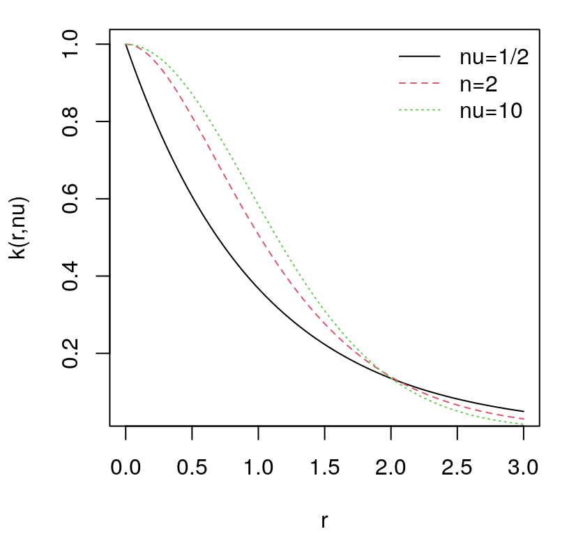
FIGURE 5.14: Matérn kernels versus Euclidean distance.
In all three cases the lengthscale parameter is taken as \(\theta=1\). R code below calculates covariance matrices for latent field draws \(F\) under these three Matérn specifications. Careful, as in the discussion above, the matern function expects its r input to be on the scale of ordinary (not squared) distances.
X <- seq(0, 10, length=100)
R <- sqrt(distance(X))
K0.5 <- matern(R, nu=1/2, theta=1)
K2 <- matern(R, nu=2, theta=1)
K10 <- matern(R, nu=10, theta=1) + diag(eps, 100)
Notice that we’re not augmenting the diagonal of these matrices with \(\epsilon\) jitter. One of the great advantages to a Matérn (for small \(\nu\)) is that it creates covariance matrices that are better conditioned, i.e., farther from numerically non-positive definite. Using those covariances, Figure 5.15 plots three sample paths for each case.
par(mfrow=c(1,3))
matplot(X, t(rmvnorm(3,sigma=K0.5)), type="l", col=1, lty=1,
  xlab="x", ylab="y, nu=1/2")
matplot(X, t(rmvnorm(3,sigma=K2)), type="l", col=2, lty=2,
  xlab="x", ylab="y, nu=2")
matplot(X, t(rmvnorm(3,sigma=K10)), type="l", col=3, lty=3, xlab="x",
  ylab="y, nu=10")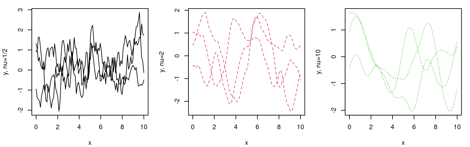
FIGURE 5.15: Sample paths under Matérn kernels with \(\nu = 0.5\) (left), \(\nu=2\) (middle) and \(\nu=10\) (right).
Surfaces under \(\nu=1/2\), shown on the left, are very rough. Since \(\nu < 1\) they’re nowhere differentiable, yet they still have visible correlation in space. On the right, where \(\nu = 10\), surfaces are quite smooth; ones which are nine-times differentiable. In the middle is an intermediate case which is smoother than the first one (being once differentiable) but not as smooth as the last one. To get a sense of what it means to be just once differentiable, as in the middle panel of the figure, consider the following first and second numerical derivatives (via first differences) for a random realization when \(\nu = 2\).
F <- rmvnorm(1, sigma=K2)
dF <- (F[-1] - F[-length(F)])/(X[2] - X[1])
d2F <- (dF[-1] - dF[-length(dF)])/(X[2] - X[1])
Figure 5.16 plots these three sets of values on a common \(x\)-axis.
plot(X, F, type="l", lwd=2, xlim=c(0,13), ylim=c(-5,5),
  ylab="F and derivatives")
lines(X[-1], dF, col=2, lty=2)
lines(X[-(1:2)], d2F, col=3, lty=3)
legend("topright", c("F", "dF", "d2F"), lty=1:3, col=1:3, bty="n")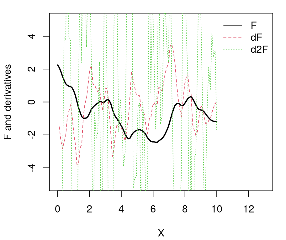
FIGURE 5.16: Numerical derivatives for Matérn sample paths.
Whereas the original function realization F seems reasonably smooth, its first differences dF are jagged despite tracing out a clear spatial pattern in \(x\). Since first differences are not smooth, second differences d2F are erratic: this random latent function realization is not twice differentiable. Of course, these are all qualitative statements based on finite realizations, but you get the gist.
We’re not usually in the business of generating random (latent) functions. Rather, given observed \(y\)-values we wish to estimate the unknown latent function \(f\) via a choice of correlation family, and settings for its hyperparameters. What does this mean for \(\nu\), governing smoothness? Some of the biggest advocates for the Matérn, e.g., Stein (2012), argue that you should learn smoothness, \(\nu\), from your training data. But that’s fraught with challenges in practice, the most important being that noisy data provide little guidance for separating noise from roughness, which under the Matérn is regarded as a form of signal. This results in a likelihood surface which has many dead (essentially flat) spots. More typically, the degree of smoothness is regarded as a modeling choice, ideally chosen with knowledge of underlying physical dynamics.
Another challenge involves the Bessel function \(K_\nu\), the evaluation of which demands a cumbersome numerical scheme (say using besselK in R) applied repeatedly to \(\mathcal{O}(n^2)\) pairs of distances \(r\) between training data inputs \(X_n\). For most moderate data sizes, \(n < 1000\) say, creating an \(n \times n\) covariance matrix under the Matérn is actually slower than decomposing it, despite the \(\mathcal{O}(n^3)\) cost that this latter operation implies.
A useful re-formulation arises when \(\nu = p + \frac{1}{2}\) for non-negative integer \(p\), in which case \(p\) exactly determines the number of mean-square derivatives.
\[ k_{\nu=p+\frac{1}{2}}(r) = \exp \left\{r\sqrt{\frac{2\nu}{\theta}} \right\} \frac{\Gamma(p+1)}{\Gamma(2p+1)} \sum_{i=0}^p \frac{(p+i)!}{i!(p-i)!} \left(r\sqrt{\frac{8\nu}{\theta}}\right)^{p-i} \]
Whether or not this is simpler than the previous specification is a matter of taste. From this version it’s apparent that the kernel is comprised of a product of an exponential and a polynomial of order \(p\). Although tempting to perform model search over discrete \(p\), this is not any easier than over continuous \(\nu\). However it is easier to deduce the form from more transparent and intuitive components (i.e., no Bessel functions), at least for small \(p\). Choosing \(p = 0\), yielding only the exponential part which is equivalent to \(k(r) = e^{-\frac{r^2}{\theta}}\), is sometimes referred to as the exponential family. This choice is also a member of the power exponential family, introduced in more detail momentarily. We’ve already discussed how \(p=0\), implying \(\nu = 1/2\), is appropriate for rough surfaces. At the risk of being even more redundant, \(p \rightarrow \infty\) is a great choice when dynamics are super smooth, although clearly having an infinite sum isn’t practical for implementation. From a technical standpoint, both choices are probably too rough or too smooth, respectively, even though they (especially the Gaussian) work fine in many contexts, to the chagrin of purists.
Entertaining a middle ground has its merits. Practically speaking, without explicit knowledge about higher-order derivatives, it’ll be hard to distinguish between values \(\nu \geq 7/2\), meaning \(p \geq 3\), and much larger settings (\(p,\nu \rightarrow \infty\)) especially with noisy data. That leaves essentially two special cases, which emit relatively tidy expressions:
\[\begin{align} && k_{3/2}(r) &= \left(1 + r\sqrt{\frac{3}{\theta}} \right) \exp \left(- r\sqrt{\frac{3}{\theta}} \right) \tag{5.18} \\ \mbox{or } && k_{5/2}(r) &= \left(1 + r\sqrt{\frac{5}{\theta}} + \frac{5r^2}{3\theta} \right) \exp \left(- r\sqrt{\frac{5}{\theta}} \right). \notag \end{align}\]
The advantage of these cases is that there are no Bessel functions, no sums of factorials nor fractions of gammas. Most folks go for the second one (\(p=2\)) without bothering to check against the first, perhaps appealing to physical intuition that many interesting processes are at least twice differentiable. Worked examples with these choices are deferred to Chapter 10 on replication and heteroskedastic modeling. In the meantime, the curious reader is invited to explore them in a homework exercise in §5.5.
The power exponential family would, at first blush, seem to have much in common with the Matérn,
\[ k_\alpha (r) = \exp \left\{- \left(\frac{r}{\sqrt{\theta}}\right)^\alpha \right\} \quad \mbox{ for } 0 < \alpha \leq 2, \] having the same number of hyperparameters and coinciding on two special cases \(\alpha = 1 \Leftrightarrow p=0\) and \(\alpha = 2 \Leftrightarrow p \rightarrow \infty\). An implementation in R is provided below.
powerexp <- function(r, alpha, theta)
 {
  C <- exp(-(r/sqrt(theta))^alpha)
  C[is.nan(C)] <- 1
  return(C)
 }
However the process is never mean-square differentiable except in the Gaussian (\(\alpha = 2\)) special case. Whereas the Matérn offers control over smoothness, a power exponential provides essentially none. Yet both offer potential for greater numerical stability, owing to better covariance matrix condition numbers, than their Gaussian special cases. A common kludge is to choose \(\alpha = 1.9\) in lieu of \(\alpha = 2\) with the thinking that they’re “close” (which is incorrect) but the former is better numerically (which is correct). As with Matérn \(\nu\), or perhaps even more so, it’s surprising that fine variation in a single hyperparameter (\(\alpha\)) can have such a profound effect on the resulting latent functions, especially when their kernels look so similar as a function of \(r\). See Figure 5.17.
plot(r, powerexp(r, alpha=1.5, theta=1), type="l", ylab="k(r,alpha)")
lines(r, powerexp(r, alpha=1.9, theta=1), lty=2, col=2)
lines(r, powerexp(r, alpha=2, theta=1), lty=3, col=3)
legend("topright", c("alpha=1.5", "alpha=1.9", "alpha=2"),
  lty=1:3, col=1:3, bty="n")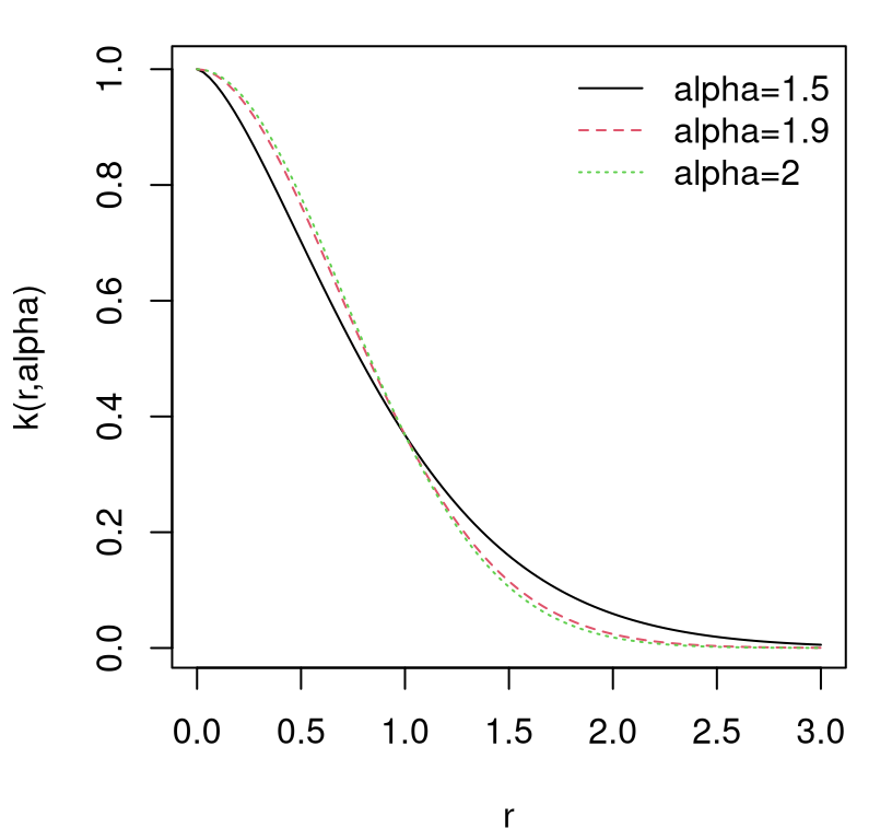
FIGURE 5.17: Power exponential kernels versus Euclidean distance.
Despite the strong similarity for \(\alpha \in \{1.5, 1.9, 2\}\) in kernel evaluations, the resulting sample paths exhibit stark contrast, as shown in Figure 5.18.
Ka1.5 <- powerexp(R, alpha=1.5, theta=1)
Ka1.9 <- powerexp(R, alpha=1.9, theta=1)
Ka2 <- powerexp(R, alpha=2, theta=1) + diag(eps, nrow(R))
par(mfrow=c(1,3))
ylab <- paste0("y, alpha=", c(1.5, 1.9, 2))
matplot(X, t(rmvnorm(3, sigma=Ka1.5)), type="l", col=1, lty=1,
  xlab="x", ylab=ylab[1])
matplot(X, t(rmvnorm(3, sigma=Ka1.9)), type="l", col=2, lty=2,
  xlab="x", ylab=ylab[2])
matplot(X, t(rmvnorm(3, sigma=Ka2)), type="l", col=3, lty=3,
  xlab="x", ylab=ylab[3])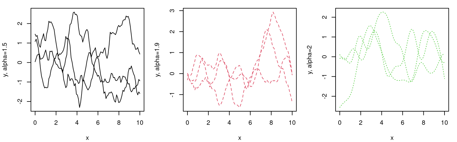
FIGURE 5.18: Sample paths under power exponential kernels with \(\alpha = 1.5\) (left), \(\alpha=1.9\) (middle) and \(\alpha=2\) (right).
The \(\alpha = 2\) case is a special one: very smooth latent function realizations. Although \(\alpha = 1.9\) is not as rough as \(\alpha = 1.5\), it still exhibits “sharp turns”, albeit fewer. That pair are more similar to one another in that respect than either is to the final one where \(\alpha = 2\), being infinitely smooth.
The rational quadratic kernel
\[ k_{\mathrm{rq}} (r) = \left(1 + \frac{r^2}{2\alpha \theta } \right)^{-\alpha} \quad \mbox{ with } \alpha > 0 \]
can be derived as a scale mixture of Gaussian (power exponential with \(\alpha = 2\)) and exponential (power exponential with \(\alpha = 1\)) kernels over \(\theta\). Since that mixture includes the Gaussian, the process is infinitely mean-square differentiable for all \(\alpha\). An implementation of this kernel in R is provided below.
ratquad <- function(r, alpha, theta)
 {
  C <- (1 + r^2/(2 * alpha * theta))^(-alpha)
  C[is.nan(C)] <- 1
  return(C)
 }
To illustrate, panels of Figure 5.19 show the kernel (left) and three MVN realizations (right) for each \(\alpha \in \{1/2, 2, 10\}\).
par(mfrow=c(1,2))
plot(r, ratquad(r, alpha=1/2, theta=1), type="l",
  ylab="k(r,alpha)", ylim=c(0,1))
lines(r, ratquad(r, alpha=2, theta=1), lty=2, col=2)
lines(r, ratquad(r, alpha=10, theta=1), lty=3, col=3)
legend("topright", c("alpha=1/2", "alpha=2", "alpha=10"), lty=1:3,
  col=1:3, bty="n")
Eps <- diag(eps, nrow(R))
plot(X, rmvnorm(1, sigma=ratquad(R, alpha=1/2, theta=1) + Eps), type="l",
  col=1, lty=1, xlab="x", ylab="y", ylim=c(-2.5,2.5))
lines(X, rmvnorm(1, sigma=ratquad(R, alpha=2, theta=1) + Eps), col=2, lty=2)
lines(X, rmvnorm(1, sigma=ratquad(R, alpha=10, theta=1) + Eps), type="l",
  col=3, lty=3)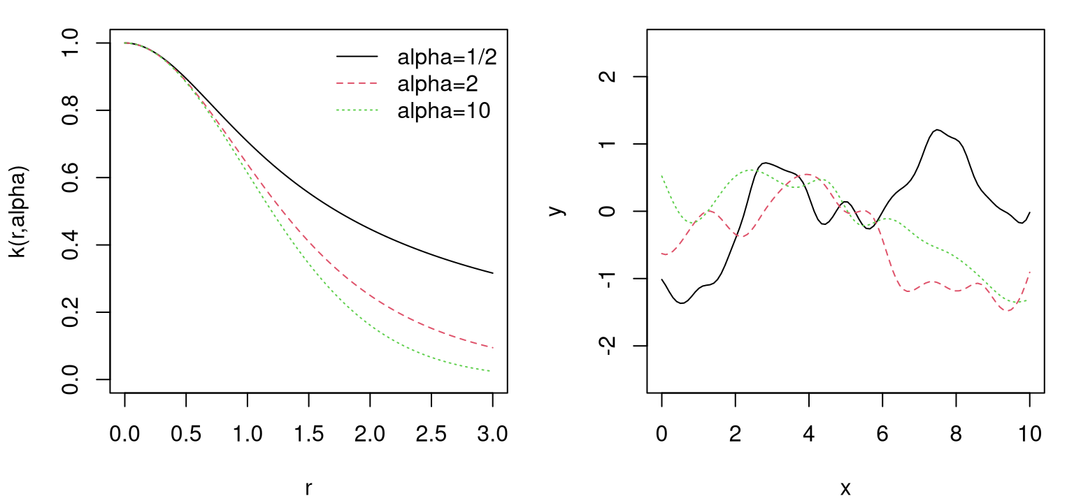
FIGURE 5.19: Rational quadratic kernel evaluations (left) and paths (right).
Although lower \(\alpha\) yield rougher characteristics, all are smooth compared to their non-differential analogs introduced earlier.
The idea of hybridizing two kernels, embodied in the particular by the rational quadratic kernel above, nicely generalizes. Given two well-defined kernels, i.e., generating a positive definite covariance structure, there are many ways they can be combined into a single well-defined kernel. The sum of two kernels is a kernel. In fact, if \(f(x) = \sum f_k(x_k)\), for random \(f_k(x_k)\) with univariate kernels, then the kernel of \(f(x)\) arises as the sum of those kernels. Durrande, Ginsbourger, and Roustant (2012) show how such an additive GP-modeling approach can be attractive in high input dimensions. A product of two kernels is a kernel. The kernel of a convolution is the convolution of the kernel. Anisotropic versions of isotropic covariance functions can be created through products, leading to a separable formulation, or through quadratic forms like \(r^2(x, x') = (x - x')^\top A (x - x')\) where \(A\) may augment the hyperparameter space. Low rank \(A\) are sometimes used to implement linear dimensionality reduction. Rank one choices of \(A\) lead to what are known as GP single-index models [GP-SIMs; Gramacy and Lian (2012)].
Although somewhat less popular, there are stationary kernels which are common in specialized situations such as with spherical input coordinates, or for when periodic effects are involved. A good reference for these and several others is an unpublished manuscript by Abrahamsen (1997). Another good one is Wendland (2004), particularly Chapter 9, which details piecewise polynomial kernels with compact support, meaning that they go exactly to zero which can be useful for fast computation with sparse linear algebra libraries. The kergp package (Deville, Ginsbourger, and Roustant 2018) on CRAN provides a nice interface for working with GPs under user-customized kernels.
Kernels supporting qualitative factors, i.e., categorical and ordinal inputs, and mixtures thereof with ordinary continuous ones, have appeared in the literature. See work by Qian, Wu, and Wu (2008), Zhou, Qian, and Zhou (2011) and a recent addition from Y. Zhang et al. (2018). None of these ideas have made their way into public software, to my knowledge. The tgp package supports binarized categorical inputs through treed partitioning. More detail is provided in §9.2.2.
It’s even possible to learn all \(n(n-1)/2\) entries of the covariance matrix separately, under regularization and a constraint that the resulting \(\Sigma_n\) is positive definite, with semidefinite programming. Lanckriet et al. (2004) describe a transductive learner that makes this tractable implicitly, through the lens of prediction at a small number of testing sites. We’ll take a similar approach to thrifty approximation of more conventional GP learning in §9.3.
This section was titled “Stationary kernels”. Convenient nonstationary GP modeling is deferred to Chapter 9, however it’s worth closing with some remarks connecting back to those made along with linear modeling in §5.3.1 using some simple, yet nonstationary kernel specifications. It turns out that there are choices of kernel which recreate linear and polynomial (mean) modeling.
\[ \begin{aligned} \mbox{linear } && k(x, x') &= \sum_{k=1}^m \beta_k x_k x_k' \\ \mbox{polynomial } && k(x, x') &= (x^\top x' + \beta)^p \end{aligned} \]
Here \(\beta\) is vectorized akin to linear regression coefficients, although there’s no direct correspondence. These kernels cannot be rewritten in terms of displacement \(x - x'\) alone. However, their latent function realizations are not nonstationary in a way that many regard in practice as genuine because, as linear and polynomial models, their behavior is rigidly rather than flexibly defined. In other words, the nature of nonstationarity is prescribed rather than emergent in the data-fitting process. The fact that you can do this – choose a kernel to encode mean structure in the covariance – lends real credence to the characterization “it’s all in the covariance” when talking about GP models. You can technically have a zero-mean GP with a covariance structure combining linear and spatial structures through sums of kernels, but you’d only do that if you’re trying to pull the wool over someone’s eyes. (Careful not to do it to yourself.) Most folks would sensibly choose the more conventional model of linear mean and spatial (stationary) covariance. But the very fact that you can do it again begs the question: why get all Bayesian about the function space? If an ordinary linear model – which is not typically thought of as Bayesian without additional prior structure – arises as a special choice of kernel, then why should introduction of a kernel automatically put us in a Bayesian state of mind?
GP regression is just multivariate normal modeling, and you can get as creative as you want with mean and covariance. There are some redundancies, as either can implement linear and polynomial modeling, and much more. Sometimes you know something about prevailing input–output relationships, and for those settings GPs offer potential to tailor as a means of spatial regularization, which is a classical statistician’s roundabout way of saying “encode prior beliefs”. For example, if \(a(x)\) is a known deterministic function and \(g(x) = a(x) f(x)\), where \(f(x)\) is a random process, then \(\mathbb{C}\mathrm{ov}(g(x), g(x')) = a(x) k(x, x') a(x')\). This can be used to normalize kernels by choosing \(a(x) = k^{-1/2}(x,x)\) so that
\[ \bar{k}(x, x') = \frac{k(x,x')}{\sqrt{k(x,x)}\sqrt{k(x',x')}}. \]
That’s a highly stylized example which is not often used in practice, yet it offers a powerful testament to potential for GP customization. GP regression can either be out-of-the-box with simple covariance structures implemented by library subroutines, ready for anything, or can be tailored to the bespoke needs of a particular modeling enterprise and data type. You can get very fancy, or you can simplify, and inference for unknowns need not be too onerous if you stick to likelihood-based criteria paired with mature libraries for optimization with closed-form derivatives.
5.3.4 Signal-to-noise
As with any statistical model, you have to be careful not to get too fancy or it may come back to bite you. The more hyperparameters purporting to offer greater flexibility or a better-tuned fit, the greater the estimation risk. By estimation risk I mean both potential to fit noise as signal, as well as its more conventional meaning (particularly popular in empirical finance) which fosters incorporation of uncertainties, inherent in high variance sampling distributions for optimized parameters, that are often overlooked. Nonparametric models and latent function spaces exacerbate the situation. Awareness of potential sources of such risk is particularly fraught, and assessing its extent even more so. At some point there might be so many knobs that its hard to argue that the “hyperparameter” moniker is apt compared to the more canonical “parameter”, giving the practitioner the sense that choosing appropriate settings is key to getting good fits.
To help make these concerns a little more concrete, consider the following simple data generating mechanism
\[\begin{equation} f(x) = \sin(\pi x/5) + 0.2\cos(4 \pi x/5), \tag{5.19} \end{equation}\]
originally due to Higdon (2002). Code below observes that function with noise on an \(n=40\) grid.
x <- seq(0, 10, length=40)
ytrue <- (sin(pi*x/5) + 0.2*cos(4*pi*x/5))
y <- ytrue + rnorm(length(ytrue), sd=0.2)
The response combines a large amplitude periodic signal with another small amplitude one that could easily be confused as noise. Rather than shove these data pairs into a GP MLE subroutine, consider instead a grid of lengthscale and nugget values.
Below the MVN log likelihood is calculated for each grid pair, and the corresponding predictive equations evaluated at a second grid of \(\mathcal{X} \equiv\) xx inputs, saved for each hyperparameter pair on the first, hyperparameter grid.
ll <- rep(NA, nrow(grid))
xx <- seq(0, 10, length=100)
pm <- matrix(NA, nrow=nrow(grid), ncol=length(xx))
psd <- matrix(NA, nrow=nrow(grid), ncol=length(xx))
for(i in 1:nrow(grid)) {
  gpi <- newGP(matrix(x, ncol=1), y, d=grid[i,1], g=grid[i,2])
  p <- predGP(gpi, matrix(xx, ncol=1), lite=TRUE)
  pm[i,] <- p$mean
  psd[i,] <- sqrt(p$s2)
  ll[i] <- llikGP(gpi)
  deleteGP(gpi)
}
l <- exp(ll - max(ll))
The code above utilizes isotropic (newGP/predGP) GP functions from laGP. Since the data is in 1d, these are equivalent to separable analogs illustrated earlier in §5.2.6. For now, concentrate on (log) likelihood evaluations; we’ll come back to predictions momentarily. Figure 5.20 shows the resulting likelihood surface as an image in the \(\theta \times g\) plane. Notice that the final line in the code above exponentiates the log likelihood, so the figure is showing \(z\)-values (via color) on the likelihood scale.
image(theta, g, matrix(l, ncol=length(theta)), col=cols)
contour(theta, g, matrix(l, ncol=length(g)), add=TRUE)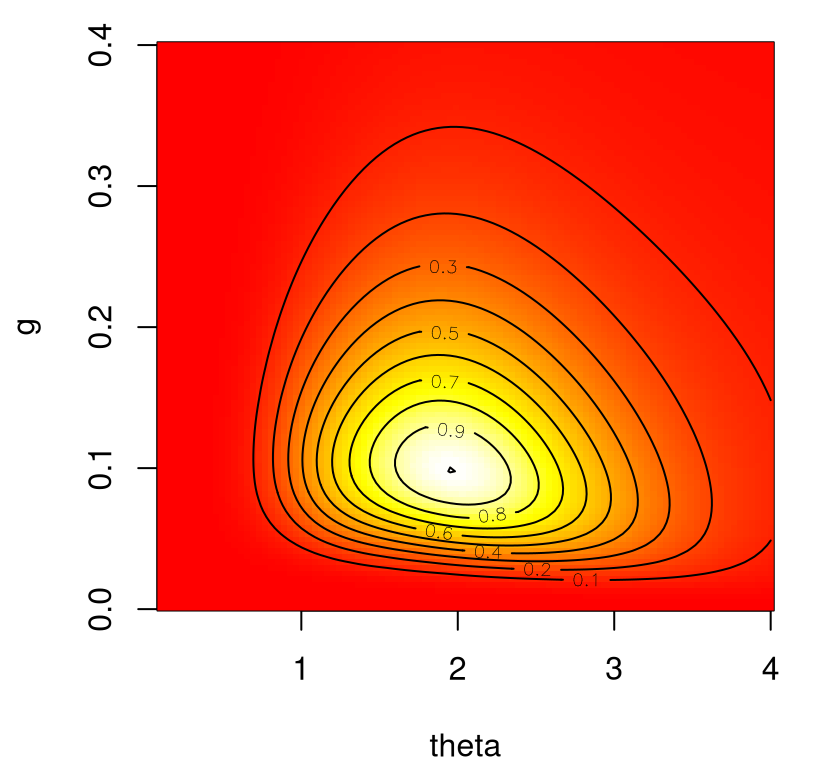
FIGURE 5.20: Log likelihood surface over lengthscale \(\theta\) and nugget \(g\) for mixed sinusoid data (5.19).
Since the data is random, it’s hard to anticipate an appropriate range for \(\theta\) and \(g\) axes. It’s worth repeating these codes in your own R session to explore variations that arise under new datasets generated under novel random noise, adding another layer to the sense of estimation risk, i.e., beyond that which is illustrated here. What can be seen in Figure 5.20? Maybe it looks like an ordinary log likelihood surface in 2d: pleasantly unimodal, convex, etc., and easy to maximize by eyeball norm. (Who needs fancy numerical optimizers after all?) There’s some skew to the surface, perhaps owing to positivity restrictions placed on both hyperparameters.
In fact, that skewness is hiding a multimodal posterior distribution over functions. The modes are “higher signal/lower noise” and “lower signal/higher noise”. Some random realizations reveal this feature through likelihood more than others, which is one reason why repeating this in your own session may be helpful. Also keep in mind that there’s actually a third hyperparameter, \(\hat{\tau}^2\), being optimized implicitly through the concentrated form of the log likelihood (5.8). So there’s really a third dimension to this view which is missing, challenging a more precise visualization and thus interpretation. Such signal–noise tension is an ordinary affair, and settling for one MLE tuple in a landscape of high values – even if you’re selecting the very highest ones – can grossly underestimate uncertainty. What is apparent in Figure 5.20 is that likelihood contours trace out a rather large area in hyperparameter space. Even the red “outer-reaches” in the viewing area yield non-negligible likelihood, which is consistent across most random realizations. This likelihood surface is relatively flat.
The best view of signal-to-noise tension is through the predictive surface, in particular what that surface would look like for a multitude of most likely hyperparameter settings. To facilitate that, code below pre-calculates quantiles derived from predictive equations obtained for each hyperparameter pair.
Figure 5.21 shows three sets of lines (mean and quantile-based interval) for every hyperparameter pair, but not all lines are visualized equally. Transparency is used to downweight low likelihood values. Multiple low likelihood settings accumulate shading, when the resulting predictive equations more or less agree, and gain greater opacity.
plot(x,y, ylim=c(range(q1, q2)))
matlines(xx, t(pm), col=rgb(0,0,0,alpha=(l/max(l))/2), lty=1)
matlines(xx, t(q1), col=rgb(1,0,0,alpha=(l/max(l))/2), lty=2)
matlines(xx, t(q2), col=rgb(1,0,0,alpha=(l/max(l))/2), lty=2)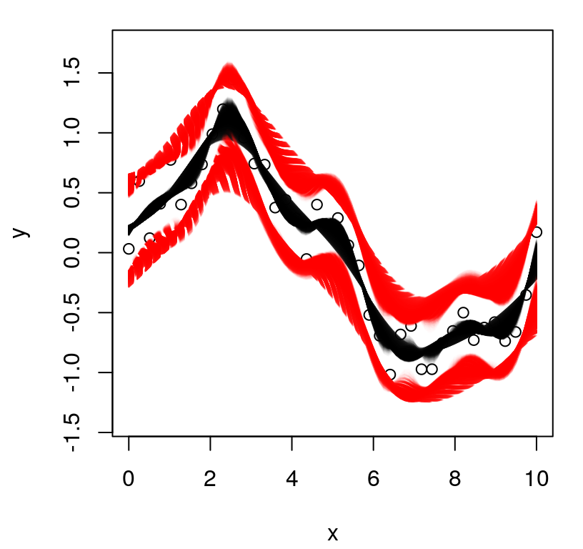
FIGURE 5.21: Posterior predictive equations in terms of means (solid-black) and quantiles (dashed-red).
The hyperparameter grid is \(100 \times 100\), but clearly there are not \(3 \times 10000\) distinct lines visible in the figure. Nevertheless it’s easy to see two regimes. Some of the black/red lines are more wavy, explaining the low-amplitude periodic structure as signal; others are less wavy, explaining it as noise. Although the likelihood was unimodal, we have a multimodal posterior predictive surface.
For all the emphasis on a Bayesian perspective, marginalizing over latent functions and whatever, it’s surprising that Bayesian inference is rarely used where it’s needed most. Clearly the MLE/MAP is missing an important element of uncertainty. Only fully Bayesian posterior inference, after specifying priors on hyperparameters and running Markov chain Monte Carlo (MCMC) for posterior sampling, could provide a full assessment of estimation risk and provide posterior predictive quantities with full UQ. Very few libraries offer this functionality, tgp, spBayes and plgp being three important exceptions, yet these rely on rather conventional covariance specifications. The tgp package has some extra, highly non-standard, features which will be discussed in more detail in §9.2.2. As covariance kernels incorporate more hyperparameters – smoothness, separable vectorized lengthscales, rank-one anisotropy, latent noise structures (Chapter 10), whatever Franken-kernel results from adding/convolving/multiplying – and likewise incorporate well-thought-out parametric mean structures, it’s obvious that a notionally nonparametric GP framework can become highly and strongly parameterized. In such settings, one must be very careful not to get overconfident about point-estimates so-derived. The only way to do it right, in my opinion, is to be fully Bayesian.
With that in mind, it’s a shame to give the (at worst false, at best incomplete) impression of being Bayesian without having to do any of those things. In that light, ML marketing of GPs as Bayesian updating is a double-edged sword. Just because something can be endowed with a Bayesian interpretation, doesn’t mean that it automatically inherits all Bayesian merits relative to a more classical approach. A new ML Bayesian perspective on kriging spawned many creative ideas, but it was also a veneer next to the real thing.
5.4 Challenges and remedies
This final section wraps up our GP chapter on somewhat of a lower note. GPs are remarkable, but they’re not without limitations, the most limiting being computational. In order to calculate \(K_n^{-1}\) and \(|K_n|\) an \(\mathcal{O}(n^3)\) decomposition is required for dense covariance matrices \(K_n\), as generated by most common kernels. In the case of MLE inference, that limits training data sizes to \(n\) in the low thousands, loosely, depending on how many likelihood and gradient evaluations are required to perform numerical maximization. You can do a little better with the right linear algebra libraries installed. See Appendix A.1 for details. (It’s easier than you might think.)
Fully Bayesian GP regression, despite many UQ virtues extolled above, can all but be ruled out on computational grounds when \(n\) is even modestly large (\(n > 2000\) or so), speedups coming with fancy matrix libraries notwithstanding. If it takes dozens or hundreds of likelihood evaluations to maximize a likelihood, it will take several orders of magnitude more to sample from a posterior by MCMC. Even in cases where MCMC is just doable, it’s sometimes not clear that posterior inference is the right way to spend valuable computing resources. Surrogate modeling of computer simulation experiments is a perfect example. If you have available compute cycles, and are pondering spending them on expensive MCMC to better quantify uncertainty, why not spend them on more simulations to reduce that uncertainty instead? We’ll talk about design and sequential design in the next two chapters.
A full discussion of computational remedies, which mostly boils down to bypassing big matrix inverses, will be delayed until Chapter 9. An exception is GP approximation by convolution which has been periodically revisited, over the years, by geostatistical and computer experiment communities. Spatial and surrogate modeling by convolution can offer flexibility and speed in low input dimension. Modern versions, which have breathed new life into geospatial (i.e., 2d input) endeavours by adding multi-resolution features and parallel computing (Katzfuss 2017), are better reviewed in another text. With emphasis predominantly being on modestly-larger-dimensional settings common in ML and computer surrogate modeling contexts, the presentation here represents somewhat of a straw man relative to Chapter 9 contributions. More favorably said: it offers another perspective on, and thus potentially insight into, the nature of GP regression.
5.4.1 GP by convolution
In low input dimension it’s possible to avoid decomposing a big covariance matrix and obtain an approximate GP regression by taking pages out of a splines/temporal modeling play-book. Higdon (2002) shows that one may construct a GP \(f(x)\) over a general region \(x \in \mathcal{X}\) by convolving a continuous Gaussian white noise process \(\beta(x)\) with smoothing kernel \(k(x)\):
\[\begin{equation} f(x) = \int_{\mathcal{X}} k(u - x) \beta(u) \; du, \quad \mbox{for } x \in \mathcal{X}. \tag{5.20} \end{equation}\]
The resulting covariance for \(f(x)\) depends only on relative displacement \(r=x - x'\):
\[ c(r) = \mathbb{C}\mathrm{ov}(f(x), f(x')) = \int_{\mathcal{X}} k(u-x)k(u-x') \; du = \int_{\mathcal{X}} k(u-r) k(u)\; du. \]
In the case of isotropic \(k(x)\) there’s a 1:1 equivalence between smoothing kernel \(k\) and covariance kernel \(c\).
\[ \mbox{e.g., } \quad k(x) \propto \exp\left\{-\frac{1}{2} \left\Vert x \right\Vert^2 \right\} \rightarrow c(r) \propto \exp\left\{-\frac{1}{2} \left\Vert\frac{r}{2}\right\Vert^2 \right\}. \]
Note the implicit choice of lengthscale exhibited by this equivalence.
This means that rather than defining \(f(x)\) directly through its covariance function, which is what we’ve been doing in this chapter up until now, it may instead be specified indirectly, yet equivalently, through the latent a priori white noise process \(\beta(x)\). Sadly, the integrals above are not tractable analytically. However by restricting the latent process \(\beta(x)\) to spatial sites \(\omega_1, \dots, \omega_m\), we may instead approximate the requisite integral with a sum. Like knots in splines, the \(\omega_j\) anchor the process at certain input locations. Bigger \(m\) means better approximation but greater computational cost.
Now let \(\beta_j = \beta(\omega_j)\), for \(j=1,\dots,\ell\), and the resulting (approximate yet continuous) latent function under GP prior may be constructed as
\[ f(x) = \sum_{j=1}^\ell \beta_j k(x - \omega_j), \]
where \(k(\cdot - \omega_j)\) is a smoothing kernel centered at \(\omega_j\). This \(f\) is a random function because the \(\beta_j\) are random variables. Choice of kernel is up to the practitioner, with the Gaussian above being a natural default. In spline/MARS regression, a “hockey-stick” kernel \(k(\cdot - \omega_j) = (\cdot - \omega_i)_{+} \equiv (\cdot - \omega_j) \cdot \mathbb{I}_{\{\cdot - \omega_j > 0\}}\) is a typical first choice.
For a concrete example, here’s how one would generate from the prior under this formulation, choosing a normal density with mean zero and variance one as kernel and an evenly spaced grid of \(\ell=10\) locations \(\omega_j\), \(j=1,\dots,\ell\). It’s helpful to have the knot grid span a slightly longer range in the input domain (e.g., about 10% bigger) than the desired range for realizations.
ell <- 10
n <- 100
X <- seq(0, 10, length=n)
omega <- seq(-1, 11, length=ell)
K <- matrix(NA, ncol=ell, nrow=n)
for(j in 1:ell) K[,j] <- dnorm(X, omega[j])
The last line in the code above is key. Calculating the sum approximating integral (5.20) requires kernel evaluations at every pair of \(x\) and \(\omega_j\) locations. To obtain a finite dimensional realization on an \(n=100\)-sized grid, we can store the requisite evaluations in a \(100 \times 10\) matrix. The final ingredient is random \(\beta\)s – the Gaussian white noise process. For each realization we need \(\ell\) such deviates.
To visualize three sample paths from the prior, the code above takes \(3\ell\) samples for three sets of \(\ell\) deviates in total, stored in an \(\ell \times 3\) matrix. The sum is most compactly calculated as a simple matrix–vector product between K and beta values. (Accommodating our three sets of beta vectors, the code below utilizes a matrix–matrix product.)
Figure 5.22 plots those three realizations, showing locations of knots \(\omega_j\) as vertical dashed bars.
matplot(X, F, type="l", lwd=2, lty=1, col="gray",
  xlim=c(-1,11), ylab="f(x)")
abline(v=omega, lty=2, lwd=0.5)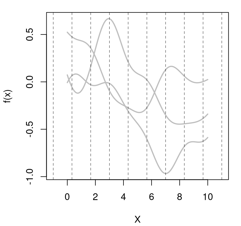
FIGURE 5.22: Three draws from a GP prior by convolution; knots \(\omega_j\) indicated by vertical dashed bars.
Generating from priors is fun, but learning from data is where real interest lies. When training data come along, possibly observed under noise, the generating mechanism above suggests the following model for the purposes of inference. Let
\[ y(x) = f(x) + \varepsilon, \quad \varepsilon \sim \mathcal{N}(0, \sigma^2), \]
which may be fit through an OLS regression, e.g.,
\[ Y_n = K_n \beta + \varepsilon, \quad \mbox{ where } \quad K_n^{ij} = k(x_i - \omega_j), \]
and \(x_i\) are training input \(x\)-values in the data, i.e., with \(x_i^\top\) filling out rows of \(X_n\). Whereas previously \(\beta\) was random, in the regression context their role changes to that of unknown parameter. Since that vector can be high dimensional, of length \(\ell\) for \(\ell\) knots, they’re usually inferred under some kind of regularization, i.e., ridge, lasso, full Bayes or through random effects. Notice that while \(K_n\) is potentially quite large (\(n \times \ell\)), if \(\ell\) is not too big we don’t need to decompose a big matrix. Consequently, such a variation could represent a substantial computational savings relative to canonical GP regression.
So the whole thing boils down to an ordinary linear regression, but instead of using the \(X_n\) inputs directly it uses features \(K_n\) derived from distances between \(x_i\) and \(\omega_j\)-values. By contrast, canonical GP regression entertains distances between all \(x_i\) and \(x_j\) in \(X_n\). This swap in distance anchoring set is similar in spirit to inducing point/pseudo input/predictive process approaches, reviewed in greater depth in Chapter 9. To see it in action, let’s return to the multi-tiered periodic example (5.19) from §5.3.4, originally from Higdon’s (2002) convolution GP paper.
First build training data quantities.
n <- length(x)
K <- as.data.frame(matrix(NA, ncol=ell, nrow=n))
for(j in 1:ell) K[,j] <- dnorm(x, omega[j])
names(K) <- paste0("omega", 1:ell)
Then fit the regression. For simplicity, OLS is entertained here without regularization. Since \(n\) is quite a bit bigger than \(\ell\) in this case, penalization to prevent numerical instabilities or high standard errors isn’t essential. Naming the columns of K helps when using predict below.
Notice that an intercept is omitted in the regression formula above: we’re assuming a zero-mean GP. Also it’s worth noting that the \(\hat{\sigma}^2\) estimated by lm is equivalent to \(\hat{\tau}^2 \hat{g}\) in our earlier, conventional GP specification.
Prediction on a grid in the input space at \(\mathcal{X} \equiv\) xx involves building out predictive feature space by evaluating the same kernel(s) at those new locations …
xx <- seq(-1, 11, length=100)
KK <- as.data.frame(matrix(NA, ncol=ell, nrow=length(xx)))
for(j in 1:ell) KK[,j] <- dnorm(xx, omega[j])
names(KK) <- paste0("omega", 1:ell)
… and then feeding those in as newdata into predict.lm. It’s essential that KK have the same column names as K.
Figure 5.23 shows the resulting predictive surface summarized as mean and 95% predictive interval(s).
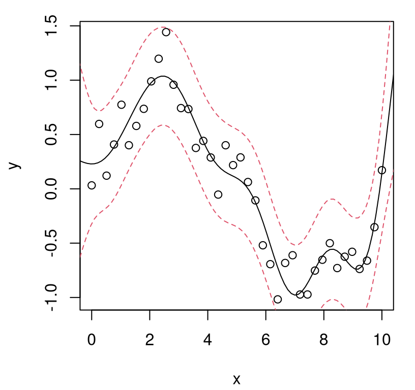
FIGURE 5.23: Posterior predictive under GP convolution.
That surface seems to agree with surfaces provided in Figure 5.21, which synthesized a grid of hyperparameter settings. Entertaining smaller lengthscales is a simple matter of providing a kernel with smaller variance. For example, the kernel below possesses an effective (square-root) lengthscale which is half the original, leading to a wigglier surface. See Figure 5.24.
for(j in 1:ell) K[,j] <- dnorm(x, omega[j], sd=0.5)
fit <- lm(y ~ . -1, data=K)
for(j in 1:ell) KK[,j] <- dnorm(xx, omega[j], sd=0.5)
p <- predict(fit, newdata=KK, interval="prediction")
plot(x, y)
lines(xx, p[,1])
lines(xx, p[,2], col=2, lty=2)
lines(xx, p[,3], col=2, lty=2)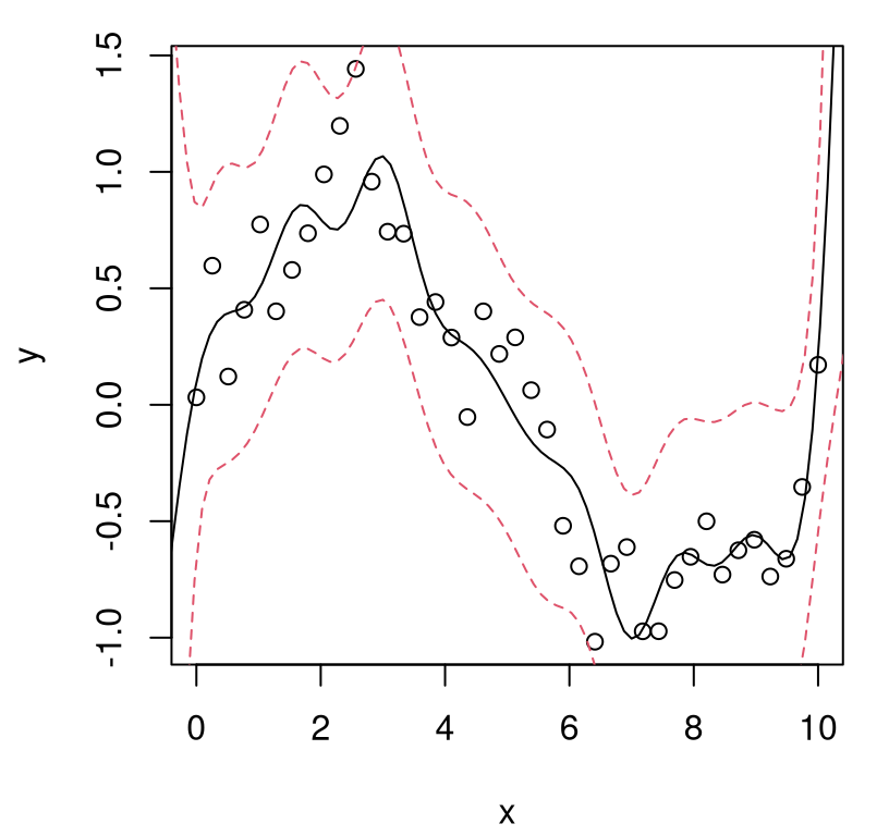
FIGURE 5.24: Predictive surface under a smaller kernel width/effective lengthscale; compare to Figure 5.23.
Fixing the number \(\ell\) and location of kernel centers, the \(\omega_j\)’s, and treating their common scale as unknown, inference can be performed with the usual suspects: likelihood (MLE or Bayes via least squares), CV, etc. Since this exposition is more of a side note, we’ll leave details to the literature. A great starting point is the Ph.D. dissertation of Chris Paciorek (2003), with references and links therein. One feature that this method accommodates rather more gracefully than a canonical GP approach involves relaxations of stationarity, which is the main methodological contribution in Chris’ thesis. Allowing kernels and their parameterization to evolve in space represents a computationally cheap and intuitive mechanism for allowing distance-based dynamics to vary geographically. The culmination of these ideas is packaged neatly by Paciorek and Schervish (2006). There has been a recent resurgence in this area with the advent of deep Gaussian processes (Dunlop et al. 2018; Damianou and Lawrence 2013).
One downside worth mentioning is the interplay between kernel width, determining effective lengthscale, and density of the \(\omega_j\)’s. For fixed kernel, accuracy of approximation improves as that density increases. For fixed \(\omega_j\), however, accuracy of approximation diminishes if kernel width becomes narrower (smaller variance in the Gaussian case) because that has the effect of increasing kernel-distance between \(\omega_j\)’s, and thus distances between them and inputs \(X_n\). Try the code immediately above with sd=0.1, for example. A kernel width of 0.1 may be otherwise ideal, but not with the coarse grid of \(\omega_j\)’s in place above; an order of magnitude denser grid (much bigger \(\ell\)) would be required. At the other end, larger kernel widths can be problematic numerically, leading to ill-conditioned Gram matrices \(K_n^\top K_n\) and thus problematic decompositions when solving for \(\hat{\beta}\). This can happen even when the column dimension \(\ell\) is small relative to \(n\).
Schemes allowing scale and density of kernels to be learned simultaneously, and which support larger effective lengthscales (even with fixed kernel density), require regularization and consequently demand greater computation as matrices K and KK become large and numerically unwieldy. Some kind of penalty on complexity, or shrinkage prior on \(\beta\), is needed to guarantee a well-posed least-squares regression problem and to prevent over-fitting, as can happen in any setting where bases can be expanded to fit noise at the expense of signal. This issue is exacerbated as input dimension increases. Bigger input spaces lead to exponentially increasing inter-point distances, necessitating many more \(\omega_j\)’s to fill out the void. The result can be exponentially greater computation and potential to waste those valuable resources over-fitting.
Speaking of higher input dimension, how do we do that? As long as you can fill out the input space with \(\omega_j\)’s, and increase the dimension of the kernel, the steps are unchanged. Consider a look back at our 2d data from earlier, which we conveniently saved as X2 and y2, in §5.2.4.
An \(\ell = 10 \times 10\) dense grid of \(\omega_j\)’s would be quite big – bigger than the data size \(n = 80\), comprised of two replicates of forty, necessitating regularization. We can be more thrifty by taking a page out of the space-filling design literature, using LHSs for knots \(\omega_j\)’s in just the same way we did for design \(X_n\). R code below chooses \(\ell = 20\) maximin LHS (§4.3) locations to ensure that \(\omega_j\)’s are as spread out as possible.
ell <- 20
omega <- maximinLHS(ell, 2)
omega[,1] <- (omega[,1] - 0.5)*6 + 1
omega[,2] <- (omega[,2] - 0.5)*6 + 1
Next build the necessary training data quantities. Rather than bother with a library implementing bivariate Gaussians for the kernel in 2d, code below simply multiplies two univariate Gaussian densities together. Since the two Gaussians have the same parameterization, this treatment is isotropic in the canonical covariance-based GP representation.
n <- nrow(X2)
K <- as.data.frame(matrix(NA, ncol=ell, nrow=n))
for(j in 1:ell)
  K[,j] <- dnorm(X2[,1], omega[j,1])*dnorm(X2[,2], omega[j,2])
names(K) <- paste0("omega", 1:ell)
Kernel-based features in hand, fitting is identical to our previous 1d example.
Now for predictive quantities on testing inputs. Code below re-generates predictive \(\mathcal{X} =\) XX values on a dense grid to ease visualization. Otherwise this development mirrors our build of training data features above.
xx <- seq(-2, 4, length=gn)
XX <- expand.grid(xx, xx)
KK <- as.data.frame(matrix(NA, ncol=ell, nrow=nrow(XX)))
for(j in 1:ell)
  KK[,j] <- dnorm(XX[,1], omega[j,1])*dnorm(XX[,2], omega[j,2])
names(KK) <- paste0("omega", 1:ell)
Since it’s easier to show predictive standard deviation than error-bars in this 2d context, the code below provides se.fit rather than interval="prediction" to predict.lm.
Figure 5.25 shows mean (left) and standard deviation (right) surfaces side-by-side. Training data inputs are indicated as open circles, and \(\omega_j\)’s as filled circles.
par(mfrow=c(1,2))
image(xx, xx, matrix(p$fit, ncol=gn), col=cols, main="mean",
  xlab="x1", ylab="x2")
points(X2)
points(omega, pch=20)
image(xx, xx, matrix(p$se.fit, ncol=gn), col=cols, main="sd",
  xlab="x1", ylab="x2")
points(X2)
points(omega, pch=20)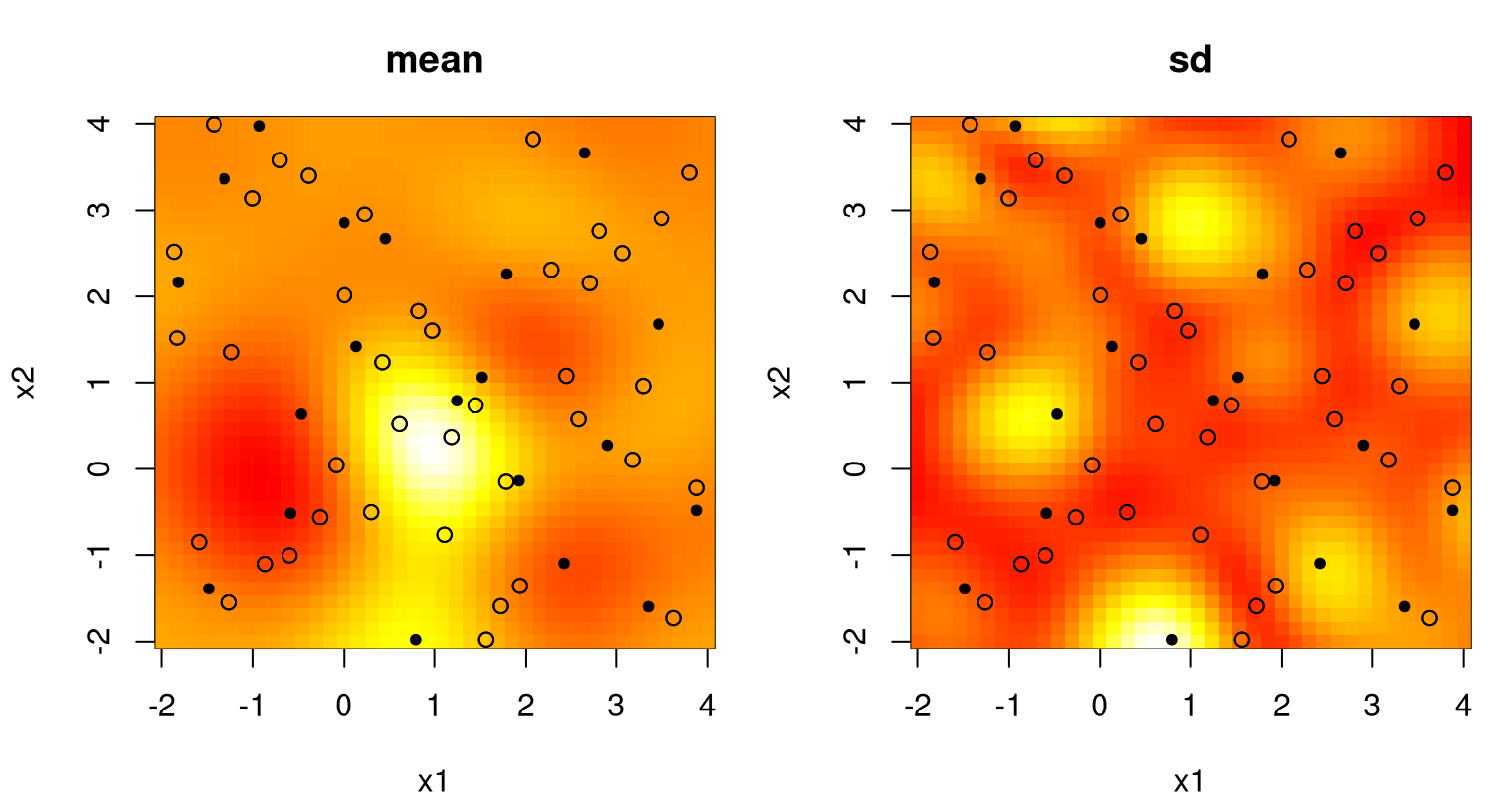
FIGURE 5.25: Convolution GP posterior predictive via mean (left) and standard deviation (right); compare with Figure 5.11. Design is indicated with open circles; knots as filled dots.
For my money, this doesn’t look as good as our earlier results in Figure 5.11. The signal isn’t as clear in either plot. Several explanations suggest themselves upon reflection. One is differing implicit lengthscale, in particular the one used immediately above is not fit from data. Another has to do with locations of the \(\omega_j\), and their multitude: \(\ell = 20\). Notice how both mean and sd surfaces exhibit “artifacts” near some of the \(\omega_j\). Contrasts are most stark in the sd surface, with uncertainty being much higher nearby filled circles which are far from open ones, rather than resembling sausages as seen earlier. Such behavior diminishes with larger \(\ell\) and when learning kernel widths from data, but at the expense of other computational and fitting challenges.
In two dimensions or higher, there’s potential for added flexibility by parameterizing the full covariance structure of kernels: tuning \(\mathcal{O}(m^2)\) unknowns in an \(m\)-dimensional input space, rather than forcing a diagonal structure with all inputs sharing a common width/effective lengthscale, yielding isotropy. A separable structure is a first natural extension, allowing each coordinate to have its own width. Rotations, and input-dependent scale (i.e., as a function of the \(\omega_j\)) is possible too, implementing a highly flexible nonstationary capability if a sensible strategy can be devised to infer all unknowns.
The ability to specify a flexible kernel structure that can warp in the input domain (expand, contract, rotate) as inferred by the data is seductive. That was Higdon’s motivation in his original 2001 paper, and the main subject of Paciorek’s thesis. But details and variations, challenges and potential solutions, are numerous enough in today’s literature (e.g., Dunlop et al. 2018), almost twenty years later, to fill out a textbook of their own. Unfortunately, those methods extend poorly to higher dimension because of the big \(\ell\) required to fill out an \(m\)-dimensional space, usually \(\ell \propto 10^m\) with \(\mathcal{O}(\ell^3)\) computation. Why is this a shame? Because it’s clearly desirable to have some nonstationary capability, which is perhaps the biggest drawback of the canonical (stationary) GP regression setup, as demonstrated below.
5.4.2 Limits of stationarity
If \(\Sigma(x, x') \equiv k(x - x')\), which is what it means for a spatial process to be stationary, then covariance is measured the same everywhere. That means we won’t be able to capture dynamics whose nature evolves in the input space, like in our motivating NASA LGBB example (§2.1). Recall how dynamics in lift exhibit an abrupt change across the sound barrier. That boundary separates a “turbulent” lift regime for high angles of attack from a relatively flat relationship at higher speeds. Other responses show tame dynamics away from mach 1, but interesting behavior nearby.
Taking a global view of the three-dimensional input space, LGBB lift exhibits characteristically nonstationary behavior. Locally, however, stationary dynamics reign except perhaps right along the mach 1 boundary, which may harbor discontinuity. How can we handle data of this kind? One approach is to ignore the problem: fit an ordinary stationary GP and hope for the best. As you might guess, ordinary GP prediction doesn’t fail spectacularly because good nonparametric methods have a certain robustness about them, as demonstrated in several variations in this chapter. But that doesn’t mean there isn’t room for improvement.
As a simpler illustration, consider the following variation on the multi-scale periodic process from §5.3.4.
X <- seq(0,20,length=100)
y <- (sin(pi*X/5) + 0.2*cos(4*pi*X/5)) * (X <= 9.6)
lin <- X>9.6
y[lin] <- -1 + X[lin]/10
y <- y + rnorm(length(y), sd=0.1)
The response is wiggly, identical to (5.19) from Higdon (2002) to the left of \(x=9.6\), and straight (linear) to the right. This example was introduced by Gramacy and Lee (2008a) as a cartoon mimicking LGBB behavior (§2.1) in a toy 1d setting. Our running 2d example from §5.1.2 was conceived as a higher-dimensional variation. To keep the discussion simpler here, we’ll stick to 1d and return to the others in Chapter 9.
Consider the following stationary GP fit to these data using methods from laGP.
Above, isotropic routines are used rather than separable ones. It makes no difference in 1d. As an aside, we remark that the jmleGP function is similar to mleGPsep with argument param="both"; “j” here is for “joint”, meaning both lengthscale and nugget. Rather than using a gradient over both parameters, as mleGPsep does, jmleGP performs a coordinate-wise, or profile-style, maximization iterating until convergence for one hyperparameter conditional on the other, etc. Sometimes this approach leads to more numerically stable behavior; jmleGPsep works similarly for separable Gaussian kernels.
Once hyperparameters have been estimated, prediction proceeds as usual.
Now we’re ready to visualize the fit, as provided by predictive mean and 95% intervals in Figure 5.26.
plot(X, y, xlab="x")
lines(X, p$mean)
lines(X, p$mean + 2*sqrt(p$s2), col=2, lty=2)
lines(X, p$mean - 2*sqrt(p$s2), col=2, lty=2)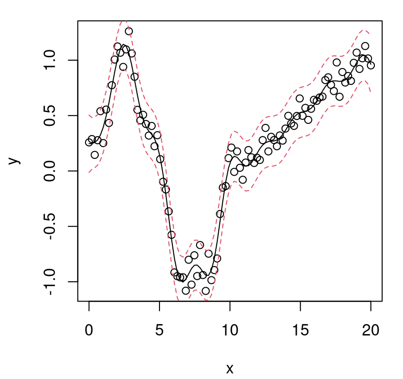
FIGURE 5.26: GP fit to an inherently nonstationary input–output relationship.
Observe how the predictive equations struggle to match disparate behavior in the two regimes. Since only one lengthscale must accommodate the entire input domain, the likelihood is faced with a choice between regimes and in this case it clearly favors the left-hand one. A wiggly fit to the right-hand regime is far better than a straight fit to left. As a result, wiggliness bleeds from the left to right.
Two separate GP fits would have worked much better. Consider …
left <- X < 9.6
gpl <- newGP(matrix(X[left], ncol=1), y[left], d=0.1,
  g=0.1*var(y), dK=TRUE)
mlel <- jmleGP(gpl)
gpr <- newGP(matrix(X[!left], ncol=1), y[!left], d=0.1,
  g=0.1*var(y), dK=TRUE)
mler <- jmleGP(gpr, drange=c(eps, 100))
To allow the GP to acknowledge a super “flat” right-hand region, the lengthscale (d) range has been extended compared to the usual default. Notice how this approximates a (more) linear fit; alternatively – or perhaps more parsimoniously – a simple lm command could be used here instead.
Now predicting …
pl <- predGP(gpl, matrix(X[left], ncol=1), lite=TRUE)
deleteGP(gpl)
pr <- predGP(gpr, matrix(X[!left], ncol=1), lite=TRUE)
deleteGP(gpr)
… and finally visualization in Figure 5.27.
plot(X, y, xlab="x")
lines(X[left], pl$mean)
lines(X[left], pl$mean + 2*sqrt(pl$s2), col=2, lty=2)
lines(X[left], pl$mean - 2*sqrt(pl$s2), col=2, lty=2)
lines(X[!left], pr$mean)
lines(X[!left], pr$mean + 2*sqrt(pr$s2), col=2, lty=2)
lines(X[!left], pr$mean - 2*sqrt(pr$s2), col=2, lty=2)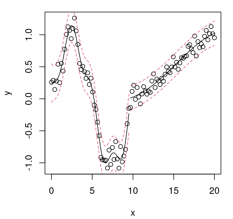
FIGURE 5.27: Partitioned GP fit to a nonstationary input–output relationship. Compare to Figure 5.26.
Aesthetically this is a much better fit. Partitioning can be a powerful tool for flexible modeling, and not just for GPs. Divide-and-conquer can facilitate nonstationarity, through spatial statistical independence, and yield faster calculations with smaller datasets and much smaller \(\mathcal{O}(n^3)\) matrix decompositions. The two fits can even be performed in parallel.
But how to know where to partition without knowing the data generating mechanism? It turns out that there are several clever solutions to that problem. Read on in Chapter 9. In the meantime, we shall see going forward that even stationary GPs have many interesting applications and success stories – as response surfaces, for optimization, calibration and input sensitivity analysis, and more – without worrying (much) about how ideal fits are.
5.4.3 Functional and other outputs
Focus has been on \(Y(x) \in \mathbb{R}\); i.e., surrogate modeling for scalar, real-valued outputs. That will remain so throughout the text, but it’s worthwhile commenting on what’s available in greater generality. Modeling a small handful of real-valued outputs simultaneously is easy and hard at the same time. It’s easy because treating each scalar output independently works surprisingly well. Gramacy and Lee (2009) modeled six LGBB outputs (§2.1) independently and without any perceivable ill-effect. It’s hard because just about anything else you try can both be unwieldy and underwhelming. Effective, general-purpose multi-output surrogate modeling lies on the methodological frontier, as it were.
If there’s a small number \(p\) of outputs following the same underlying spatial field, but experiencing correlated random shocks of varying magnitude, then cokriging (Ver Hoef and Barry 1998) could help. The idea is to combine \(p \times p\) covariances \(\Sigma^{(Y)}_p\) with the usual \(n\times n\) inverse distance-based ones \(\Sigma_n = \tau^2 (K_n + \mathbb{I} _n g)\) in a Kronecker layout. Inference for \(\Sigma^{(Y)}_n\) is relatively straightforward. MLE and Bayesian posterior are available in closed form conditional on \(\Sigma_n\). Trouble is, this isn’t a very realistic situation, at least not when data are generated through computer simulation. One exception may be when outputs differ from one another only in resolution or fidelity of simulations. Cokriging has been applied with some success in such multifidelity settings (Le Gratiet and Garnier 2014; Le Gratiet and Cannamela 2015).
The linear model of coregionalization [LMC; Journel and Huijbregts (1978); Goovaerts (1997)] is a special case or generalization of cokriging depending upon your perspective. Sometimes cokriging, as described above, is referred to an intrinsic coregionalization model (ICM). As the name suggests, LMC allows for a more flexible, linear and covarying relationship between outputs. LMC’s most prominent success stories in computer surrogate modeling involve simulators providing additional derivative information. Taylor’s theorem justifies a linear structure. For examples, see Bompard, Peter, and Desideri (2010) and references therein. For a machine learning perspective and Python implementation, see GPy.
Functional output is rather more common in our field. Simulators may provide realizations \(Y(x,t) \in \mathbb{R}\) across an entire index set \(t=1,\dots,T\), simultaneously for each \(x\). I’ve chosen \(t\) to represent output indices because functions of time are common. Two-dimensional indexing for image data is also typical. Theoretically, such processes are easy to model with GP surrogates as long as indices are naturally ordered, or otherwise emit a reasonable set of pairwise distances so that off-the-shelf covariance kernels apply. In other words, treating the output index \(t\) as another set of input coordinates is an option. Some have taken to calling this a “left to right mapping”: moving output indices from the left side of the (probability) conditioning bar to the right. A similar tack may be taken with small-\(p\) outputs (previous paragraph) as long as an appropriate kernel for mixed quantitative and qualitative inputs can be found (Qian, Wu, and Wu 2008; Y. Zhang et al. 2018). The trouble is, this idea is hard to put into practice if \(N = n \times T\) is big, as it would be with any nontrivial \(T\). Working with \(N \times N\) matrices becomes unwieldy except by approximation (Chapter 9), or when the design in \(x\)-space has special structure (e.g., high degrees of replication, as in Chapter 10).4
A more parsimonious approach leverages functional bases for outputs and independent surrogate modeling of weights corresponding to a small number of principal components of that basis (Higdon et al. 2008). This idea was originally developed in a calibration setting (§8.1), but has gained wide traction in a number of surrogate modeling situations. MATLAB software is available as part of the GPMSA toolkit (Gattiker et al. 2016). Fadikar et al. (2018) demonstrate use in a quantile regression setting (Plumlee and Tuo 2014) for an epidemiological inverse problem pairing a disease outbreak simulator to Ebola data from Liberia. Sun, Gramacy, Haaland, Lu, et al. (2019) describe a periodic basis for GP smoothing of hourly simulations of solar irradiance across the continental USA. A cool movie showing surrogate irradiance predictions over the span of a year can be found here.
Finally, how about categorical \(Y(x)\)? This is less common in the computer surrogate modeling literature, but GP classification remains popular in ML. See Chapter 3 of Rasmussen and Williams (2006). Software is widely available in Python (e.g., GPy) and MATLAB/Octave (see gpstuff Vanhatalo et al. (2012)). R implementation is provided in kernlab (Karatzoglou, Smola, and Hornik 2018) and plgp (Gramacy 2014). Bayesian optimization under constraints (§7.3) sometimes leverages classification surrogates to model binary constraints. GP classifiers work well here (Gramacy and Lee 2011), but so too do other common nonparametric classifiers like random forests (Breiman 2001). See §7.3.2 for details.
5.5 Homework exercises
These exercises give the reader an opportunity to explore Gaussian process regression, properties, enhancements and extensions, and related methods.
#1: Bayesian zero-mean GP
Consider the following data-generating mechanism \(Y \sim \mathcal{N}_n (0, \tau^2 K_n)\) and place prior \(\tau^2 \sim \mathrm{IG}\left(\frac{a}{2}, \frac{b}{2}\right)\) on the scale parameter. Use the following parameterization of inverse gamma \(\mathrm{IG}(\theta; \alpha, \beta)\) density, expressed generically for a parameter \(\theta > 0\) given shape \(\alpha > 0\) and scale \(\beta > 0\): \(f(\theta) = \frac{\beta^\alpha}{\Gamma(\alpha)} \theta^{-(\alpha+1)} e^{-\beta/\theta}\), where \(\Gamma\) is the gamma function.
- Show that the IG prior for \(\tau^2\) is conditionally conjugate by deriving the closed form of the posterior conditional distribution for \(\tau^2\) given all other hyperparameters, i.e., those involved in \(K_n\).
- Choosing \(a = b = 0\) prescribes a reference prior (Berger, De Oliveira, and Sansó 2001; Berger, Bernardo, and Sun 2009) which is equivalent to \(p(\tau^2) \propto 1/\tau^2\). This prior is improper. Nevertheless, derive the closed form of the posterior conditional distribution for \(\tau^2\) and argue that it’s proper under a condition that you shall specify. Characterize the posterior conditional for \(\tau^2\) in terms of \(\hat{\tau}^2\).
- Now consider inference for the hyperparameterization of \(K_n\). Derive the marginal posterior \(p(K_n \mid Y_n)\), i.e., as may be obtained by integrating out the scale parameter \(\tau^2\) under the IG prior above; however, you may find other means equally viable. Use generic \(p(K_n)\) notation for the prior on covariance hyperparameterization, independent of \(\tau^2\). How does this (log) posterior density compare to the concentrated log likelihood (5.8) under the reference prior?
- Deduce the form of the marginal predictive equations \(p(Y(x) \mid K_n, Y_n)\) at a new location \(x\), i.e., as may be obtained by integrating out \(\tau^2\). Careful, they’re not Gaussian but they’re a member of a familiar family. How do these equations change in the reference prior setting?
#2: GP with a linear mean
Consider the following data-generating mechanism \(Y \sim \mathcal{N}_n (\beta_0 + X_n\beta, \tau^2 K_n)\) where
- \(K_n = C_n + g \mathbb{I}_n\),
- \(C_n\) is an \(n \times n\) correlation matrix defined by a positive definite function \(C_\theta(x, x')\) calculated on the \(n\) rows of \(X_n\), and which has lengthscale hyperparameters \(\theta\),
- and \(g\) is a nugget hyperparameter, which must be positive.
There are no restrictions on the coefficients \(\beta_0\) and \(\beta\), except that the dimension \(m\) of \(\beta\) matches the column dimension of \(X_n\).
- Argue, at a high level, that this specification is essentially equivalent to the following semiparametric model \(y(x) = \beta_0 + x^\top \beta + w(x) + \varepsilon\), and describe what each component means, and/or what distribution it’s assumed to have.
- Conditional on hyperparameters \(\theta\) and \(g\), obtain closed form expressions for the MLE \(\hat{\tau}^2\), \(\hat{\beta}_0\) and \(\hat{\beta}\). You might find it convenient to assume, for the purposes of these calculations, that \(X_n\) contains a leading column of ones, and that \(\beta \equiv [\beta_0, \beta]\).
- Provide a concentrated (log) likelihood expression \(\ell(\theta,g)\) that plugs-in expressions for \(\hat{\tau}^2\), \(\hat{\beta}_0\) and \(\hat{\beta}\) (or a combined \(\hat{\beta}\)) which you derived above.
- Using point estimates for \(\hat{\beta}\), \(\hat{\tau}^2\) and conditioning on \(\theta\) and \(g\) settings, derive the predictive equations.
#3: Bayesian linear-mean GP
Complete the setup in #2 above with prior \(p(\beta, \tau^2) = p(\beta \mid \tau^2)p(\tau^2)\) where \(\beta\mid \tau^2 \sim \mathcal{N}_{m+1}(B, \tau^2 V)\) and \(\tau^2 \sim \mathrm{IG}\left(\frac{a}{2}, \frac{b}{2}\right)\). Notice that the intercept term \(\beta_0\) is subsumed into \(\beta\) in this notation.
- Show that the MVN prior for \(\beta \mid \tau^2\) is conditionally conjugate by deriving the closed form of the posterior conditional distribution for \(\beta \mid \tau^2, Y_n\) and given all other hyperparameters, i.e., those involved in \(K_n\).
- Show that the IG prior for \(\tau^2\) is conditionally conjugate by deriving the closed form of the posterior conditional distribution for \(\tau^2 \mid \beta, Y_n\) and given all other hyperparameters, i.e., those involved in \(K_n\).
- Under the reference prior \(p(\beta, \tau^2) \propto 1/\tau^2\), which is improper, how do the forms of the posterior conditionals change? Under what condition(s) are these conditionals still proper? (Careful, proper conditionals don’t guarantee a proper joint.) Express the \(\beta\) conditional as function of \(\hat{\beta}\) from exercise #2.
For the remainder of this question, parts #d–f, use the reference prior to keep the math simple.
- Derive the marginalized posterior distribution \(\tau^2 \mid Y_n\) and given \(K_n\), i.e., as may be obtained by integrating out \(\beta\), however you may choose to utilize other means. Express your distribution as a function of \(\hat{\beta}\) and \(\hat{\tau}^2\) from exercise #2.
- Now consider inference for the hyperparameterization of \(K_n\). Derive the marginal posterior \(p(K_n \mid Y_n)\) up to a normalizing constant, i.e., as may be obtained by integrating out both linear mean parameter \(\beta\) and scale \(\tau^2\) under their joint reference prior. Use generic \(p(K_n)\) notation for the prior on covariance hyperparameterization, independent of \(\tau^2\) and \(\beta\). How does the form of this density compare to the concentrated log likelihood in #2c above? Under what condition(s) is this density proper?
- Deduce the form of the marginal predictive equations \(p(Y(x) \mid K_n, Y_n)\) at a new location \(x\), i.e., as may be obtained by integrating out \(\beta\) and \(\tau^2\). Careful, they’re not Gaussian but they’re a member of a familiar family.
#4: Implementing the Bayesian linear-mean GP
Code up the marginal posterior \(p(K_n \mid Y_n)\) from #3e and the marginal predictive equations \(p(Y(x) \mid K_n, Y_n)\) from #3f and try them out on the Friedman data. Take the reference prior \(p(\beta, \tau^2) \propto 1/\tau^2\) and define \(p(K_n)\) as independent gamma priors on isotropic (Gaussian family) lengthscale and nugget as follows:
\[ \theta \sim G(3/2, 1) \quad \mbox{ and } \quad g \sim G(3/2, 1/2), \]
providing shape and rate parameters to dgamma in R, respectively.
- Use the marginal posterior as the basis of a Metropolis–Hastings scheme for sampling from the posterior distribution of lengthscale \(\theta\) and nugget \(g\) hyperparameters. Provide a visual comparison between these marginal posterior densities and the point estimates we obtained in the chapter. How influential was the prior?
- Use the marginal posterior predictive equations to augment Table 5.1’s RMSEs and scores collecting out-of-sample results from comparators in §5.2.5–5.2.6. (You might consider more random training/testing partitions as in our bakeoff in §5.2.7, extended in #7 below.)
- Use boxplots to summarize the marginal posterior distribution of regression coefficients \(\beta\). Given what you know about the Friedman data generating mechanism, how do these boxplots compare with the “truth”? You will need #3d and #3a for this part.
Suppose you knew, a priori, that only the first three inputs contributed nonlinearly to response. How would you change your implementation to reflect this knowledge, and how do the outputs/conclusions (#ii–iii) change?
#5: Matérn kernel
Revisit noise-free versions of our 1d sinusoidal (§5.1.1 and Figure 5.3) and 2d exponential (§5.1.2 and Figure 5.5) examples with Matérn \(\nu = 3/2\) and \(\nu = 5/2\) kernels (5.18). Extend concentrated log likelihood and gradient functions to learn an \(m\)-vector of lengthscale hyperparameters \(\hat{\theta}\) using nugget \(g=0\) and no \(\epsilon\) jitter. Define this separable Matérn in product form as \(k_{\nu,\theta}(r) = \prod_{\ell=1}^m k_{\nu, \theta_\ell}(r^{(\ell)})\) where \(r^{(\ell)}\) is based on (original, not squared) distances calculated only on the \(\ell^{\mathrm{th}}\) input coordinate. Provide visuals of the resulting surfaces using the predictive grids established along with those examples. Qualitatively (looking at the visuals) and quantitatively (via Mahalanobis distance (5.7) calculated out of sample), how do these surfaces compare to the Gaussian kernel alternative (with jitter and with estimated lengthscale(s))?
For another sensible vectorized lengthscale option, see “ARD Matérn” here. ARD stands for “automatic relevance determination”, which comes from the neural networks/machine learning literature, allowing a hyperparameter to control the relative relevance of each input coordinate. For the Gaussian family the two definitions, product form and ARD, are the same. But for Matérn they differ ever-so-slightly.
#6: Splines v. GP
Revisit the 2d exponential data (§5.1.2 and Figure 5.5), and make a comparison between spline and GP predictors. For a review of splines, see the supplement linked here. Generate a random uniform design of size \(n=100\) in \([-2,4]^2\) and observe random responses under additive Gaussian error with a mean of zero and a standard deviation of 0.001. This is your training set. Then generate a dense \(100 \times 100\) predictive grid in 2d, and obtain (again noisy) responses at those locations, which you will use as a testing set.
Ignoring the testing responses, use the training set to obtain predictions on the testing input grid under
- a spline model with a tensor product basis provided in splines2d.R;
- a zero-mean GP predictor with an isotropic Gaussian correlation function, whose hyperparameters (including nugget, scale, and lengthscale) are inferred by maximum likelihood;
- MARS in the
mdapackage for R.
You may wish to follow the format in splines2d.R for your GP and MARS comparators. Consider the following benchmarking metrics:
- computation time for inference and prediction combined;
- RMSE on the testing set.
Once you’re satisfied with your setup using one random training/testing partition, put a “for” loop around everything and do 99 more MC repetitions of the experiment (for 100 total), each with novel random training and testing set as defined above. Make boxplots collecting results for #i–ii above and thereby summarize the distribution of those metrics over the randomized element(s) in the experiment.
#7: MARS v. GP redux
Revisit the MARS v. GP bakeoff (§5.2.7) with five additional predictors.
- MARS via
mdawithdegree=2. - MARS via
earthwith default arguments. - MARS via
earthwithdegree=2. - Bayesian MARS via the
bassfunction with default arguments from theBASSpackage (Francom 2017) on CRAN. - Bayesian GP with jumps to the limiting linear model [LLM; Gramacy and Lee (2008b)] via
bgpllmwith default arguments in thetgppackage on CRAN.
Rebuild the RMSE and time boxplots to incorporate these new predictors; ignore proper score unless you’d like to comb tgp and BASS documentation to figure out how to extract predictive covariance matrices, which are not the default.
BASS supports a simulated tempering scheme to avoid Markov chains becoming stuck in local modes of the posterior. Devin Francom recommends the following call for best results on this exercise.
fit.bass <- bass(X, y, verbose=FALSE, nmcmc=40000, nburn=30000, thin=10,
  temp.ladder=(1+0.27)^((1:9)-1))
A similar importance tempering feature (Gramacy, Samworth, and King 2010) is implemented in tgp and is described in more detail in the second package vignette (Gramacy and Taddy 2010). Also see ?default.itemps in the package documentation. The curious reader may wish to incorporate these gold standards for brownie points.
#8: Langley Glide-Back Booster
In this problem, revisit #6 on the “original” LGBB drag response.
However note that the scales of LGBB’s inputs are heterogeneous, and quite different from #6. In the least, it’d be wise to code your inputs. For best results, you might wish to upgrade the isotropic GP comparator from #6 to a separable version.
- Consider the subset of the data where the side-slip angle is zero, so that it’s a 2d problem. Create a random training and testing partition in the data so that about half are for training and half for testing, and then perform exactly #a–c with #i–ii from #6, above, and report on what you find.
- Put a “for” loop around everything and do 100 MC repetitions of the above experiment, each with novel random training and testing set as defined above. Then, make boxplots for RMSE results collected for #i–ii above and thereby summarize the distribution of those metrics over randomized element(s) in the experiment.
- Now return to the full set of data, i.e., for all side-slip angles. Since the number of observations, \(n\), is bigger than 3000, you won’t be able to get very far with a random 50:50 split. Instead, do a 20:80 split or whatever you think you can manage. Also, it’ll be tough to do a spline approach with a tensor product basis in 3d, so perhaps ignore comparator #6a unless you’re feeling particularly brave. Otherwise perform exactly #a–c with #i–ii from #6, above, and report on what you find. (That is, do like in part #A, without the “for” loop in #B.)
- Repeat #C with a GP scheme using an axis-aligned partition. Fit two GP models in 3d where the first one uses the subset of the training data with
mach < 2and the second usesmach >= 2. Since you’re dividing-and-conquering, you can probably afford a 50:50 split for training and testing.
#9: Convolution kernel width
Revisit the 1d multi-tiered periodic example (5.19) as treated by convolution in §5.4.1.
- Write down a concentrated log likelihood for the kernel width parameter \(\theta\), notated as
sdin the example, and provide an implementation in code. - Plot the concentrated log likelihood over the range
sd\(\equiv \theta \in [0.4, 4]\) and note the optimal setting. - Verify the result with
optimizeon your concentrated log likelihood. - How does the value you inferred compare to the two settings entertained in §5.4.1? How do the three predictive surfaces compare visually?
References
mlegp: Maximum Likelihood Estimates of Gaussian Processes. https://CRAN.R-project.org/package=mlegp.
kergp: Gaussian Process Laboratory. https://CRAN.R-project.org/package=kergp.
spBayes: Univariate and Multivariate Spatial-Temporal Modeling. https://CRAN.R-project.org/package=spBayes.
mvtnorm: Multivariate Normal and \(t\) Distributions. https://CRAN.R-project.org/package=mvtnorm.
plgp: Particle Learning of Gaussian Processes. https://CRAN.R-project.org/package=plgp.
laGP: Large-Scale Spatial Modeling via Local Approximate Gaussian Processes in R.” Journal of Statistical Software 72 (1): 1–46.
laGP: Local Approximate Gaussian Process Regression. http://bobby.gramacy.com/r_packages/laGP.
tgp Version 2, an R Package for Treed Gaussian Process Models.” Journal of Statistical Software 33 (6): 1–48.
tgp: Bayesian Treed Gaussian Process Models. https://CRAN.R-project.org/package=tgp.
RobustGaSP: Robust Gaussian Stochastic Process Emulation. https://CRAN.R-project.org/package=RobustGaSP.
emulator: Bayesian Emulation of Computer Programs. https://CRAN.R-project.org/package=emulator.
kernlab: Kernel-Based Machine Learning Lab. https://CRAN.R-project.org/package=kernlab.
mda: Mixture and Flexible Discriminant Analysis. https://CRAN.R-project.org/package=mda.
GPfit: Gaussian Processes Modeling. https://CRAN.R-project.org/package=GPfit.
earth: Multivariate Adaptive Regression Splines. https://CRAN.R-project.org/package=earth.
fields: Tools for Spatial Data. https://CRAN.R-project.org/package=fields.
spatial: Functions for Kriging and Point Pattern Analysis. https://CRAN.R-project.org/package=spatial.