Chapter 10 Heteroskedasticity
Historically, design and analysis of computer experiments focused on deterministic solvers from the physical sciences via Gaussian process (GP) interpolation (Sacks et al. 1989). But nowadays computer modeling is common in the social (Cioffi–Revilla 2014, chap. 8), management (Law 2015) and biological (L. Johnson 2008) sciences, where stochastic simulations abound. Queueing systems and agent-based models replace finite elements and simple Monte Carlo (MC) with geometric convergence (Picheny and Ginsbourger 2013). Data in geostatistics (Banerjee, Carlin, and Gelfand 2004) and machine learning [ML; Rasmussen and Williams (2006)] aren’t only noisy but frequently involve signal-to-noise ratios that are low or changing over the input space. Noisier simulations/observations demand bigger experiments/studies to isolate signal from noise, and more sophisticated GP models – not just adding nuggets to smooth over noise, but variance processes to track changes in noise throughout the input space in the face of that heteroskedasticity.
Modeling methodology for large simulation efforts with intrinsic stochastic dynamics has lagged until recently. Partitioning is one option (§9.2.2), but leaves something to be desired when underlying processes are smooth and signal-to-noise ratios are low. A theme in this chapter is that replication, a tried and true design strategy for separating signal from noise, can play a crucial role in computationally efficient heteroskedastic modeling, especially with GPs. To be concrete, replication here means repeated \(y\)-observations at the same input \(x\) setting. In operations research, stochastic kriging [SK; Ankenman, Nelson, and Staum (2010)] offers approximate methods that exploit large degrees of replication. Its independent method of moments-based inferential framework can yield an efficient heteroskedastic modeling capability. However the setup exploited by SK is highly specialized; moment-based estimation can strain coherency in a likelihood dominated surrogate landscape. Here focus is on a heteroskedastic GP technology (Binois, Gramacy, and Ludkovski 2018) that offers a modern blend of SK and ideas from ML (largely predating SK: Goldberg, Williams, and Bishop 1998; Quadrianto et al. 2009; Boukouvalas and Cornford 2009; Lazaro–Gredilla and Titsias 2011).
Besides leveraging replication in design, the idea is: what’s good for the mean is good for the variance. If it’s sensible to model the latent (mean) field with GPs (§5.3.2), why not extend that to variance too? Unfortunately, latent variance fields aren’t as easy to integrate out. (Variances must also be positive, whereas means are less constrained.) Numerical schemes are required for variance latent learning, and there are myriad strategies – hence the plethora of ML citations above. Binois, Gramacy, and Ludkovski (2018)’s scheme remains within our familiar class of library-based (e.g., BFGS) likelihood-optimizing methodology, and is paired with tractable strategies for sequential design (Binois et al. 2019) and Bayesian optimization (BO; Chapter 8). Other approaches achieving a degree of input-dependent variance include quantile kriging [QK; Plumlee and Tuo (2014)]; use of pseudoinputs (Snelson and Ghahramani 2006) or predictive processes (Banerjee et al. 2008); and (non-GP-based) tree methods (M. Pratola et al. 2017). Unfortunately, none of those important methodological contributions, to my knowledge, pair with design, BO or open source software.
Illustrations here leverage hetGP (Binois and Gramacy 2019) on CRAN, supporting a wide class of alternatives in the space of coupled-GP heteroskedastic (and ordinary homoskedastic) modeling, design and optimization.
10.1 Replication and stochastic kriging
Replication can be a powerful device for separating signal from noise, offering a pure look at noise not obfuscated by signal. When modeling with GPs, replication in design can yield substantial computational savings as well. Continuing with \(N\)-notation from Chapter 9, consider training data pairs \((x_1, y_1), \dots, (x_N, y_N)\). These make up the “full-\(N\)” dataset \((X_N, Y_N)\). Now suppose that the number \(n\) of unique \(x_i\)-values in \(X_N\) is far smaller than \(N\), i.e., \(n \ll N\). Let \(\bar{Y}_n = (\bar{y}_1, \dots, \bar{y}_n)^\top\) collect averages of \(a_i\) replicates at unique locations \(\bar{x}_i\), and similarly let \(\hat{\sigma}^2_i\) collect normalized residual sums of squares for those replicate measurements:
\[ \bar{y}_i = \frac{1}{a_i} \sum_{j=1}^{a_i} y_i^{(j)} \quad \mbox{and} \quad \hat{\sigma}^2_i = \frac{1}{a_i - 1} \sum_{j=1}^{a_i} (y_i^{(j)} - \bar{y}_i)^2. \]
Unfortunately, \(\bar{Y}_n = (\bar{y}_1, \dots, \bar{y}_n)^\top\) and \(\hat{\sigma}_{1:n}^2\) don’t comprise of a set of sufficient statistics for GP prediction under the full-\(N\) training data. But these are nearly sufficient: only one quantity is missing and will be provided momentarily in §10.1.1. Nevertheless “unique-\(n\)” predictive equations based on \((\bar{X}_n, \bar{Y}_n)\) are a best linear unbiased predictor (BLUP):
\[\begin{align} \mu^{\mathrm{SK}}_n(x) &= \nu k_n^\top(x) (\nu C_n + S_n)^{-1} \bar{Y}_n \notag \\ \sigma^{\mathrm{SK}}_n(x)^2 &= \nu K_\theta(x,x) - \nu^2 k_n^\top(x) (\nu C_n + S_n)^{-1} k_n(x), \tag{10.1} \end{align}\]
where \(k_n(x) = (K_\theta(x, \bar{x}_1), \dots, K_\theta(x, \bar{x}_n))^\top\) as in Chapter 5,
\[ S_n = [\hat{\sigma}_{1:n}^2] A_n^{-1} = \mathrm{Diag}(\hat{\sigma}_1^2/a_1, \dots, \hat{\sigma}_n^2/a_n), \]
\(C_n = \{ K_\theta(\bar{x}_i, \bar{x}_j)\}_{1 \leq i, j \leq n}\), and \(a_i \gg 1\). This is the basis of stochastic kriging [SK; Ankenman, Nelson, and Staum (2010)], implemented as an option in DiceKriging (Roustant, Ginsbourger, and Deville 2018) and mlegp (Dancik 2018) packages on CRAN. SK’s simplicity is a virtue. Notice that when \(n = N\), all \(a_i = 1\) and \(\hat{\sigma}_i^2 = \nu g\), a standard GP predictor (§5) is recovered when mapping \(\nu = \tau^2\).10 Eq. (10.1) has intuitive appeal as an application of ordinary kriging equations (5.2) on (almost) sufficient statistics. An independent moments-based estimate of variance is used in lieu of the more traditional, likelihood-based (hyperparametric) alternative. This could be advantageous if variance is changing in the input space, as discussed further in §10.2. Computational expedience is readily apparent even in the usual homoskedastic setting: \(S_n = \mathrm{Diag}(\frac{1}{n} \sum \hat{\sigma}_i^2)\). Only \(\mathcal{O}(n^3)\) matrix decompositions are required, which could represent a huge savings compared with \(\mathcal{O}(N^3)\) if the degree of replication is high.
Yet independent calculations have their drawbacks. Thinking heteroskedastically, this setup lacks a mechanism for specifying a belief that variance evolves smoothly over the input space. Lack of smoothness thwarts a pooling of variance that’s essential for predicting uncertainties out-of-sample at novel \(x' \in \mathcal{X}\). Basically we don’t know \(K_\theta(x, x)\) in Eq. (10.1), whereas homoskedastic settings use \(1+g\) for all \(x\). Ankenman, Nelson, and Staum (2010) suggest smoothing \(\hat{\sigma}_i^2\)-values with a second GP, but that two-stage approach will feel ad hoc compared to what’s presented momentarily in §10.2. More fundamentally, numbers of replicates \(a_i\) must be relatively large in order for the \(\hat{\sigma}^2_i\)-values to be reliable. Ankenman et al. recommend \(a_i \geq 10\) for all \(i\), which can be prohibitive. Thinking homoskedastically, the problem with this setup is that it doesn’t emit a likelihood for inference for other hyperparameters, such as lengthscale(s) \(\theta\) and scale \(\nu\). Again, this is because \((\bar{Y}_n, S_n)\) don’t quite constitute a set of sufficient statistics for hyperparameter inference.
10.1.1 Woodbury trick
The fix, ultimately revealing the full set of sufficient statistics for prediction and likelihood-based inference, involves Woodbury linear algebra identities. These are not unfamiliar to the spatial modeling community (e.g., Opsomer et al. 1999; Banerjee et al. 2008; Ng and Yin 2012). However, their application toward efficient GP inference under replicated design is relatively recent (Binois, Gramacy, and Ludkovski 2018). Let \(D\) and \(B\) be invertible matrices of size \(N \times N\) and \(n \times n\), respectively, and let \(U\) and \(V^\top\) be matrices of size \(N\times n\). The Woodbury identities are
\[\begin{align} (D + UBV)^{-1} &= D^{-1} - D^{-1} U (B^{-1} + V D^{-1} U)^{-1} V D^{-1} \tag{10.2} \\ |D + U B V| &= |B^{-1} + V D^{-1}U | \times |B| \times |D|. \tag{10.3} \end{align}\]
Eq. (10.3) is also known as the matrix determinant lemma, although it’s clearly based on the same underlying principles as its inversion cousin (10.2). I refer to both as “Woodbury identities”, in part because GP likelihood and prediction application requires both inverse and determinant calculations. To build \(K_N = U C_n V + D\) for GPs under replication, take \(U = V^\top = \mathrm{Diag}(1_{a_1}, \dots, 1_{a_n})\), where \(1_k\) is a \(k\)-vector of ones, \(D = g \mathbb{I}_N\) with nugget \(g\), and \(B = C_n\). Later in §10.2, we’ll take \(D = \Lambda_n\) where \(\Lambda_n\) is a diagonal matrix of latent variances.
Before detailing how the “Woodbury trick” maps to prediction (kriging) and likelihood identities for \(\mathcal{O}(n^3)\) rather than \(\mathcal{O}(N^3)\) calculations in §10.1.2, consider how it helps operate on a full covariance structure \(K_N\) through its unique counterpart \(K_n = C_n + g A_n^{-1}\). The example below creates a matrix \(X_n\) with \(n=50\) unique rows and then builds \(X_N\) identical to \(X_n\) except that four of its rows have been replicated a number of times, leading to a much bigger \(N=150\)-sized matrix.
n <- 50
Xn <- matrix(runif(2*n), ncol=2)
Xn <- Xn[order(Xn[,1]),]
ai <- c(8, 27, 38, 45)
mult <- rep(1, n)
mult[ai] <- c(25, 30, 9, 40)
XN <- Xn[rep(1:n, times=mult),]
N <- sum(mult)
Code below calculates covariance matrices \(K_n\) and \(K_N\) corresponding to \(X_n\) and \(X_N\), respectively. Rather than use our usual distance or covar.sep from plgp (Gramacy 2014), covariance matrix generation subroutines from hetGP are introduced here as an alternative. An arbitrary lengthscale of \(\theta=0.2\) and (default) nugget of \(g=\epsilon\) is used with an isotropic Gaussian kernel. Separable Gaussian, and isotropic and separable Matérn \(\nu \in \{3/2, 5/2\}\) are also supported.
Next, build \(U\) for use in the Woodbury identity (10.2)–(10.3).
U <- c(1, rep(0, n - 1))
for(i in 2:n){
  tmp <- rep(0, n)
  tmp[i] <- 1
  U <- rbind(U, matrix(rep(tmp, mult[i]), nrow=mult[i], byrow=TRUE))
}
U <- U[,n:1]  ## for plotting in a moment
Figure 10.1 shows these three matrices side-by-side, illustrating the mapping \(K_n \rightarrow U \rightarrow K_N\) with choices of \(B\) and \(U=V^\top\) described after Eq. (10.3), above. Note that in this case \(C_n = K_n\) since nugget \(g\) is essentially zero.
cols <- heat.colors(128)
layout(matrix(c(1, 2, 3), 1, 3, byrow=TRUE), widths=c(2, 1, 2))
image(Kn, x=1:n, y=1:n, main="uniq-n: Kn", xlab="1:n", ylab="1:n", col=cols)
image(t(U), x=1:n, y=1:N, asp=1, main="U", xlab="1:n", ylab="1:N", col=cols)
image(KN, x=1:N, y=1:N, main="full-N: KN", xlab="1:N", ylab="1:N", col=cols)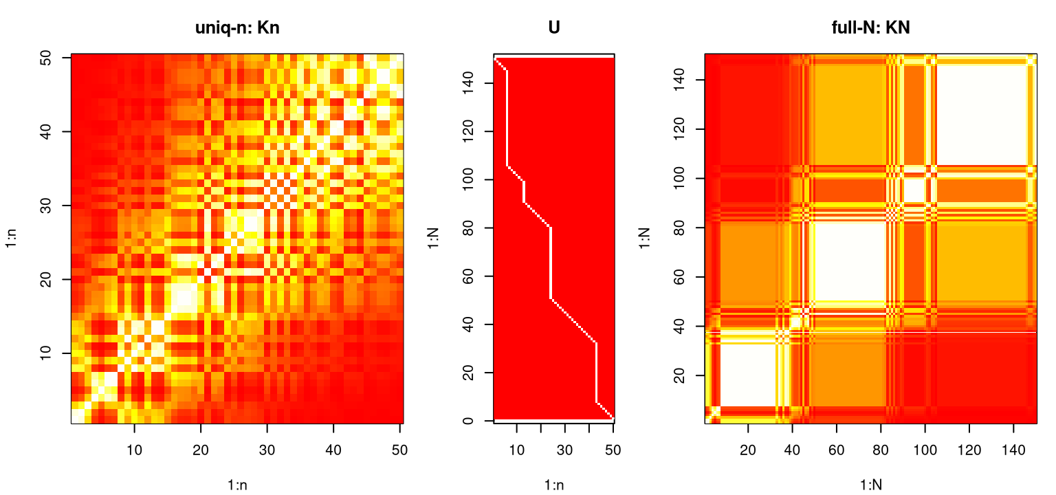
FIGURE 10.1: Example mapping \(K_n \rightarrow U \rightarrow K_N\) through Woodbury identities (10.2)–(10.3).
Storage of \(K_n\) and \(U\), which may be represented sparsely, or even implicitly, is not only more compact than \(K_N\), but the Woodbury formulas show how to calculate requisite inverse and determinants by acting on \(\mathcal{O}(n^2)\) quantities rather than \(\mathcal{O}(N^2)\) ones.
10.1.2 Efficient inference and prediction under replication
Here my aim is to make SK simultaneously more general, exact, and prescriptive, facilitating full likelihood-based inference and conditionally (on hyperparameters) exact predictive equations with the Woodbury trick. Pushing the matrix inverse identity (10.2) through to predictive equations, mapping \(\nu C_N + S_N = \nu (C_N + \Lambda_N) \equiv \nu (C_N + g \mathbb{I}_N)\) between SK and more conventional Chapter 5 notation, yields the following predictive identities:
\[\begin{align} \nu k_N^\top(x) (\nu C_N + S_N)^{-1} Y_N &= k_n^\top(x) (C_n + \Lambda_n A_n^{-1})^{-1} \bar{Y}_n \tag{10.4} \\ vk - \nu^2 k_N^\top(x) (\nu C_N + S_N)^{-1} k_N(x) &= vk - \nu k_n^\top(x) (C_n + \Lambda_n A_n^{-1})^{-1} k_n(x), \notag \end{align}\]
where \(vk \equiv \nu K_\theta(x, x)\) is used as a shorthand to save horizontal space.
In words, typical full-\(N\) predictive quantities may be calculated identically through unique-\(n\) counterparts, potentially yielding dramatic savings in computational time and space. The unique-\(n\) predictor (10.4), implicitly defining \(\mu_n(x)\) and \(\sigma_n^2(x)\) on the right-hand side(s) and updating SK (10.1), is unbiased and minimizes mean-squared prediction error (MSPE) by virtue of the fact that those properties hold for the full-\(N\) predictor on the left-hand side(s). No asymptotic or frequentist arguments are required. Crucially, no minimum data or numbers of replicates (e.g., \(a_i \geq 10\) for SK) are required to push asymptotic arguments through, although replication can still be helpful from a statistical efficiency perspective. See §10.3.1.
The same trick can be played with the concentrated log likelihood (5.8). Recall that \(K_n = C_n + A_n^{-1} \Lambda_n\), where for now \(\Lambda_n = g \mathbb{I}_n\) encoding homoskedasticity. Later I shall generalize \(\Lambda_n = \mathrm{Diag}(\lambda_1,\dots, \lambda_n)\) for the heteroskedastic setting. Using these quantities and Eqs. (10.2)–(10.3) simultaneously,
\[\begin{align} \ell &= c - \frac{N}{2} \log \hat{\nu}_N - \frac{1}{2} \sum_{i=1}^n [(a_i - 1) \log \lambda_i + \log a_i] - \frac{1}{2} \log | K_n |, \tag{10.5} \\ \mbox{where} \;\; \hat{\nu}_N &= \frac{1}{N} (Y_N^\top \Lambda_N^{-1} Y_N - \bar{Y}_n^\top A_n \Lambda_n^{-1} \bar{Y}_n + \bar{Y}_n^\top K_n^{-1} \bar{Y}_n). \notag \end{align}\]
Notice additional terms in \(\hat{\nu}_N\) compared with \(\hat{\nu}_n = n^{-1} \bar{Y}_n^\top K_n^{-1} \bar{Y}_n\). Thus \(N^{-1} Y_N^\top \Lambda_N^{-1} Y_N\) is our missing statistic for sufficiency. Since \(\Lambda_N\) is diagonal, evaluation of \(\ell\) requires just \(\mathcal{O}(n^3)\) operations beyond the \(\mathcal{O}(N)\) required for \(\bar{Y}_n\). Closed form derivative evaluations are available in \(\mathcal{O}(n^3)\) time too, facilitating library-based optimization, e.g., with BFGS.
\[\begin{align} \frac{\partial \ell}{\partial \cdot} &= \frac{N}{2} \frac{\partial ( Y_N^\top \Lambda_N^{-1} Y_N - \bar{Y}_n A_n \Lambda_n^{-1} \bar{Y}_n + n \hat{\nu}_n)}{\partial \cdot } \times (N \hat{\nu}_N)^{-1} \notag \\ &- \frac{1}{2} \sum_{i=1}^n \left[(a_i - 1) \frac{\partial \log \lambda_i}{\partial \cdot} \right] - \frac{1}{2} \mathrm{tr} \left(K_n^{-1} \frac{\partial K_n}{\partial \cdot} \right) \tag{10.6} \end{align}\]
Above, “\(\cdot\)” is a place-holder for hyperparameter(s) of interest. Fast likelihood and derivative evaluation when \(N \gg n\) can be computationally much more efficient, compared to schemes introduced in Chapter 5, yet still reside under an otherwise identical numerical umbrella.
Example: computational advantage of replication
To demonstrate the potential benefit of this Woodbury mapping, consider the following modestly-sized example based on our favorite 2d test function (§5.1.2). You may recall we leveraged replication in an extension of this example (§5.2.4) in order to control signal-to-noise behavior in repeated Rmarkdown builds. Here the response is observed at \(n=100\) unique input locations, each having a random number of replicates \(a_i \sim \mathrm{Unif}\{1,2,\dots,50\}\). Otherwise the setup is identical to previous (noisy) uses of this data-generating mechanism.
library(lhs)
Xbar <- randomLHS(100, 2)
Xbar[,1] <- (Xbar[,1] - 0.5)*6 + 1
Xbar[,2] <- (Xbar[,2] - 0.5)*6 + 1
ytrue <- Xbar[,1]*exp(-Xbar[,1]^2 - Xbar[,2]^2)
a <- sample(1:50, 100, replace=TRUE)
N <- sum(a)
X <- matrix(NA, ncol=2, nrow=N)
y <- rep(NA, N)
nf <- 0
for(i in 1:100) {
  X[(nf+1):(nf+a[i]),] <- matrix(rep(Xbar[i,], a[i]), ncol=2, byrow=TRUE)
  y[(nf+1):(nf+a[i])] <- ytrue[i] + rnorm(a[i], sd=0.01)
  nf <- nf + a[i]
}
The code below invokes mleHomGP from the hetGP package in two ways. One cripples automatic pre-processing subroutines that would otherwise calculate sufficient statistics for unique-\(n\) modeling, forcing a more cumbersome full-\(N\) calculation. Another does things the default, more thrifty unique-\(n\) way. In both cases, mleHomGP serves as a wrapper automating calls to optim with method="L-BFGS-B", furnishing implementations of log concentrated likelihood (10.5) and derivative (10.6).
Lwr <- rep(sqrt(.Machine$double.eps), 2)
Upr <- rep(10, 2)
fN <- mleHomGP(list(X0=X, Z0=y, mult=rep(1, N)), y, Lwr, Upr)
un <- mleHomGP(X, y, Lwr, Upr)
Repeating search bounds Lwr and Upr to match input dimension invokes a separable kernel, which is Gaussian by default. Execution times saved by the mleHomGP calls above show a dramatic difference.
## fN.elapsed un.elapsed
##     162.86       0.03
Calculations on unique-\(n\) quantities using Woodbury identities results in execution that’s 5429 times faster than an otherwise equivalent full-\(N\) analog. The outcome of those calculations, exemplified below through a reporting of estimated lengthscales, is nearly identical in both versions.
##     [,1]  [,2]
## fN 1.078 1.929
## un 1.078 1.929
Excepting a user-triggered SK feature offered by mlegp and DiceKriging packages on CRAN, I’m not aware of any other software package, for R or otherwise, that automatically pre-process data into a format leveraging Woodbury identities to speed up GP calculations under heavy replication. Repeated sampling is a common design tactic in the face of noisy processes, and the example above demonstrates potential for substantial computational benefit when modeling with GPs. Replication is essential when signal-to-noise features may exhibit heterogeneity across the input space. Whenever two things are changing simultaneously, a means of pinning down one – in this case variance, if only locally – can be a game-changer.
10.2 Coupled mean and variance GPs
GP kernels based on Euclidean distance (e.g., Chapter 5 or above) emit stationary processes where input–output behavior exhibits highly regular dynamics throughout the input space. Yet we saw in §9.2.2–9.3 that many data-generating mechanisms are at odds with stationarity. A process can diverge from stationary in various ways, but few are well accommodated by computationally viable modeling methodology – exceptions in Chapter 9 notwithstanding. Input-dependent variance, or heteroskedasticity, is a particular form of nonstationarity that’s increasingly encountered in stochastic simulation. A fine example is the motorcycle accident data introduced in §9.2.1. Our TGP fit to these data, shown in Figure 9.11, nicely captures noise regime changes from low, to high, to medium as inputs track from left to right. Accommodating those shifts required partitioning/hard breaks in the predictive surface which (we hoped) could be smoothed over by Markov chain Monte Carlo (MCMC) sampling from the Bayesian posterior on trees. Entertaining a smoother alternative might be worthwhile.
To lay the groundwork for a heteroskedastic GP-based alternative, and remind the reader of the setting and challenges involved, consider the following ordinary homoskedastic GP fit to these data, followed by prediction on a testing grid.
library(MASS)
hom <- mleHomGP(mcycle$times, mcycle$accel)
Xgrid <- matrix(seq(0, 60, length=301), ncol=1)
p <- predict(x=Xgrid, object=hom)
df <- data.frame(table(hom$mult))
colnames(df) <- c("reps", "howmany")
rownames(df) <- NULL
df
## reps howmany
## 1 1 66
## 2 2 22
## 3 3 3
## 4 4 2
## 5 6 1Considering the importance of separating signal from noise in this simulation experiment, perhaps it’s not surprising that the design includes moderate replication. Figure 10.2 shows the resulting predictive surface overlaid on a scatterplot of the data. The solid-black line is the predictive mean, and dashed-red lines trace out a 90% predictive interval. Output from predict.homGP separates variance in terms of epistemic/mean (p$sd2) and residual (p$nugs) estimates, which are combined in the figure to show full predictive uncertainty.
plot(mcycle)
lines(Xgrid, p$mean)
lines(Xgrid, qnorm(0.05, p$mean, sqrt(p$sd2 + p$nugs)), col=2, lty=2)
lines(Xgrid, qnorm(0.95, p$mean, sqrt(p$sd2 + p$nugs)), col=2, lty=2)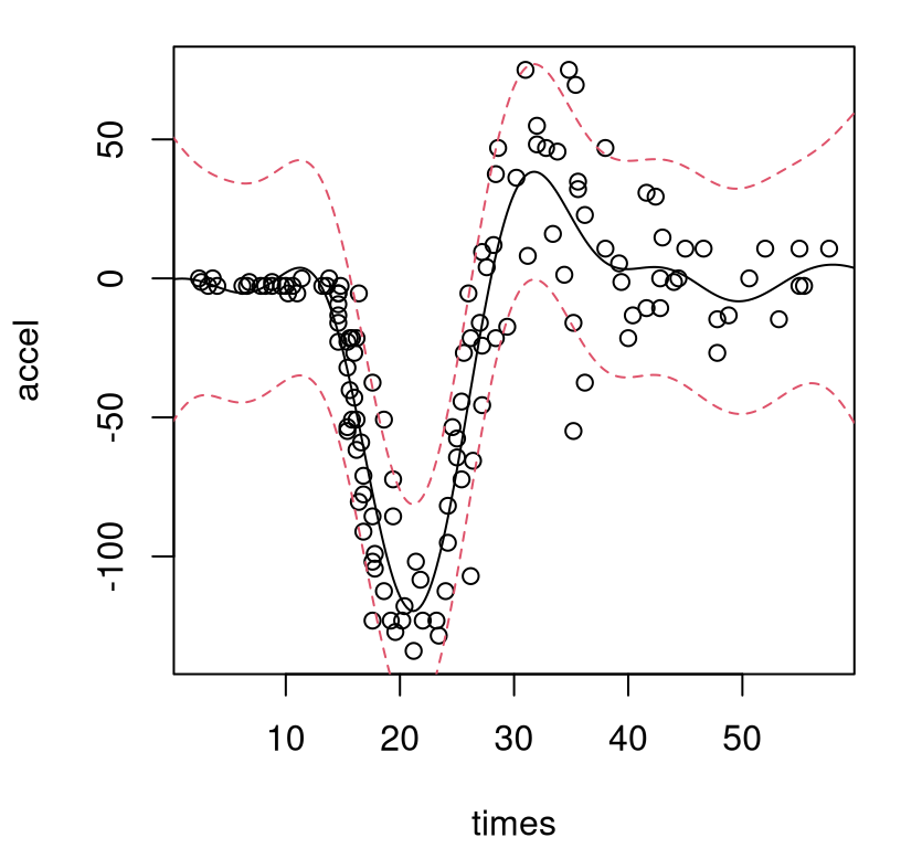
FIGURE 10.2: Homoskedastic GP fit to the motorcycle data via mean (solid-black) and 90% error-bars (dashed-red).
As in Figure 9.10, showing a (Bayesian) stationary GP, this fit is undesirable on several fronts. Not only is the variance off, but the mean is off too: it’s way too wiggly in the left-hand, pre-impact regime. Perhaps this is due to noise in the right-hand regime being incorrectly interpreted as signal, which then bleeds into the rest of the fit because the covariance structure is stationary. Learning how variance is changing is key to learning about mean dynamics. Replication is key to learning about variance.
10.2.1 Latent variance process
Heteroskedastic GP modeling targets learning the diagonal matrix \(\Lambda_N\), or its unique-\(n\) counterpart \(\Lambda_n\); see Eq. (10.4). Allowing \(\lambda_i\)-values to exhibit heterogeneity, i.e., not all \(\lambda_i = g/\nu\) as in the homoskedastic case, is easier said than done. Care is required when performing inference for such a high-dimensional parameter. SK (10.1) suggests taking \(\Lambda_n A_n^{-1} = S_n = \mathrm{Diag}(\hat{\sigma}^2_1, \dots, \hat{\sigma}^2_n)\), but that requires large numbers of replicates \(a_i\) and is anyways useless out of sample. By fitting each \(\hat{\sigma}_i^2\) separately there’s no pooling effect for interpolation/smoothing. Ankenman, Nelson, and Staum (2010) suggest the quick fix of fitting a second GP to the variance observations with “data”:
\[ (\bar{x}_1, \hat{\sigma}_1^2), (\bar{x}_2, \hat{\sigma}_2^2), \dots, (\bar{x}_n, \hat{\sigma}_n^2), \]
to obtain a smoothed variance for use out of sample.
A more satisfying approach that’s similar in spirit, coming from ML (Goldberg, Williams, and Bishop 1998) and actually predating SK by more than a decade, applies regularization that encourages a smooth evolution of variance. Goldberg et al. introduce latent (log) variance variables under a GP prior and develop an MCMC scheme performing joint inference for all unknowns, including hyperparameters for both mean and noise GPs. The overall method, which is effectively on the order of \(\mathcal{O}(TN^4)\) for \(T\) MCMC samples, is totally impractical but works well on small problems. Several authors have economized on aspects of this framework (Kersting et al. 2007; Lazaro–Gredilla and Titsias 2011) with approximations and simplifications of various sorts, but none to my knowledge have resulted in public R software.11 The key ingredient in these works, of latent variance quantities smoothed by a GP, has merits and can be effective when handled gingerly. Binois, Gramacy, and Ludkovski (2018) introduced the methodology described below.
Let \(\delta_1, \delta_2, \dots, \delta_n\) denote latent variance variables (or equivalently latent nuggets), each corresponding to one of the \(n\) unique design sites \(\bar{x}_i\) under study. It’s important to introduce latents only for the unique-\(n\) locations. A similar approach in the full-\(N\) setting, i.e., without exploiting Woodbury identities, is fraught with identifiability and numerical stability challenges. Store these latents diagonally in a matrix \(\Delta_n\) and place them under a GP prior:
\[ \Delta_n \sim \mathcal{N}_n(0, \nu_{(\delta)} (C_{(\delta)} + g_{(\delta)} A_n^{-1})). \]
Inverse exponentiated squared Euclidean distance-based correlations in \(n \times n\) matrix \(C_{(\delta)}\) are hyperparameterized by novel lengthscales \({\theta}_{(\delta)}\) and nugget \(g_{(\delta)}\). Smoothed \(\lambda_i\)-values can be calculated by plugging \(\Delta_n\) into GP mean predictive equations:
\[\begin{equation} \Lambda_n = C_{(\delta)} K_{(\delta)}^{-1} \Delta_n, \quad \mbox{ where } \quad K_{(\delta)} = (C_{(\delta)} + g_{(\delta)} A_n^{-1}). \tag{10.7} \end{equation}\]
Smoothly varying \(\Lambda_n\) generalize both \(\Lambda_n = g \mathbb{I}_n\) from a homoskedastic setup, and moment-estimated \(S_n\) from SK. Hyperparameter \(g_{(\delta)}\) is a nugget of nuggets, controlling the smoothness of \(\lambda_i\)’s relative to \(\delta_i\)’s; when \(g_{(\delta)} = 0\) the \(\lambda_i\)’s interpolate \(\delta_i\)’s. Although the formulation above uses a zero-mean GP, a positive nonzero mean \(\mu_{(\delta)}\) may be preferable for variances. The hetGP package automates a classical plugin estimator \(\hat{\mu}_{(\delta)} = \Delta_n^\top K_{(\delta)}^{-1} \Delta_n (1_n^\top K_{(\delta)}^{-1} 1_n)^{-1}\). See exercise #2 from §5.5 and take intercept-only \(\beta\). This seemingly simple twist unnecessarily complicates the remainder of the exposition, so I shall continue to assume zero mean throughout.
Variances must be positive, and the equations above give nonzero probability to negative \(\delta_i\) and \(\lambda_i\)-values. One solution is to threshold latent variances at zero. Another is to model \(\log \Delta_n\) in this way instead. The latter option, guaranteeing positive variance after exponentiating, is the default in hetGP but both variations are implemented. Differences in empirical performance and mathematical development are slight. Modeling \(\log \Delta_n\) makes derivative expressions a little more complicated after applying the chain rule, so our exposition here shall continue with the simpler un-logged variation. Logged analogs are left to an exercise in §10.4.
So far the configuration isn’t much different than what Goldberg, Williams, and Bishop (1998) described more than twenty years ago, except for an emphasis here on unique-\(n\) latents. Rather than cumbersome MCMC, Binois et al. describe how to stay within a (Woodbury) MLE framework, by defining a joint log likelihood over both mean and variance GPs:
\[\begin{align} \tilde{\ell} &= c - \frac{N}{2} \log \hat{\nu}_N - \frac{1}{2} \sum\limits_{i=1}^n \left[(a_i - 1)\log \lambda_i + \log a_i \right] - \frac{1}{2} \log |K_n| \tag{10.8} \\ &\quad - \frac{n}{2} \log \hat{\nu}_{(\delta)} - \frac{1}{2} \log |K_{(\delta)}|. \notag \end{align}\]
Maximization is assisted by closed-form derivatives which may be evaluated with respect to all unknown quantities in \(\mathcal{O}(n^3)\) time. For example, the derivative with respect to latent \(\Delta_n\) may be derived as follows.
\[ \begin{aligned} \frac{\partial \tilde{\ell}}{\partial \Delta_n} &= \frac{\partial \Lambda_n}{\partial \Delta_n} \frac{\partial \tilde{\ell}}{\partial \Lambda_n} = C_{(\delta)} K_{(\delta)}^{-1} \frac{\partial \tilde{\ell}}{\partial \Lambda_n} - \frac{K_{(\delta)}^{-1} \Delta_n}{\hat{\nu}_{(\delta)}} \\ \mbox{ where } \quad \frac{\partial \tilde{\ell}}{\partial \lambda_i} &= \frac{N}{2} \times \frac{\frac{ a_i \hat{\sigma}_i^2} {\lambda_i^2} + \frac{(K_n^{-1} \bar{Y}_n)^2_i}{a_i}}{\hat{\nu}_N} - \frac{a_i - 1}{2\lambda_i} - \frac{1}{2a_i} (K_n)_{i, i}^{-1} \end{aligned} \]
Recall that \(\hat{\sigma}_i^2 = \frac{1}{a_i} \sum_{j=1}^{a_i} (y_i^{(j)} - \bar{y}_j)^2\). So an interpretation of Eq. (10.8) is as an extension of SK estimates \(\hat{\sigma}_i^2\) at \(\bar{x}_i\). In contrast with SK, GP smoothing provides regularization needed in order to accommodate small numbers of replicates, even \(a_i = 1\) in spite of \(\hat{\sigma}_i^2 = 0\). In this single replicate case, \(y_i\) still contributes to local variance estimates through the rest of Eq. (10.8). Note that Eq. (10.8) is not constant in \(\delta_i\); in fact it depends (10.7) on all of \(\Delta_n\). Smoothing may be entertained on other quantities, e.g., \(\Lambda_n \hat{\nu}_N = C_{(\delta)} K_{(\delta)}^{-1} S_n^2\) presuming \(a_i > 1\), resulting in smoothed moment-based variance estimates in the style of SK (Kamiński 2015; W. Wang and Chen 2016). There may similarly be scope for bypassing a latent GP noise process with a SiNK predictor (M. Lee and Owen 2015) by taking
\[ \Lambda_n = \rho(\bar{X}_n)^{-1} C_{(\delta)} K_{(\delta)}^{-1}\Delta_n \quad \mbox{ with } \quad \rho(x) = \sqrt{\hat{\nu}_{(\delta)} c_{(\delta)}(x)^\top K_{(\delta)}^{-1} c_{(\delta)}(x)}, \]
or alternatively through \(\log \Lambda_n\).
Binois, Gramacy, and Ludkovski (2018) show that \(\tilde{\ell}\) in Eq. (10.8) is maximized when \(\Delta_n = \Lambda_n\) and \(g_{(\delta)}=0\). In other words, smoothing latent nuggets (10.7) is unnecessary at the MLE. However, intermediate smoothing is useful as a device in three ways: 1) connecting SK to Goldberg’s latent representation; 2) annealing to avoid local minima; and 3) yielding a smooth solution when the numerical optimizer is stopped prematurely, which may be essential in big data (large unique-\(n\)) contexts.
It’s amazing that a simple optim call can be brought to bear in such a high dimensional setting. Thoughtful initialization helps. Residuals from an initial homoskedastic fit can prime \(\Delta_n\)-values. For more implementation details and options, see Section 3.3 of Binois and Gramacy (2018). \(\mathcal{O}(n)\) latent variables can get big, especially as higher dimensional examples demand training datasets with more unique inputs. This is where replication really shines, inducing a likelihood that locks in high-replicate latents early on in the optimization. The Woodbury trick (§10.1.1) is essential here. Beyond simply being inefficient, having multiple latent \(\delta_i^{(j)}\) at unique \(\bar{x}_i\) corrupts optimization by inserting numerical weaknesses into the log likelihood.
Goldberg, Williams, and Bishop (1998)’s MCMC is more forgiving in this regard. MC is a robust, if (very) slowly converging, numerical procedure. Besides that nuance favoring a Woodbury unique-\(n\) formulation, the likelihood surface is exceedingly well behaved. Critics have suggested expectation maximization (EM) to integrate out latent variances. But this simply doesn’t work except on small problems; EM represents nearly as much work as MCMC. Kersting et al. (2007) and Quadrianto et al. (2009) keyed into this fact a decade ago, but without the connection to SK, replication, and the Woodbury trick.
10.2.2 Illustrations with hetGP
Passages below take the reader through a cascade of examples illustrating hetGP: starting simply by returning to the motorcycle accident data, and progressing up though real-simulation examples from epidemiology to Bayesian model selection and inventory management.
Motorcycle accident data
The code below shows how to fit a heteroskedastic, coupled mean and variance GP, with smoothed initialization and Matérn covariance structure. This is but one of several potential ways to obtain a good fit to these data using the methods provided by hetGP.
het <- mleHetGP(mcycle$times, mcycle$accel, covtype="Matern5_2",
  settings=list(initStrategy="smoothed"))
het$time
## elapsed
## 0.684Time required to perform the requisite calculations is trivial, although admittedly this isn’t a big problem. Built-in predict.hetGP works the same as its .homGP cousin, illustrated earlier.
p2 <- predict(het, Xgrid)
ql <- qnorm(0.05, p2$mean, sqrt(p2$sd2 + p2$nugs))
qu <- qnorm(0.95, p2$mean, sqrt(p2$sd2 + p2$nugs))
Figure 10.3, shows the resulting predictive surface in two views. The first view, in the left panel, complements Figure 10.2. Observe how the surface is heteroskedastic, learning the low-variance region in the first third of inputs and higher variance for the latter two-thirds. As a consequence of being able to better track signal-to-noise over the input space, extraction of signal (particularly for the first third of times) is better than in the homoskedastic case.
par(mfrow=c(1,2))
plot(mcycle, ylim=c(-160, 90), ylab="acc", xlab="time",
  main="predictive surface")
lines(Xgrid, p2$mean)
lines(Xgrid, ql, col=2, lty=2)
lines(Xgrid, qu, col=2, lty=2)
plot(Xgrid, p2$nugs, type="l", ylab="s2", xlab="times",
  main="variance surface", ylim=c(0, 2e3))
points(het$X0, sapply(find_reps(mcycle[,1], mcycle[,2])$Zlist, var),
  col=3, pch=20)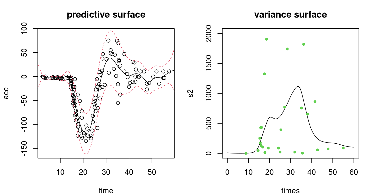
FIGURE 10.3: Heteroskedastic GP fit to the motorcycle data. Left panel shows the predictive distribution via mean (solid-black) and 90% error-bars (dashed-red); compare to Figure 10.2. Right panel shows the estimated variance surface and moment-based estimates of variance (green dots).
The second view, in the right panel of the figure, provides more detail on latent variances. Predictive uncertainty is highest for the middle third of times, which makes sense because this is where the whiplash effect is most prominent. Green dots in that panel indicate moment-based estimates of variance obtained from a limited number of replicates \(a_i > 1\) available for some inputs. (There are nowhere near enough for an SK-like approach.) Observe how the black curve, smoothing latent variance values \(\Delta_n\), extracts the essence of the pattern of those values. This variance fit uses the full dataset, leveraging smoothness of the GP prior to incorporate responses at inputs with only one replicate, which in this case represents most of the data.
Susceptible, infected, recovered
Hu and Ludkovski (2017) describe a 2d simulation arising from the spread of an epidemic in a susceptible, infected, recovered (SIR) setting, a common stochastic compartmental model. Inputs are \((S_0, I_0\)), the numbers of initial susceptible and infected individuals. Output is the total number of newly infected individuals which may be calculated by approximating
\[ f(x) := \mathbb{E}\left\{ S_0 - \lim_{T \to \infty} S_T \mid (S_0,I_0,R_0) = x \right\} = \gamma \mathbb{E} \left\{ \int_0^\infty I_t \,dt \mid x \right\} \]
under continuous time Markov dynamics with transitions \(S + I \rightarrow 2I\) and \(I \rightarrow R\). The resulting surface is heteroskedastic and has some high noise regions. Parts of the input space represent volatile regimes wherein random chance intimately affects whether or not epidemics spread quickly or die out.
A function generating the data for standardized inputs in the unit square (corresponding to coded \(S_0\) and \(I_0\)) is provided by sirEval in the hetGP package. Output is also standardized. Consider a space-filling design of \(n=200\) unique runs under random replication \(a_i \sim \mathrm{Unif}\{1,\dots, 100\}\). Coordinate \(x_1\) represents the initial number of infecteds \(I_0\), and \(x_2\) the initial number of susceptibles \(S_0\).
Xbar <- randomLHS(200, 2)
a <- sample(1:100, nrow(Xbar), replace=TRUE)
X <- matrix(NA, ncol=2, nrow=sum(a))
nf <- 0
for(i in 1:nrow(Xbar)) {
  X[(nf+1):(nf+a[i]),] <- matrix(rep(Xbar[i,], a[i]), ncol=2, byrow=TRUE)
  nf <- nf + a[i]
}
nf
## [1] 10407The result is a full dataset with about ten thousand runs. Code below gathers responses – expected total number of infecteds at the end of the simulation – at each input location in the design, including replicates.
Code below fits our hetGP model. By default, lengthscales for the variance GP (\(\theta_{(\delta)}\)) are linked to those from the mean GP (\(\theta\)), requiring that the former be a scalar multiple \(k>1\) of the latter. That feature can be switched off, however, as illustrated below. Specifying scalar lower and upper signals an isotropic kernel.
## elapsed
##   195.5
Around 200 seconds are needed to train the model. To visualize the resulting predictive surface, code below creates a dense grid in 2d and calls predict.hetGP on the fit object.
xx <- seq(0, 1, length=100)
XX <- as.matrix(expand.grid(xx, xx))
psir <- predict(fit, XX)
vsir <- psir$sd2 + psir$nugs
The left panel of Figure 10.4 captures predictive means; the right panel shows predictive standard deviation. Text overlaid on the panels indicates the location of the training data inputs and the number of replicates observed thereupon.
par(mfrow=c(1,2))
image(xx, xx, matrix(psir$mean, ncol=100), xlab="S0", ylab="I0",
  col=cols, main="mean infected")
text(Xbar, labels=a, cex=0.5)
image(xx, xx, matrix(sqrt(vsir), ncol=100), xlab="S0", ylab="I0",
  col=cols, main="sd infected")
text(Xbar, labels=a, cex=0.5)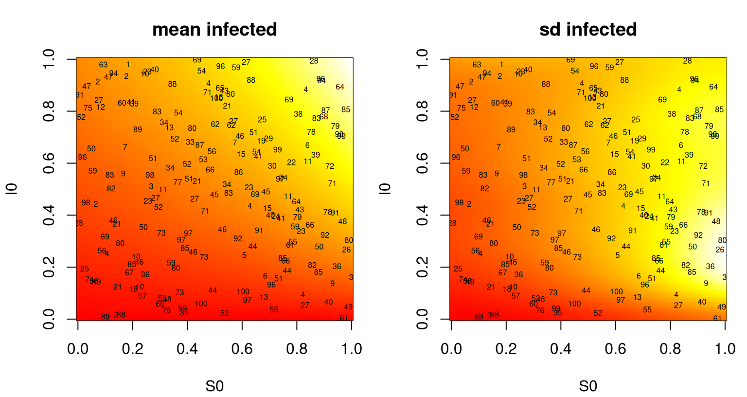
FIGURE 10.4: Heteroskedastic GP fit to the SIR data showing predictive mean surface (left) and estimated standard deviation (right). Text in both panels shows numbers of replicates in training.
Notice in the figure how means are changing more slowly than variances. Un-linking their lengthscales was probably the right move. Interpreting the mean surface, the number of infecteds is maximized when initial \(S_0\) and/or \(I_0\) is high. That makes sense. Predictive uncertainty in total number of infecteds is greatest when there’s a large number of initial susceptible individuals, but a moderate number of initial infecteds. That too makes sense. A moderate injection of disease into a large, vulnerable population could swell to spell disaster.
Bayesian model selection
Model selection by Bayes factor (BF) is known to be sensitive to hyperparameter choice in hierarchical models, which is further complicated and obscured by MC evaluation injecting a substantial source of noise. To study BF surfaces in such settings, Franck and Gramacy (2020) propose treating expensive BF evaluations, with MCMC say, as a (stochastic) computer simulation experiment. BF calculations at a space-filling design in the input/hyperparameter space can be used to map and thus better understand sensitivity of model selection to those settings.
As a simple warm-up example, consider an experiment described in Sections 3.3–3.4 of Gramacy and Pantaleo (2010) where BF calculations determine whether data is leptokurtic (Student-\(t\) errors) or not (simply Gaussian). Here we study BF approximation as a function of prior parameterization on the Student-\(t\) degrees of freedom parameter \(\nu\), which Gramacy and Pantaleo took as \(\nu \sim \mathrm{Exp}(\theta = 0.1)\). Their intention was to be diffuse, but ultimately they lacked an appropriate framework for studying sensitivity to this choice. Franck and Gramacy (2020) designed a grid of \(\theta\)-values, evenly spaced in \(\log_{10}\) space from \(10^{-3}\) to \(10\) spanning “solidly Student-\(t\)” (even Cauchy) to “essentially Gaussian” prior specifications for \(\mathbb{E}\{\nu\}\). Each \(\theta_i\) gets its own reversible jump MCMC simulation (Richardson and Green 1997), as automated by blasso in the monomvn package (Gramacy 2018b) on CRAN, taking about 36 minutes on a 3.20GHz Intel Core i7 processor. Converting those posterior draws into \(\mathrm{BF}_{\mathrm{St}\mathcal{N}}^{(i)}\) evaluations follows a post-processing scheme described by Jacquier, Polson, and Rossi (2004). To better understand MC variability in those calculations, ten replicates of BFs under each hyperparameter setting \(\theta_i\) were simulated. Collecting 200 BFs in this way takes about 120 hours. These data are saved in the hetGP package for later analysis.
BF evaluation by MCMC is notoriously unstable. We shall see that even in log-log space, the \(\mathrm{BF}_{\mathrm{St}\mathcal{N}}\) process is not only heteroskedastic but also has heavy tails. Consequently Franck and Gramacy (2020) fit a heteroskedastic Student-\(t\) process (TP). Details are provided in Section 3.2 of Binois and Gramacy (2018) and Chung et al. (2019) who describe several other extensions including an additional layer of latent variables to handle missing data, and a scheme to enforce a monotonicity property. Both are motivated by a challenging class of inverse problems involved in characterizing spread of influenza.
bfs1 <- mleHetTP(X=list(X0=log10(thetas), Z0=colMeans(log(bfs)),
  mult=rep(nrow(bfs), ncol(bfs))), Z=log(as.numeric(bfs)), lower=1e-4,
  upper=5, covtype="Matern5_2")
Predictive evaluations may be extracted on a grid in the input space …
… and visualized in Figure 10.5. Each open circle is a \(\mathrm{BF}_{\mathrm{St}\mathcal{N}}\) evaluation, plotted in \(\log_{10}\)–\(\log_e\) space.
matplot(log10(thetas), t(log(bfs)), col=1, pch=21, ylab="log(bf)")
lines(log10(dx), p$mean)
lines(log10(dx), p$mean + 2*sqrt(p$sd2 + p$nugs), col=2, lty=2)
lines(log10(dx), p$mean - 2*sqrt(p$sd2 + p$nugs), col=2, lty=2)
legend("topleft", c("hetTP mean", "hetTP interval"), col=1:2, lty=1:2)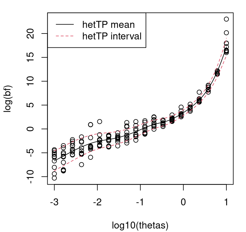
FIGURE 10.5: Heteroskedastic TP fit to Bayes factor data under exponential hyperprior.
It bears repeating that the \(\mathrm{BF}_{\mathrm{St}\mathcal{N}}\) surface is heteroskedastic, even after log transform, and has heavy tails. A take-home message from these plots is that BF surfaces can be extremely sensitive to hierarchical modeling hyperparameterization. When \(\theta\) is small, the Student-\(t\) (\(\mathrm{BF}_{\mathrm{St}\mathcal{N}} < 1\)) is essentially a foregone conclusion, whereas if \(\theta\) is large the Gaussian (\(\mathrm{BF}_{\mathrm{St}\mathcal{N}} > 1\)) is. This is a discouraging result for model selection with BFs in this setting: a seemingly innocuous hyperparameter is essentially determining the outcome of selection.
Although the computational burden involved in this experiment – 120 hours – is tolerable, extending the idea to higher dimensions is problematic. Suppose one wished to entertain \(\nu \sim \mathrm{Gamma}(\alpha, \beta)\), where the \(\alpha=1\) case reduces to \(\nu \sim \mathrm{Exp}(\beta \equiv \theta)\) above. Over a similarly dense hyperparameter grid, runtime would balloon to more than one hundred days which is clearly unreasonable. Instead it makes sense to build a surrogate model from a more limited space-filling design and use the resulting posterior predictive surface to understand variability in BFs in the hyperparameter space. Five replicate responses on a size \(n=80\) LHS in \(\alpha \times \beta\)-space were obtained for a total of \(N=400\) MCMC runs. These data are provided as bfs.gamma in the bfs data object in hetGP.
A similar hetTP fit may be obtained with …
bfs2 <- mleHetTP(X=list(X0=log10(D), Z0=colMeans(log(bfs)),
  mult=rep(nrow(bfs), ncol(bfs))), Z=log(as.numeric(bfs)),
  lower=rep(1e-4, 2), upper=rep(5, 2), covtype="Matern5_2")
… followed by predictions on a dense grid in the 2d input space.
dx <- seq(0, 1, length=100)
dx <- 10^(dx*4 - 3)
DD <- as.matrix(expand.grid(dx, dx))
p <- predict(bfs2, log10(DD))
Figure 10.6 shows the outcome of that experiment: mean surface in the left panel and standard deviation in the right. Numbers overlaid indicate average \(\mathrm{BF}_{\mathrm{St}\mathcal{N}}\) obtained for the five replicates at each input location. Contours in the left panel correspond to levels in the so-called Jeffreys scale.
par(mfrow=c(1,2))
mbfs <- colMeans(bfs)
image(log10(dx), log10(dx), t(matrix(p$mean, ncol=length(dx))), col=cols,
  xlab="log10 alpha", ylab="log10 beta",  main="mean log BF")
text(log10(D[,2]), log10(D[,1]), signif(log(mbfs), 2), cex=0.5)
contour(log10(dx), log10(dx), t(matrix(p$mean, ncol=length(dx))),
  levels=c(-5,-3,-1,0,1,3,5), add=TRUE, col=4)
image(log10(dx), log10(dx), t(matrix(sqrt(p$sd2 + p$nugs),
  ncol=length(dx))), co =cols, xlab="log10 alpha",
  ylab="log10 beta", main="sd log BF")
text(log10(D[,2]), log10(D[,1]), signif(apply(log(bfs),2,sd), 2), cex=0.5)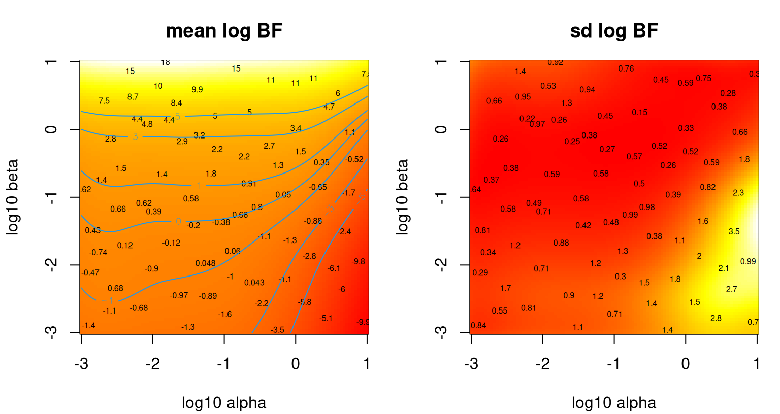
FIGURE 10.6: Heteroskedastic TP fit to the Bayes factor data under Gamma hyperprior.
The story here is much the same as before in terms of \(\beta\), which maps to \(\theta\) in the earlier experiment, especially near \(\alpha=1\), or \(\log_{10} \alpha=0\) where equivalence is exact. The left panel shows that along that slice one can get just about any model selection conclusion one wants. Smaller \(\alpha\)-values tell a somewhat more nuanced story, however. A rather large range of smaller \(\alpha\)-values leads to somewhat less sensitivity in the outcome, except when \(\beta\) is quite large. Apparently, having a small \(\alpha\) setting is essential if data are going to have any influence on model selection with BFs. The right panel shows that variances are indeed changing over the input space, justifying the heteroskedastic surrogate.
Inventory management
The assemble-to-order (ATO) problem (Hong and Nelson 2006) involves a queuing simulation targeting inventory management scenarios. At its heart it’s an optimization or reinforcement learning problem, however here I simply treat it as a response surface to be learned. Although the signal-to-noise ratio is relatively high, ATO simulations are known to be heteroskedastic, e.g., as illustrated by documentation for the MATLAB® library utilized for simulations (J. Xie, Frazier, and Chick 2012).
The setting is as follows. A company manufactures \(m\) products. Products are built from base parts called items, some of which are “key” in that the product can’t be built without them. If a random request comes in for a product that’s missing a key item, a replenishment order is executed and filled after random delay. Holding items in inventory is expensive, so balance must be struck between inventory costs and revenue. Binois, Gramacy, and Ludkovski (2018) describe an experiment under target stock vector inputs \(b \in \{0,1,\dots,20\}^8\) for eight items.
Code below replicates results from that experiment, which entail a uniform design of size \(n_{\mathrm{tot}}=2000\) in 8d with ten replicates for a total design size of \(N_{\mathrm{tot}}=20000\). A training–testing partition was constructed by randomly selecting \(n=1000\) unique locations and replicates \(a_i \sim \mathrm{Unif}\{1,\dots,10\}\) thereupon. The ato data object in hetGP contains one such random partition, which is subsequently coded into the unit cube \([0,1]^8\). Further detail is provided in package documentation for the ato data object.
Actually that object provides two testing sets. One is a genuine out-of-sample set, where testing sites are exclusive of training locations. The other is replicate based, involving those \(10-a_i\) runs not selected for training. The training set is large, making MLE calculations slow, so the ato object additionally provides a fitted model for comparison. Examples in the ato documentation file provide code which may be used to reproduce that fit or to create a new one based on novel training–testing partitions.
##            n            N time.elapsed
##         1000         5594         8584
Storing these objects facilitates fast illustration of prediction and out-of-sample comparison. It also provides a benchmark against which a more thoughtful sequential design scheme, introduced momentarily in §10.3.1, can be judged. Code below performs predictions at the held-out testing sites and then calculates a pointwise proper score (Eq. (27) from Gneiting and Raftery 2007) with ten replicates observed at each of those locations. Higher scores are better.
phet <- predict(out, Xtest)
phets2 <- phet$sd2 + phet$nugs
mhet <- as.numeric(t(matrix(rep(phet$mean, 10), ncol=10)))
s2het <- as.numeric(t(matrix(rep(phets2, 10), ncol=10)))
sehet <- (unlist(t(Ztest)) - mhet)^2
sc <- - sehet/s2het - log(s2het)
mean(sc)
## [1] 3.396A similar calculation may be made for held-out training replicates, shown below. These are technically out-of-sample, but accuracy is higher since training data were provided at these sites.
phet.out <- predict(out, Xtrain.out)
phets2.out <- phet.out$sd2 + phet.out$nugs
s2het.out <- mhet.out <- Ztrain.out
for(i in 1:length(mhet.out)) {
  mhet.out[[i]] <- rep(phet.out$mean[i], length(mhet.out[[i]]))
  s2het.out[[i]] <- rep(phets2.out[i], length(s2het.out[[i]]))
}
mhet.out <- unlist(t(mhet.out))
s2het.out <- unlist(t(s2het.out))
sehet.out <- (unlist(t(Ztrain.out)) - mhet.out)^2
sc.out <- - sehet.out/s2het.out - log(s2het.out)
mean(sc.out)
## [1] 5.086Those two testing sets may be combined to provide a single score calculated on the entire corpus of held-out data. The result is a compromise between the two score statistics calculated earlier.
## [1] 3.926Binois, Gramacy, and Ludkovski (2018) repeated that training–testing partition one hundred times to provide score boxplots which may be compared to simpler (e.g., homoskedastic) GP-based approaches. I shall refer the curious reader to Figure 2 in that paper for more details. To make a long story short, fits accommodating heteroskedasticity in the proper way – via coupled GPs and fully likelihood-based inference – are superior to all other (computationally tractable) ways entertained.
10.3 Sequential design
A theme from Chapter 6 is that design for GPs has a chicken-or-egg problem. Model-based designs are hyperparameter dependent, and data are required to estimate parameters. Space-filling designs may be sensible but are often sub-optimal. It makes sense to proceed sequentially (§6.2). That was for the ordinary, homoskedastic/stationary GPs of Chapter 5. Now noise is high and possibly varying regionally. Latent variables must be optimized. Replication helps, but how much and where?
The following characterizes the state of affairs as regards replication in experiment design for GP surrogates. In low/no-noise settings and under the assumption of stationarity (i.e., constant stochasticity), replication is of little value. Yet no technical result precludes replication except in deterministic settings. Conditions under which replicating is an optimal design choice are, until recently, unknown. When replicating, as motivated perhaps by an abundance of caution, one spot is sufficient because under stationarity the variance is the same everywhere.
Even less is known about heteroskedastic settings. Perhaps more replicates may be needed in high-variance regions? Ankenman, Nelson, and Staum (2010) show that once you have a design, under a degree of replication “large enough” to trust its moment-based estimates of spatial variance, new replicates can be allocated optimally. But what use are they if you already have “enough”, and what about the quagmire when you learn that you need fewer than you already have? (More on that in §10.3.2.) On the other hand, if means are changing quickly – but otherwise exhibit stationary dynamics – might it help to concentrate design acquisitions where noise is lower so that signal-learning is relatively cheap in replication terms? One thing’s for sure: we’d better proceed sequentially. Before data are collected, regions of high or low variance are unknown.
Details driving such trade-offs, requisite calculations and what can be learned from them, depend upon design criteria. Choosing an appropriate criterion depends upon the goal of modeling and/or prediction. §10.3.1–10.3.3 concentrate on predictive accuracy under heteroskedastic models, extending §6.2.2. §10.3.4 concludes with pointers to recent work in Bayesian optimization (extending §7.2), level set finding, and inverse problems/calibration (§8.1).
10.3.1 Integrated mean-squared prediction error
Integrated mean-squared prediction error (IMSPE) is a common model-based design criterion, whether for batch design (§6.1.2) or in sequential application as embodied by ALC (§6.2.2). Here our focus is sequential, however many calculations, and their implementation in hetGP, naturally extend to the batch setting as already illustrated in §6.1.2. IMSPE is predictive variance averaged over the input space, which must be minimized.
\[\begin{equation} I_{n+1}(x_{n+1}) \equiv \mathrm{IMSPE}(\bar{x}_1, \dots, \bar{x}_n, x_{n+1}) = \int_{x \in \mathcal{X}} \breve{\sigma}^2_{n+1}(x) \, dx \tag{10.9} \end{equation}\]
Recall that \(\breve{\sigma}^2(x)\) is nugget-free predictive variance (7.5), capturing only epistemic uncertainty about the latent random field (§5.3.2). IMSPE above is expressed in terms of unique-\(n\) inputs for reasons that shall be clarified shortly. Following the right-hand side of Eq. (10.4), we have
\[\begin{equation} \breve{\sigma}_{n+1}^2(x) = \nu(1 - k_{n+1}^\top(x) (C_{n+1} + \Lambda_{n+1} A_{n+1}^{-1})^{-1} k_{n+1}(x)). \tag{10.10} \end{equation}\]
Re-expression for full-\(N\) is straightforward. The next design location, \(x_{N+1}\), may be a new unique location \((\bar{x}_{n+1})\) or a repeat of an existing one (i.e., one of \(\bar{x}_1, \dots, \bar{x}_n\)).
Generally speaking, integral (10.9) requires numerical evaluation (Seo et al. 2000; Gramacy and Lee 2009; Gauthier and Pronzato 2014; Gorodetsky and Marzouk 2016; MT Pratola et al. 2017). §6.2.2 offers several examples; or Ds2x=TRUE in the tgp package (Gramacy and Taddy 2016) – see §9.2.2. Both offer approximations based on sums over a reference set, with the latter providing additional averaging over MCMC samples from the posterior of hyperparameters and trees. Conditional on GP hyperparameters, and when the study region \(\mathcal{X}\) is an easily integrable domain such as a hyperrectangle, requisite integration may be calculated in closed form. Although examples exist elsewhere in the literature (e.g., Ankenman, Nelson, and Staum 2010; Anagnostopoulos and Gramacy 2013; Burnaev and Panov 2015; Leatherman, Santner, and Dean 2017) for particular cases, hetGP provides the only implementation on CRAN that I’m aware of. Binois et al. (2019) extend many of those calculations to the Woodbury trick, showing for the first time how choosing a replicate can be optimal in active learning/sequential design.
The closed form solution leverages that IMSPE is similar to an expectation over covariance functions.
\[\begin{align} I_{n+1}(x_{n+1}) &= \mathbb{E} \{ \breve{\sigma}^2_{n+1}(X) \} = \mathbb{E} \{K_\theta(X, X) - k_{n+1}^\top(X) K_{n+1}^{-1} k_{n+1}(X) \} \tag{10.11} \\ &= \mathbb{E} \{K_\theta(X,X)\} - \mathrm{tr}(K_{n+1}^{-1} W_{n+1}), \notag \end{align}\]
where \(W_{ij} = \int_{x \in \mathcal{X}} k(x_i, x) k(x_j, x)\, dx\). Closed forms for \(W_{ij}\) exist with \(\mathcal{X}\) being a hyperrectangle. Notice that \(K_{n+1}\) depends on the number of replicates per unique design element, so this representation includes a tacit dependence on noise level and replication counts \(a_1, \ldots, a_n\). Binois et al. (2019) provide forms for several popular covariance functions, including the Matérn. In the case of the separable Gaussian:
\[ W_{ij}= \prod_{k=1}^m \dfrac{\sqrt{2\pi \theta_k} }{4} \exp\left\{-\dfrac{(x_{ik}-x_{jk})^2}{2 \theta_k}\right\} \left[\mathrm{erf}\left\{\dfrac{2-(x_{ik}+x_{jk})}{\sqrt{2 \theta_k}}\right\}+ \mathrm{erf}\left\{\dfrac{x_{ik}+x_{jk}}{\sqrt{ 2\theta_k}}\right\} \right]. \]
Above, \(\mathrm{erf}\) is the error function which is similar to the standard Gaussian CDF. Gradients are also available in closed form, which is convenient for fast library-based optimization as a means of solving for acquisitions. Partitioned inverse equations (6.8) make evaluation of \(I_{n+1}(x_{n+1})\) and its derivative quadratic in \(n\). See Binois et al. for details.
To investigate how replication can be favored by IMSPE, consider the following scenario(s). Let \(r(x)\) denote a belief about extrinsic variance. Choice of \(r(x)\) is arbitrary. In practice we shall use estimated \(r(x) = \breve{\sigma}_n(x)\), as above. However this illustration contrives two simpler \(r(x)\), primarily for pedagogical purposes, based on splines that agree at five knots. Knot locations could represent design sites \(\bar{x}_i\) where potentially many replicate responses have been observed.
rn <- c(6, 4, 5, 6.5, 5)
X0 <- matrix(seq(0.2, 0.8, length.out=length(rn)))
X1 <- matrix(c(X0, 0.3, 0.4, 0.9, 1))
Y1 <- c(rn, 4.7, 4.6, 6.3, 4.5)
r1 <- splinefun(x=X1, y=Y1, method="natural")
X2 <- matrix(c(X0, 0.0, 0.3))
Y2 <- c(rn, 7, 2)
r2 <- splinefun(x=X2, y=Y2, method="natural")
Figure 10.7 provides a visual of these two hypotheses evaluated on a testing grid. Below I shall refer to these surfaces as “green” and “blue”, respectively, referencing the colors from the figure. Knots are shown as red open circles.
xx <- matrix(seq(0, 1, by=0.005))
plot(X0, rn, xlab="x", ylab="r(x)", xlim=c(0,1), ylim=c(2,8), col=2)
lines(xx, r1(xx), col=3)
lines(xx, r2(xx), col=4)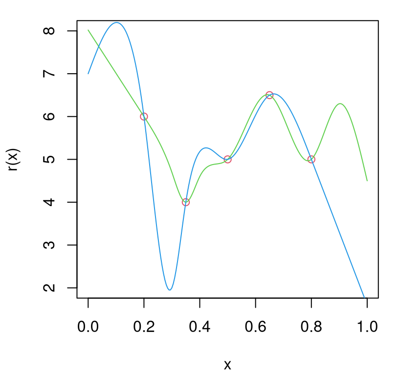
FIGURE 10.7: Two example \(r(x)\) variance surfaces based on splines with knots as open red circles.
The code below implements Eq. (10.11) for generic variance function r, like one of our splines from above. It uses internal hetGP functions such as Wij and cov_gen. (We shall illustrate the intended hooks momentarily; these low-level functions are of value here in this toy example.)
IMSPE.r <- function(x, X0, theta, r) {
  x <- matrix(x, nrow = 1)
  Wijs <- Wij(mu1=rbind(X0, x), theta=theta, type="Gaussian")
  K <- cov_gen(X1=rbind(X0, x), theta=theta)
  K <- K + diag(apply(rbind(X0, x), 1, r))
  return(1 - sum(solve(K)*Wijs))
}
Next, apply this function on a grid for each \(r(x)\), green and blue …
imspe1 <- apply(xx, 1, IMSPE.r, X0=X0, theta=0.25, r=r1)
imspe2 <- apply(xx, 1, IMSPE.r, X0=X0, theta=0.25, r=r2)
xstar1 <- which.min(imspe1)
xstar2 <- which.min(imspe2)
… and visualize in Figure 10.8. The \(x\)-locations of the knots – our hypothetical unique design sites \(\bar{x}_1,\dots, \bar{x}_n\) – are indicated as dashed red vertical bars.
plot(xx, imspe1, type="l", col=3, ylab="IMSPE", xlab="x", ylim=c(0.6, 0.7))
lines(xx, imspe2, col=4)
abline(v=X0, lty=3, col='red')
points(xx[xstar1], imspe1[xstar1], pch=23, bg=3)
points(xx[xstar2], imspe2[xstar2], pch=23, bg=4)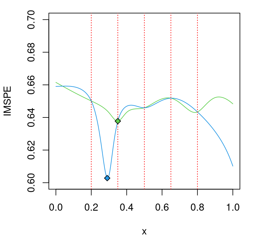
FIGURE 10.8: IMSPE surfaces from the two \(r(x)\) in Figure 10.7; knots indicated as red vertical dashed lines.
In the figure, the blue variance hypothesis is minimized at a novel \(\bar{x}_{n+1}\) location, not coinciding with any of the previous design sites. But the green hypothesis is minimized at \(\bar{x}_2\), counting vertical red-dashed lines from left to right. IMSPE calculated on the green \(r(x)\) prefers replication. That’s not a coincidence or fabrication. Binois et al. (2019) showed that the next point \(x_{N+1}\) will be a replicate, i.e., one of the existing unique locations \(\bar{x}_1,\dots,\bar{x}_n\) rather than a new \(\bar{x}_{n+1},\) when
\[\begin{align} r(x_{N+1}) &\geq \frac{k_n^\top(x_{N+1}) K_n^{-1} W_n K_n^{-1} k_n(x_{N+1}) - 2 w_{n+1}^\top K_n^{-1} k_n(x_{N+1}) + w_{n+1,n+1}}{\mathrm{tr}(B_{k^*} W_n)} \notag \\ &\quad - \sigma_n^2(x_{N+1}), \tag{10.12} \end{align}\]
where \(k^* = \mathrm{argmin}_{k \in \{1, \dots, n\}} \mathrm{IMSPE}(\bar{x}_k)\) and
\[ B_k = \frac{(K_n^{-1})_{.,k} (K_n^{-1})_{k,.} }{\frac{\nu \lambda_k }{a_k (a_k + 1)} - (K_n)^{-1}_{k,k}}. \]
To describe that result from thirty thousand feet: IMSPE will prefer replication when predictive variance is “everywhere large enough.” To illustrate, code below utilizes hetGP internals to enable evaluation of the right-hand side of inequality (10.12) above.
rx <- function(x, X0, rn, theta, Ki, kstar, Wijs) {
  x <- matrix(x, nrow=1)
  kn1 <- cov_gen(x, X0, theta=theta)
  wn <- Wij(mu1=x, mu2=X0, theta=theta, type="Gaussian")
  a <- kn1 %*% Ki %*% Wijs %*% Ki %*% t(kn1) - 2*wn %*% Ki %*% t(kn1)
  a <- a + Wij(mu1=x, theta=theta, type="Gaussian")
  Bk <- tcrossprod(Ki[,kstar], Ki[kstar,])/(2/rn[kstar] - Ki[kstar, kstar])
  b <- sum(Bk*Wijs)
  sn <- 1 - kn1 %*% Ki %*% t(kn1)
  return(a/b - sn)
}
Evaluating on XX commences as follows …
bestk <- which.min(apply(X0, 1, IMSPE.r, X0=X0, theta=0.25, r=r1))
Wijs <- Wij(X0, theta=0.25, type="Gaussian")
Ki <- solve(cov_gen(X0, theta=0.25, type="Gaussian") + diag(rn))
rx.thresh <- apply(xx, 1, rx, X0=X0, rn=rn, theta=0.25, Ki=Ki,
  kstar=bestk, Wijs=Wijs)
… which may be used to augment Figure 10.7 with a gray-dashed line in Figure 10.9. Since the green hypothesis is everywhere above that threshold in this instance, replication is recommended by the criterion. Observe that the point of equality coincides with the selection minimizing IMSPE.
plot(X0, rn, xlab="x", ylab="r(x)", xlim=c(0,1), ylim=c(2,8), lty=2, col=2)
lines(xx, r1(xx), col=3)
lines(xx, r2(xx), col=4)
lines(xx, rx.thresh, lty=2, col="darkgrey")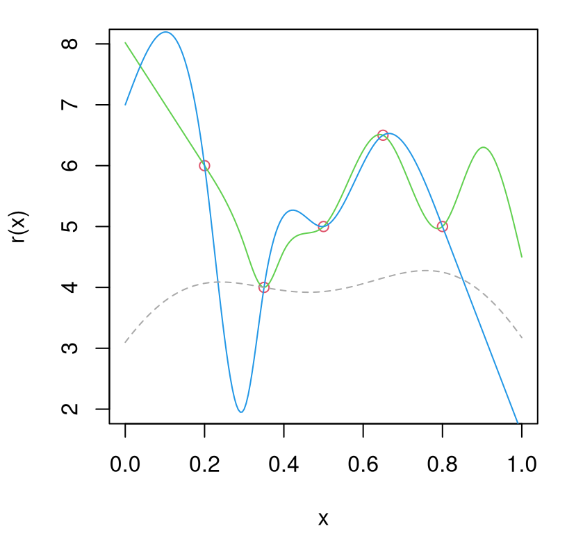
FIGURE 10.9: Variance hypotheses from Figure 10.7 with replicating threshold added in gray.
That green hypothesis is, of course, just one instance of a variance function above the replication threshold. Although those hypotheses were not derived from GP predictive equations, the example illustrates potential. So here’s what we know: replication is 1) good for GP calculations (\(n^3 \ll N^3\)); 2) preferred by IMSPE under certain (changing) variance regimes; and 3) intuitively helps separate signal from noise. But how often is IMSPE going to ask for replications in practice? The short answer: not often enough.
One challenge is numerical precision in optimization when mixing discrete and continuous search. Given a continuum of potential new locations, up to floating-point precision, a particular setting corresponding to a finite number of replicate sites is not likely to be preferred over all other settings, such as ones infinitesimally nearby. Another issue, which is more fundamental, is that IMSPE is myopic. Value realized by the current selection, be it a replicate or new unique location, is not assessed through its impact on a future decision landscape.
10.3.2 Lookahead over replication
Entertaining acquisition decision spaces that are forward looking is hard. Several examples may be found in the literature, primarily emphasizing BO applications (Chapter 7). (See, e.g., David Ginsbourger and Le Riche 2010; Gonzalez, Osborne, and Lawrence 2016; Lam, Willcox, and Wolpert 2016; Huan and Marzouk 2016.) To my knowledge, closed form solutions only exist for the one-step-ahead case. Many approaches, like IECI from §7.2.3, leverage numerics to a degree. More on optimization is provided, in brief, in §10.3.4. In the context of IMSPE, Binois et al. (2019) found that a replication-biased lookahead, correcting myopia in the context of separating signal from noise, is manageable.
Consider a horizon \(h\) into the future, over which the goal is to plan for up to one new, unique site \(\bar{x}_{n+1}\), and \(h\) or \(h+1\) replicates, each at \(n\) or \(n+1\) existing unique locations. The first can be a new, unique site, and the remaining \(h\) replicates. Or replicates can come first, with \(h\) ways to assign a new unique site later. Figure 10.10 provides a flow diagram corresponding to horizon \(h=3\) case. Each node in the graph represents a lookahead state. Red arrows denote potential timings for a new unique site graphically, as a transition between states. Replicates are indicated by black arrows.
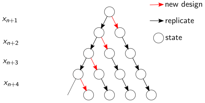
FIGURE 10.10: Flow chart of lookahead over replication. A similar chart may be found in Binois et al. (2019).
Finding each new unique location involves a continuous, potentially derivative-based IMSPE search. Entertaining replicates is discrete. In total, looking ahead over horizon \(h\) requires \(h+1\) continuous searches, and \((h+1)(h+2)/2 -1\) discrete ones. Searching over discrete alternatives, involving replicates at one of the existing \(\bar{x}_k\) locations, \(k=1,\dots,n, n+1\), may utilize a simplified IMSPE (10.9) calculation:
\[\begin{align} I_{n+1}(\bar{x}_k) &= \nu( 1 - \mathrm{tr}(B_k' W_n)), \quad \mbox{ with } \tag{10.13} \\ B_k' &= \frac{\left(\left(C_n + A_n^{-1}\Lambda_n\right)^{-1}\right)_{.,k} \left(\left(C_n + A_n^{-1}\Lambda_n\right)^{-1}\right)_{k,.} }{a_k (a_k + 1)/\lambda_k - \left(C_n + A_n^{-1}\Lambda_n \right)^{-1}_{k,k}}. \notag \end{align}\]
Implementation in hetGP considers \(h \in \{0, 1, 2, \ldots \}\) with \(h=0\) representing ordinary myopic IMSPE search. Although larger values of \(h\) entertain future sequential design decisions, the goal (for any \(h\)) is to determine what to do now as \(N \rightarrow N+1\). Toward that end, \(h+1\) decision paths are entertained spanning alternatives between exploring sooner and replicating later, or vice versa. During each iteration along a given path through Figure 10.10, either Eq. (10.9) or (10.13), but not simultaneously, is taken up as the hypothetical action. In the first iteration, if a new \(\bar{x}_{n+1}\) is chosen by optimizing Eq. (10.9), that location is combined with existing \((\bar{x}_1, \dots, \bar{x}_n)\) and considered as candidates for future replication over the remaining \(h\) lookahead iterations (when \(h \geq 1\)). If instead a replicate is chosen in the first iteration, the lookahead scheme recursively searches over choices of which of the remaining \(h\) iterations will pick a new \(\bar{x}_{n+1}\), with others optimizing over replicates. Recursion is resolved by moving to the second iteration and again splitting the decision path into a choice between replicate-explore-replicate-… and replicate-replicate-…, etc. After fully unrolling the recursion in this way, optimizing up to horizon \(h\) along \(h+1\) paths, the ultimate IMSPE for the respective hypothetical design with size \(N + 1 +h\) is computed, and the decision path yielding the smallest IMSPE is stored. Selection \(x_{N+1}\) is a new location if the explore-first path was optimal, and is a replicate otherwise.
Horizon is a tuning parameter. It determines the extent to which replicates are entertained in lookahead, and therefore larger \(h\) somewhat inflates chances for replication. As \(h\) grows there are more decision paths that delay exploration to a later iteration; if any of them yield smaller IMSPE than the explore-first path, the immediate action is to replicate. Although larger \(h\) allows more replication before committing to a new, unique \(\bar{x}_{n+1}\), it also magnifies the value of an \(\bar{x}_{n+1}\) chosen in the first iteration, as that location could potentially accrue its own replicates in subsequent lookahead or real design iterations. Therefore, although in practice larger \(h\) leads to more replication in the final design, this association is weak.
Before considering criteria for how to set horizon, consider the following illustration with fixed \(h=5\). Take \(f(x) = (6x -2)^2 \sin(12x-4)\) from Forrester, Sobester, and Keane (2008), implemented as f1d in hetGP, and observe \(Y(x)\sim \mathcal{N}(f(x), r(x))\), where the noise variance function is \(r(x) = (1.1 + \sin(2 \pi x))^2\).
This example was engineered to be similar to the motorcycle accident data (§10.2), but allow for bespoke evaluation. Begin with an initial uniform design of size \(N=n=10\), i.e., without replicates, and associated hetGP fit based on a Gaussian kernel.
Using that fit, calculate IMSPE with horizon \(h=5\) lookahead over replication. The IMSPE_optim call below leverages closed form IMSPE (10.11) and derivatives using an optim call with method="L-BFGS-B", mixed with discrete evaluations (10.13).
##  [1] 0.0000 0.1111 0.2222 0.3333 0.4444 0.5556 0.6667 0.7778 0.8889
## [10] 1.0000 0.1710
Whether or not the chosen location, in position eleven above (0.171), is a replicate depends on the random Rmarkdown build, challenging precise narrative here. The hetGP package provides an efficient partitioned inverse-based updating method (6.8), utilizing \(\mathcal{O}(n^2)\) or \(\mathcal{O}(n)\) updating calculations for new data points depending on whether that point is unique or a replicate, respectively. Details are provided by Binois et al. (2019), extending those from §6.3 to the heteroskedastic case.
That’s the basic idea. Let’s continue and gather a total of 500 samples in this way, in order to explore the aggregate nature of sequential design. Periodically, every 25 iterations in the code below, it can help to restart MLE calculations to “unstick” any solutions found in local modes of the likelihood surface. Gathering 500 points is overkill for this simple 1d problem, but it helps create a nice visualization.
for(i in 1:489) {
## find the next point and update
opt <- IMSPE_optim(mod, h=5)
X <- c(X, opt$par)
ynew <- fY(opt$par)
Y <- c(Y, ynew)
mod <- update(mod, Xnew=opt$par, Znew=ynew, ginit=mod$g*1.01)
## periodically attempt a restart to try to escape local modes
if(i %% 25 == 0){
mod2 <- mleHetGP(X=list(X0=mod$X0, Z0=mod$Z0, mult=mod$mult), Z=mod$Z,
lower=0.0001, upper=1)
if(mod2$ll > mod$ll) mod <- mod2
}
}
nrow(mod$X0)## [1] 70Of the \(N=500\) total acquisitions, the final design contains \(n= 70\) unique locations. To help visualize and assess the quality of the final surface with that design, the code below gathers predictive quantities on a dense grid in the input space.
Figure 10.11 shows the resulting predictive surface in red, with true analog in black. Gray vertical bars help visualize relative degrees of replication at each unique input location.
plot(xgrid, f1d(xgrid), type="l", xlab="x", ylab="y", ylim=c(-8,18))
lines(xgrid, qnorm(0.05, f1d(xgrid), fr(xgrid)), col=1, lty=2)
lines(xgrid, qnorm(0.95, f1d(xgrid), fr(xgrid)), col=1, lty=2)
points(X, Y)
segments(mod$X0, rep(0, nrow(mod$X0)) - 8, mod$X0,
  (mod$mult - 8)*0.5, col="gray")
lines(xgrid, p$mean, col=2)
lines(xgrid, qnorm(0.05, p$mean, sqrt(pvar)), col=2, lty=2)
lines(xgrid, qnorm(0.95, p$mean, sqrt(pvar)), col=2, lty=2)
legend("top", c("truth", "estimate"), col=1:2, lty=1)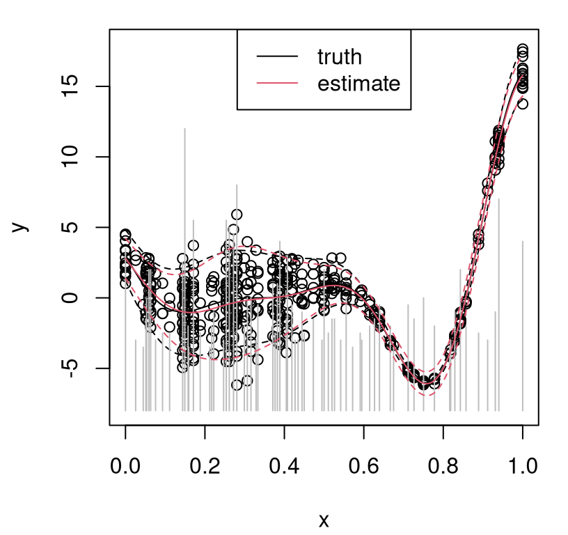
FIGURE 10.11: Sequential design with horizon \(h=5\): truth in black; predictive in red; vertical gray line segments indicate relative degrees of replication.
Both degree of replication and density of unique elements is higher in the high-noise region than where noise is lower. In a batch design setting and in the unique situation where relative noise levels are somehow known, a rule of thumb of more samples or replicates in higher noise regimes is sensible. Such knowledge is unrealistic, and even so the optimal density differentials and degrees of replication aren’t immediate. Proceeding sequentially allows learning to adapt to design and vice versa.
A one-dimensional input case is highly specialized. In higher dimension, where volumes are harder to fill, a more delicate balance may need to be struck between the value of information in high- versus low-noise regions. Given the choice between high- and low-noise locations, which are otherwise equivalent, a low-noise acquisition is clearly preferred. Determining an appropriate lookahead horizon can be crucial to making such trade-offs.
Tuning the horizon
Horizon \(h=5\) is rather arbitrary. Although it’s difficult to speculate on details regarding the quality of the surface presented in Figure 10.11, due to the random nature of the Rmarkdown build, scope for improvement may be apparent. Chances are that uncertainty is overestimated in some regions and underestimated in others. In the version I’m looking at, the right-hand/low-noise region is over-sampled. A solution lies in tuning lookahead horizon \(h\) online. Binois et al. (2019) proposed two simple schemes. The first adjusts \(h\) in order to target a desired ratio \(\rho = n/N\) and thus manage surrogate modeling computational cost through the Woodbury trick (§10.1.1):
\[ \mbox{Target:} \quad h_{N+1} \leftarrow \left\{ \begin{array}{lll} h_N + 1 & \mbox{if } n/N > \rho & \mbox{and a new $\bar{x}_{n+1}$ is chosen} \\ \max\{h_N-1,-1\} & \mbox{if } n/N < \rho & \mbox{and a replicate is chosen} \\ h_N & \mbox{otherwise}. \end{array} \right. \]
Horizon \(h\) is nudged downward when the empirical degree of replication is lower than the desired ratio; or vice versa.12 The second scheme attempts to adapt and minimize IMSPE regardless of computational cost:
\[ \mbox{Adapt:} \quad h_{N+1} \sim \mathrm{Unif} \{ a'_1, \dots, a'_n \} \quad \text{ with }\quad a'_i := \max(0, a_i^* - a_i). \]
Ideal replicate values
\[\begin{equation} a_i^* \propto \sqrt{ r(\bar{x}_i) (K_n^{-1} W_n K_n^{-1})_{i,i}} \tag{10.14} \end{equation}\]
come from a criterion in the SK literature (Ankenman, Nelson, and Staum 2010). See allocate_mult in hetGP and homework exercises in §10.4 for more details. Here the idea is to stochastically nudge empirical replication toward an optimal setting derived by fixing unique-\(n\) locations \(\bar{x}_1,\dots,\bar{x}_n\), and allocating any remaining design budget entirely to replication. An alternative, deterministic analog, could be \(h_{N + 1} = \max_i a_i'\).
Code below duplicates the example above with the adapt heuristic. Alternatively, horizon calls can be provided target and previous_ratio arguments in order to implement the target heuristic instead. Begin by reinitializing the design.
Next, loop to obtain \(N=500\) observations under an adaptive horizon scheme.
for(i in 1:490) {

  ## adaptively adjust the lookahead horizon
  h[i] <- horizon(mod.a)

  ## find the next point and update
  opt <- IMSPE_optim(mod.a, h=h[i])
  X <- c(X, opt$par)
  ynew <- fY(opt$par)
  Y <- c(Y, ynew)
  mod.a <- update(mod.a, Xnew=opt$par, Znew=ynew, ginit=mod.a$g*1.01)

  ## periodically attempt a restart to try to escape local modes
  if(i %% 25 == 0){
    mod2 <- mleHetGP(X=list(X0=mod.a$X0, Z0=mod.a$Z0, mult=mod.a$mult),
      Z=mod.a$Z, lower=0.0001, upper=1)
    if(mod2$ll > mod.a$ll) mod.a <- mod2
  }
}
Once that’s done, predict on the grid.
The left panel of Figure 10.12 shows adaptively selected horizon over iterations of sequential design. Observe that a horizon of \(h=5\) is not totally uncommon, but is also higher than typically preferred by the adaptive scheme. In total, \(n=\) 107 unique sites were chosen – more than in the fixed \(h=5\) case, but in the same ballpark compared to the full size of \(N=500\) acquisitions. The right panel of the figure shows the final design and predictions versus the truth, matching closely that of Figure 10.11 corresponding to the fixed horizon (\(h=5\)) case.
par(mfrow = c(1,2))
plot(h, main="horizon", xlab="iteration")
plot(xgrid, f1d(xgrid), type="l", xlab="x", ylab="y",
  main="adaptive horizon design", ylim=c(-8,18))
lines(xgrid, qnorm(0.05, f1d(xgrid), fr(xgrid)), col=1, lty=2)
lines(xgrid, qnorm(0.95, f1d(xgrid), fr(xgrid)), col=1, lty=2)
points(X, Y)
segments(mod$X0, rep(0,nrow(mod$X0)) - 8, mod$X0,
  (mod$mult - 8)*0.5,  col="gray")
lines(xgrid, p$mean, col=2)
lines(xgrid, qnorm(0.05, p$mean, sqrt(pvar.a)), col=2, lty=2)
lines(xgrid, qnorm(0.95, p$mean, sqrt(pvar.a)), col=2, lty=2)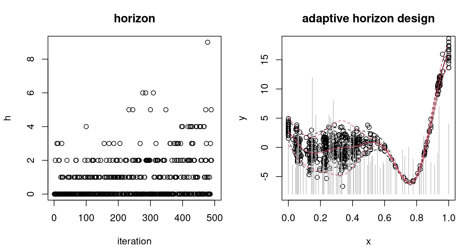
FIGURE 10.12: Horizons chosen per iteration (left); final design and predictions versus the truth (right) as in Figure 10.11.
The code below offers an out-of-sample comparison with RMSE (lower is better).
##      h5      ha
## 0.02014 0.02128
Although it varies somewhat from one Rmarkdown build to the next, a typical outcome is that the adaptive scheme yields slightly lower RMSE. Being able to adjust lookahead horizon enables the adaptive scheme to better balance exploration versus replication in order to efficiently learn a smoothly changing signal-to-noise ratio exhibited by the data-generating mechanism.
10.3.3 Examples
Here we revisit SIR and ATO examples from §10.2.2 from a sequential design perspective.
Susceptible, infected, recovered
Begin with a limited seed design of just twenty unique locations \(n\) and five replicates upon each for \(N=100\) total runs.
X <- randomLHS(20, 2)
X <- rbind(X, matrix(rep(t(X), 4), ncol=2, byrow=TRUE))
Y <- apply(X, 1, sirEval)
A fit to that initial data uses options similar to the batch fit from §10.2.2, augmenting with a fixed mean and limits on \(\theta_{(\delta)}\). Neither is essential in this illustration, but help to limit sensitivity to a small seed design in this random Rmarkdown build.
fit <- mleHetGP(X, Y, covtype="Matern5_2", settings=list(linkThetas="none"),
  known=list(beta0=0), noiseControl=list(upperTheta_g=c(1,1)))
To visualize predictive surfaces and progress over acquisitions out-of-sample, R code below completes the 2d testing input grid XX from the batch example in §10.2.2 with output evaluations for benchmarking via RMSE and score.
Code below then allocates storage for RMSEs, scores and horizons, for a total of 900 acquisitions.
The acquisition sequence here, under an adaptive horizon scheme, looks very similar to our previous examples, modulo a few subtle changes. When reinitializing MLE calculations, for example, notice that fit$used_args is used below to maintain consistency in search parameters and modeling choices.
for(i in 101:N) {

  ## find the next point and update
  h[i] <- horizon(fit)
  opt <- IMSPE_optim(fit, h=h[i])
  ynew <- sirEval(opt$par)
  fit <- update(fit, Xnew=opt$par, Znew=ynew, ginit=fit$g*1.01)

  ## periodically attempt a restart to try to escape local modes
  if(i %% 25 == 0){
    fit2 <- mleHetGP(X=list(X0=fit$X0, Z0=fit$Z0, mult=fit$mult), Z=fit$Z,
      maxit=1e4, upper=fit$used_args$upper, lower=fit$used_args$lower,
      covtype=fit$covtype, settings=fit$used_args$settings,
      noiseControl=fit$used_args$noiseControl)
    if(fit2$ll > fit$ll) fit <- fit2
  }

  ## track progress
  p <- predict(fit, XX)
  var <- p$sd2 + p$nugs
  rmse[i] <- sqrt(mean((YY - p$mean)^2))
  score[i] <- mean(-(YY - p$mean)^2/var - log(var))
}
Figure 10.13 shows the resulting predictive surfaces and design selections. Compare to Figure 10.4 for a batch version. Similarity in these surfaces is high, especially for the mean (left panel), despite an order of magnitude smaller sequential design compared to the batch analog, which was based on more than ten thousand runs. Depending on the random Rmarkdown build, the standard deviation (right) may mis-locate the area of high noise in the \(I_0\) direction, over-sampling in the upper-right corner. This is eventually resolved with more active learning.
par(mfrow=c(1,2))
xx <- seq(0, 1, length=100)
image(xx, xx, matrix(p$mean, ncol=100), xlab="S0", ylab="I0",
  col=cols, main="mean infected")
text(fit$X0, labels=fit$mult, cex=0.5)
image(xx, xx, matrix(sqrt(var), ncol=100), xlab="S0", ylab="I0",
  col=cols, main="sd infected")
text(fit$X0, labels=fit$mult, cex=0.5)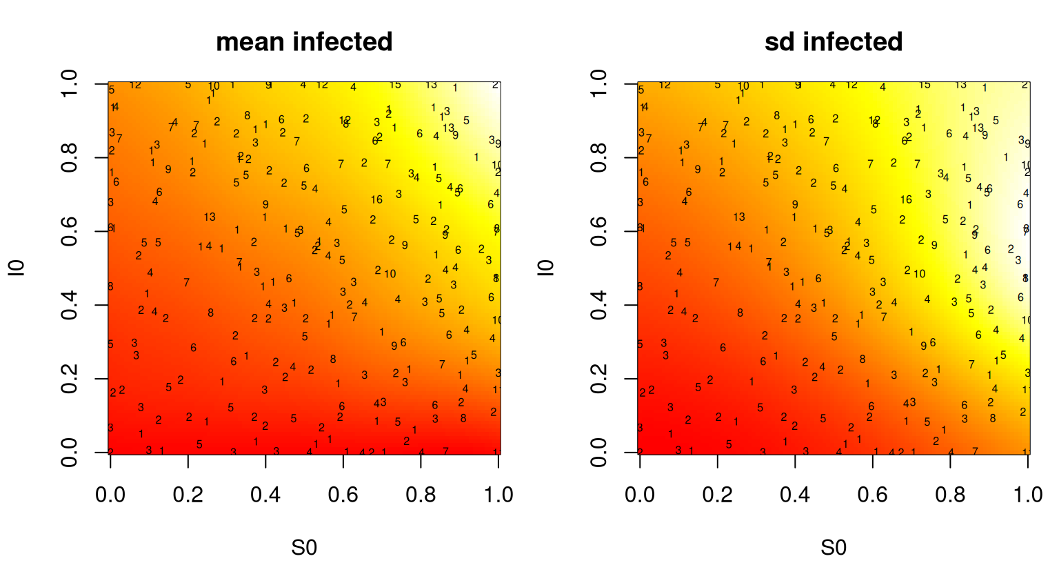
FIGURE 10.13: Heteroskedastic GP fit to sequentially designed SIR data showing predictive mean surface (left) and estimated standard deviation (right). Compare to batch analog in Figure 10.4.
Density of unique locations, indicated by the coordinates of the numbers plotted in both panels, appears uniform to the naked eye. However, degree of replication is greater in the right-half of inputs corresponding to \(S_0 > 0.5\) under the adaptive horizon IMSPE scheme. All double-digit multiplicities are in this right-hand half-plane. As a summary of progress over sequential design iterations, Figure 10.14 shows a progression of RMSEs (left), proper scores (middle) and horizon (right). The first two panels have the batch analog overlayed in dashed-red.
par(mfrow=c(1,3))
plot(rmse, type="l", xlab="n: sequential iterate", ylim=c(0.06, 0.07))
abline(h=sqrt(mean((YY - psir$mean)^2)), col=2, lty=2)
legend("topright", c("sequential", "batch"), col=1:2, lty=1:2)
plot(score, type="l", xlab="n: sequential iterate", ylim=c(4, 5))
abline(h=mean(-(YY - psir$mean)^2/vsir - log(vsir)), col=2, lty=2)
plot(h, xlab="n: sequential iterate", ylab="lookahead horizon")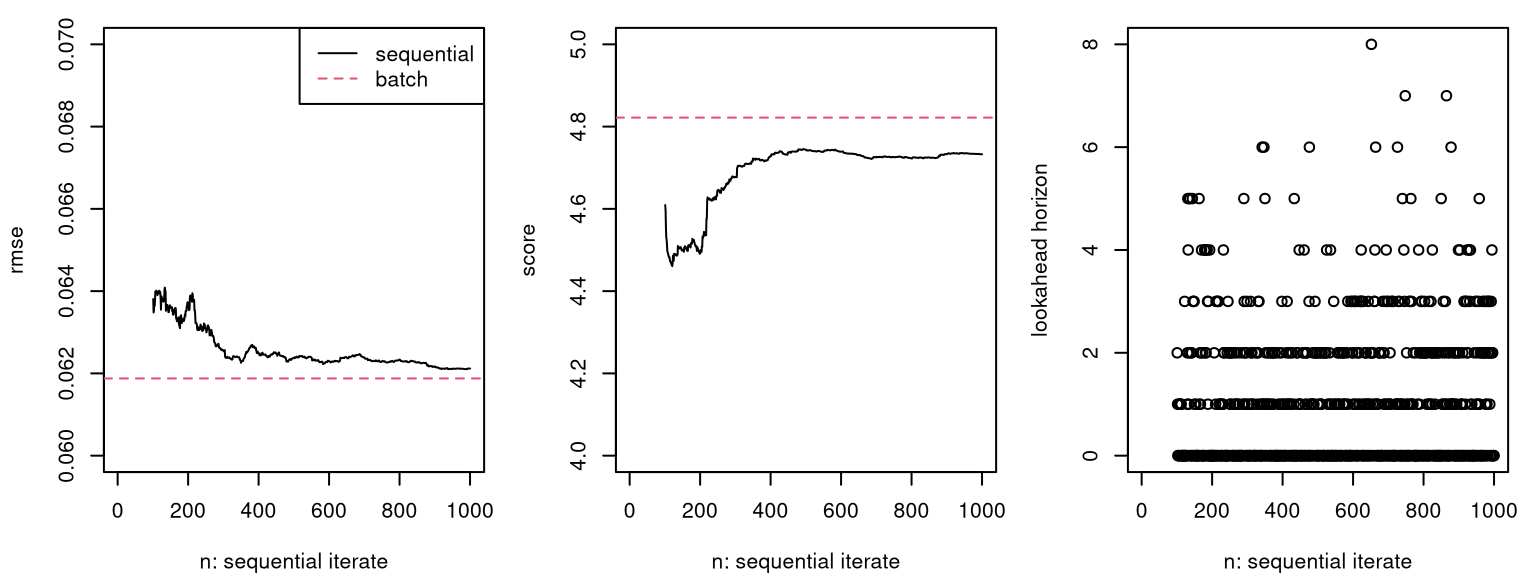
FIGURE 10.14: Summary of sequential design progress via RMSE (left), proper score (middle) and selected lookahead horizon (right) under the adapt scheme.
In spite of the much larger batch training set, our sequential design performs very similarly out-of-sample. Note that both solid and dashed lines depend on random initializations/designs and responses through sirEval. Thus they have a distribution that could be averaged-over in a MC fashion. That exercise is left to the curious reader. To wrap up, observe in the right-hand panel that horizon favors low numbers, emphasizing \(h=0\) and \(h=1\), but more than twenty percent of selections are larger than that.
## [1] 0.2822Limited lookahead horizon is deemed to be beneficial for separating signal from noise in this example. It’s worth reiterating that the IMSPE criterion (10.9) and lookahead horizon (10.14) emphasize mean-accuracy not variance accuracy or minimization. Nevertheless they perform well on score which combines measurements of both. This is because they – especially longer horizons – encourage replication which offers a pure look at noise in order to pin down local variance.
Inventory management
ATO is a much larger example. §10.2.2 leveraged a fit stored in the ato data object. Fitting live in Rmarkdown would’ve represented a prohibitive undertaking. That same data object contains a "hetGP"-class model out.a that was trained under an adaptive horizon IMSPE-based sequential design scheme. The size of that design and the time it took to train are quoted by the output of the code below.
##            n            N time.elapsed
##         1194         2000        38738
Recall that the earlier experiment used \(n=1000\) unique sites with an average of five replicates upon each, for a total of about \(N\approx 5000\) training data points. The actively selected training set here is much smaller, having \(N=2000\) at \(n=\) 1194 unique locations. So the sequential design has more unique locations but still a nontrivial degree of replication, resulting in many fewer overall runs of the ATO simulator. Utilizing the same out-of-sample testing set from the previous score-based comparison, code below calculates predictions and pointwise scores with this new sequential design.
phet.a <- predict(out.a, Xtest)
phets2.a <- phet.a$sd2 + phet.a$nugs
mhet.a <- as.numeric(t(matrix(rep(phet.a$mean, 10), ncol=10)))
s2het.a <- as.numeric(t(matrix(rep(phets2.a, 10), ncol=10)))
sehet.a <- (unlist(t(Ztest)) - mhet.a)^2
sc.a <- - sehet.a/s2het.a - log(s2het.a)
c(batch=mean(sc), adaptive=mean(sc.a))
## batch adaptive
## 3.396 3.616So active learning leads to a more accurate predictor than the earlier batch alternative, despite the former having been trained on about 60% fewer runs. Illustrating those acquisitions requires “rebuilding” the out.a object. To keep hetGP compact for CRAN, \(\mathcal{O}(n^2)\) covariance matrices and inverses have been deleted by providing return.matrices=FALSE to the mleHetGP command used to build out.a.
The calculation sequence for acquisitions involved in this sequential design begins by determining the horizon, and then searching with IMSPE while looking ahead over that horizon. In code, that amounts to the following:
Wijs <- Wij(out.a$X0, theta=out.a$theta, type=out.a$covtype)
h <- horizon(out.a, Wijs=Wijs)
control <- list(tol_dist=1e-4, tol_diff=1e-4, multi.start=30)
opt <- IMSPE_optim(out.a, h, Wijs=Wijs, control=control)
Pre-calculating Wijs (\(W\)) economizes a little on execution time since these are needed by both horizon and IMSPE_optim. A control argument to IMSPE_optim allows users to fine-tune fidelity of search over the criterion. Above, the number of restarts and tolerances on distance to existing sites (i.e., replicates) in search is adjusted upwards of their default settings. For restarts, our adjustments to the default are intended to make search more global. Regarding tolerances, higher values make selection of replicates more likely, determining that optim outputs within 1e-4 of input \(x\) or output \(I_{N+1}(x)\) should snap to existing sites.
##        [,1]   [,2]   [,3]   [,4]    [,5]    [,6]   [,7]   [,8]
## [1,] 0.3492 0.5026 0.4658 0.1668 0.05677 0.07768 0.4406 0.8267
Acquisition is completed by feeding that 8d location into the ATO simulator. Subsequently, the chosen input–output pair would be used to update the model fit. An indication of whether or not the new location is unique (i.e., actually new) or a replicate is provided by the path field in IMSPE_optim output. The path list contains the best sequence of points via elements par, value, and new of the acquisition followed by \(h\) others computed as lookahead selections.
## [1] TRUEATO inputs are actually on a grid, so evaluation would require “snapping” this continuous solution to that grid after undoing any coding of inputs. Further replication could be induced as part of that discretization process.
10.3.4 Optimization, level sets, calibration and more
Throughout this chapter we’ve focused on reducing mean-squared prediction error, a global criterion. Targeting specific regions of interest, such as global minima (BO; Chapter 7) or level sets is also of interest. Bogunovic et al. (2016) provide a treatment unifying criteria for these settings. Consider BO first, having already treated the noisy case in §7.2.4. Picheny, Wagner, and Ginsbourger (2012) provide an important set of benchmarks specifically for this setting. Although there are many suitable criteria for BO with GPs, expected improvement (EI) emerges as perhaps the most appealing because it organically balances exploitation and exploration without any tuning parameters, doesn’t require numerical approximation, and has a closed-form derivative. In the face of noise, and particularly heteroskedasticity, simplicity and computational tractability are important features when adapting a method originally designed for noiseless/deterministic settings.
As mentioned in the lead-in to §10.3.2, lookahead versions of EI have been studied (see, e.g., David Ginsbourger and Le Riche 2010; Gonzalez, Osborne, and Lawrence 2016; Lam, Willcox, and Wolpert 2016; Huan and Marzouk 2016), but closed-form expressions exist only for one-step-ahead versions. Unlike IMPSE, future values of the criterion depend on future function evaluations. Inspired by Lam, Willcox, and Wolpert (2016) and IMSPE-based lookahead presented in §10.3.2, Binois and Gramacy (2018) introduce a replication-biased lookahead for EI which circumvents unknown future function values through simple imputation: \(y_{N+1} \leftarrow \mu_N(x_{N+1})\), which is also known as a kriging “believer” approach (D. Ginsbourger, Le Riche, and Carraro 2010). Examples are left to Section 4.1 in that paper, which is also available as a vignette in the hetGP package.
Active learning for the related problem of contour finding, or level set estimation, proceeds similarly. The objective is to identify a region of inputs defined by a threshold on outputs
\[ \Gamma = \left\{x \in \mathbb{R}^m : Y(x) > T \right\}, \]
where \(T\) can be zero without loss of generality. As with EI, the canonical development is for deterministic settings. In the presence of noise, take \(Y(x) \equiv F(x)\), the latent random field (§5.3.2) with nugget-free epistemic uncertainty \(\breve{\sigma}(x)\) from Eq. (10.10). Criteria defined by Lyu, Binois, and Ludkovski (2018) are implemented for homoskedastic and heteroskedastic GPs and TPs in hetGP. Several other criteria can be found in the literature (Chevalier et al. 2013; Bogunovic et al. 2016; Azzimonti et al. 2016) with a selection of implementations provided by the KrigInv package (Chevalier et al. 2018; Chevalier, Ginsbourger, and Emery 2014; Chevalier, Picheny, and Ginsbourger 2014) on CRAN.
The simplest criterion for active learning in this context is maximum contour uncertainty (MCU), implemented as crit_MCU in hetGP. MCU is based on local probability of misclassification, namely that the function is incorrectly predicted to be below or above \(T\) (Bichon et al. 2008; Ranjan, Bingham, and Michailidis 2008). A second criterion, contour stepwise uncertainty reduction (cSUR), implemented by crit_cSUR in hetGP, amounts to calculating a one-step-ahead reduction of MCU. A more computationally intensive, but more global alternative entails integrating cSUR over the domain in a manner similar to IMSPE (10.9) for variance reduction or IECI (Gramacy and Lee 2011) for BO (§7.2.3). In practice, the integral is approximated by a finite sum, which is the approach taken by crit_ICU in hetGP. Finally, targeted mean-squared error [tMSE; Picheny et al. (2010)], is provided by crit_tMSE and designed to reduce variance close to the target contour. Again, examples are provided in Section 4.2 of Binois and Gramacy (2018).
As a final topic, consider computer model calibration (§8.1) and inverse problems with a noisy, possibly heteroskedastic simulator. I’m not aware of SK or hetGP-like methodology yet being deployed in this setting, but Fadikar et al. (2018) consider quantile kriging [QK; Plumlee and Tuo (2014)] to good effect. Pairing a massive agent-based epidemiological simulation campaign leveraging social networks and data on an Ebola outbreak in Liberia, Fadikar et al. built a QK surrogate for functional output (counts of infecteds over time) via principal components (Higdon et al. 2008) in order to back out a distribution on simulator tuning parameters most likely to have generated an observed (real) sequence of infecteds. Entertaining alternatives to QK, like hetGP, in Rmarkdown on this specific example are complicated by access to a supercomputer scale simulation capability and MATLAB (rather than R) libraries for working with functional output (Gattiker et al. 2016).
In lieu of that, consider the following setup involving similar features without the complications of functional output, and ready access to simulations. Herbei and Berliner (2014) describe a Feynman-Kac simulator, whose source may be downloaded from GitHub, that models the concentration of a tracer within a given spatial domain. One application is modeling oxygen concentration in a thin water layer deep in the ocean (McKeague et al. 2005). The simulator is stochastic, approximating the solution of an advection–diffusion with MC, and is highly heteroskedastic. There are four real-valued inputs: two spatial coordinates (longitude and latitude) and two diffusion coefficients. Interest is in learning, i.e., inverting, the diffusion coefficients. In the notation of Chapter 8, the spatial coordinates are \(x\) and diffusion coefficients are calibration parameters \(u\). So the goal is to use the simulator \(Y^M(x,u)\) to learn \(\hat{u}\) from measurements \(Y^F(x)\) of oxygen concentration in the field, e.g., at \(x\)’s in the Southern Ocean.
In some regions of the input space the simulator response is multimodal, i.e., non-Gaussian, but this can be resolved through minimal (and automatic) replication and averaging. While simulation code is available for C/CUDA, R and MATLAB on the GitHub page, code linked from the book web page provides the essentials; see fksim.R and configuration files fkset.RData read therein, with several enhancements. Coded inputs and sensible defaults for the diffusion coefficients (calibration parameters \(u\)) promote plug-and-playability; automatic degree-6 replication multiplicity with averaging eliminates multimodality.
With those codes, consider simulations along a longitudinal slice in the input space …
… with visual following in Figure 10.15.

FIGURE 10.15: Simulated oxygen concentration along a slice in longitude, with the other three parameters fixed.
Clear signal is evident in the figure, but also clear input-dependent variance. It seems that a much higher degree of replication would be required to effectively separate signal and noise, at least in some parts of the input space, in addition to more exploration to fill out the 4d study area. Two homework exercises in §10.4 take the curious reader through surrogate modeling, design, and inversion with this simulator. For inversion, calibration methods from §8.1 can be applied. Alternatively the log posterior coded below, provided in order to keep our development here somewhat more self-contained, can be used instead.
library(mvtnorm)
lpost.invert <- function(theta, XF, yF, GP)
 {
  ## input processing and checking
  if(length(theta) != ncol(GP$X0) - ncol(XF) + 1)
    stop("length(theta), ncol(XF), ncol(GP$X0) mismatch")
  u <- theta[-length(theta)]
  s2 <- theta[length(theta)]

  ## prior checking
  if(any(u < 0 | u > 1)) return (-Inf)
  if(s2 < 0) return(-Inf)

  ## derive predictive distribution for XF paired with u
  XFU <- cbind(XF, matrix(rep(u, nrow(XF)), ncol=length(u), byrow=TRUE))
  p <- predict(GP, XFU, xprime=XFU)
  C <- s2*diag(nrow(p$cov)) + (p$cov + t(p$cov))/2

  ## gaussian log density evaluation for yF under that predictive
  return(dmvnorm(yF, p$mean, C, log=TRUE) - log(s2))
 }
Notice that lpost.invert, above, is coded to work with a (possibly homoskedastic) "hetGP"-class object GP. Parameter theta combines diffusion coefficients \(u\), in its first several coordinates, with iid noise variance parameter \(\sigma^2\) in its last coordinate. Implicit in lpost.invert is a uniform prior \(u \sim \mathrm{Unif}(0,1)^{m_u}\) and scale-invariant Jeffreys prior \(\sigma^2 \sim 1/\sigma^2\). Arguments XF and YF are field data pairs \((X_{n_F}, Y_{{n_F}})\), observed under the correct but unknown \(u^\star\). That likelihood could be optimized, or used in a Bayesian analysis after placing priors on \(u\). It measures the surrogate predictive probability density of \(Y_{n_F}\)-values when paired with \(X_{n_F}\) and candidate \(u\)-settings. This is more or less equivalent to Kennedy and O’Hagan’s likelihood (8.3) in the “nobias” case.
10.4 Homework exercises
Prompts below explore hetGP variations, sequential design and replication, and application in a calibration (§8.1) setting.
#1: Latent log variances
In §10.2.1 inferential expressions are developed for \(\Lambda_n\) as a diagonal storing smoothed variances for GP modeling with covariance structure \(\nu (C_N + \Lambda_N)\). Unfortunately, such \(\Lambda_n \mid \Delta_n\) given latent \(\Delta_n\) in Eq. (10.7) can be negative, which is bad for a variance. Describe how the scheme can be adapted to work with log variances instead. Hint: the answer to this question is relatively short, but getting it right requires a careful inspection of likelihood and derivatives.
#2: Compensating for mean nonstationarity
§5.3.3 discussed an equivalence between mean and kernel/covariance characterization for GPs. What happens when you fit hetGP, designed for variance nonstationarity, to data which is homoskedastic but exhibits mean nonstationarity? Consider two examples.
- Begin with our favorite 2d data: \(x_1 \exp(-x_1^2 - x_2^2) + \varepsilon \sim \mathcal{N}(0, 0.1^2)\), where \(x \in [-2,4]^2\). In §9.2.2 we used trees to partition up the input space and focus on the interesting lower-left quadrant. We also used it above in §10.1.2. Train homoskedastic and heteroskedastic separable Gaussian kernel GPs to outputs collected on a design composed of a uniform \(21 \times 21\) grid in the input space, with three replicates on each site. Plot the predictive mean and standard deviation surfaces using a \(101 \times 101\) grid and comment. Compare pointwise proper scores [Gneiting and Raftery (2007), Eq. (27); also see §9.1.3] with testing data simulated on that uniform grid.
- Now investigate a 1d response with a regime shift: \(f(x) = \sin(\pi(10x + 0.5)) + 10 (-1)^{\mathbb{I}(x < 0.5)}\), for \(x \in [0,1]\) and observed under standard normal noise. Train homoskedastic and heteroskedastic separable Gaussian kernel GPs to data observed on a uniform length \(n=30\) grid. Visualize the predictive surfaces on a uniform 100-length testing grid and comment. Compare RMSEs and pointwise proper scores using testing evaluations on that grid.
#3: Optimal replication?
Here the goal is to compare SK’s ideal replication (10.14) numbers \(a_i\) at existing training inputs \(\bar{x}_i\), \(i=1,\dots,n\), with lookahead based IMSPE analogs limited to those same sites.
- Create a uniform design in \([0,1]\) of length \(n=21\) and evaluate five replicates of each under
fYfrom §10.3.2 and fit ahetGPsurface using a Matérn \(\nu=5/2\) kernel. (Otherwise thefit <- mleHetGP(...)defaults are fine.) Obtain predictions on a fine grid in the input space and compare your predicted nuggetspredict(...)$nugsto the truthfr. - Suppose the plan was to gather a total of \(N = 201\) simulations from
fY. You’ve gathered \(n=21\) already, so there are \(N_{\mathrm{rest}} = 180\) more to go. Useallocate_multwithNtot\(=N\) to calculate the optimal \(a_i\), for \(i=1,\dots,n\). - Similarly use
opt <- IMSPE_optim(...)with argumenth =\(N_{\mathrm{rest}}\) candidatesXcand=fit$X0from existing unique sites. Record allopt$path[[j]]$paras selected \(x\) locations and extract from those a multiplicity count, i.e., number of replicates, corresponding to each unique setting. - Plot your results from #a–c on common axes and comment.
#4: Ocean sequential design
Consider the ocean/oxygen simulator introduced in §10.3.4. Here we shall treat only the spatial inputs \(x\), leaving diffusion coefficients \(u\) at their default values.
- Build a design in 2d comprised of \(n=25\) unique LHS (§4.1) locations with twenty replicates on each. Obtain simulation responses at these \(N=500\) sites. Fit heteroskedastic and homoskedastic GPs to these data and provide a visual comparison between the two on a \(100 \times 100\) predictive grid, and on a slice of that grid fixing the latitude input near 80% in coded units. Overlay runs from §10.3.4 on that slice and comment. You might find it helpful, but not essential, to use the following settings in your fit(s).
lower <- rep(0.01, 2)
upper <- rep(30, 2)
covtype <- "Matern5_2"
noiseControl <- list(g_min=1e-6, g_bounds=c(1e-6, 1),
  lowerDelta=log(1e-6))
settings <- list(linkThetas="none", initStrategy="smoothed",
return.hom=TRUE)- Now consider sequential design under the heteroskedastic GP only. Begin with \(n_{\mathrm{init}} = 25\) locations, ideally the same ones from #a, but only four replicates on each so that \(N_{\mathrm{init}} = 100\). Acquire 400 more simulations under an adaptive lookahead IMSPE scheme. At the end, augment your visuals from #a, including horizon over the iterations, and comment. You might find it helpful, but not essential, to utilize the following in your IMSPE searches.
- Finally, repeat #a–b at least ten times and save RMSEs and pointwise proper scores calculated on out-of-sample testing data observed on the predictive grid. (No need to repeat the visuals, just the designs and fits.) Provide boxplots of RMSEs and scores and comment.
#5: Ocean calibration
Data in ocean_field.txt contains \(n_F = N_F = 150\) observations of oxygen concentration at sites in the Southern Ocean matching baseline diffusion coefficients \(u^\star\) encoded in the default fksim formals. See §10.3.4 and #4 for details. Separately, build homoskedastic and heteroskedastic GP surrogates from fksim simulation campaign output provided by ocean_runs.txt combining a 4d LHS of size 500, over latitude and longitude \(x\)-sites and two diffusion coefficients \(u\), with a 2d maximin LHS of \(u\)-values paired with \(X_{n_F}\) from the field data. Ten replicate runs at each location are gathered for a grand total of \(N_M = 6000\) simulations. Use lpost.invert from §10.3.4 in order to sample from a Bayesian posterior distribution of \(u\) and \(\sigma^2\), separately for both surrogates. Compare your posterior distribution(s) for \(u\) with true \(u^\star\)-values.
References
hetGP: Heteroskedastic Gaussian Process Modeling and Sequential Design in R.” Available as a Vignette in the R Package.
hetGP: Heteroskedastic Gaussian Process Modeling and Design Under Replication. https://CRAN.R-project.org/package=hetGP.
KrigInv: An Efficient and User-Friendly Implementation of Batch-Sequential Inversion Strategies Based on Kriging.” Computational Statistics & Data Analysis 71: 1021–34.
KrigInv: Kriging-Based Inversion for Deterministic and Noisy Computer Experiments. https://CRAN.R-project.org/package=KrigInv.
mlegp: Maximum Likelihood Estimates of Gaussian Processes. https://CRAN.R-project.org/package=mlegp.
GLASSES: Relieving the Myopia of Bayesian Optimisation.” In Proceedings of the 19th International Conference on Artificial Intelligence and Statistics, 790–99.
plgp: Particle Learning of Gaussian Processes. https://CRAN.R-project.org/package=plgp.
monomvn: Estimation for Multivariate Normal and Student-\(t\) Data with Monotone Missingness. https://CRAN.R-project.org/package=monomvn.
tgp: Bayesian Treed Gaussian Process Models. https://CRAN.R-project.org/package=tgp.
DiceKriging: Kriging Methods for Computer Experiments. https://CRAN.R-project.org/package=DiceKriging.
Letter \(\nu\) is preferred here to the familiar \(\tau^2\) from Chapter 5 to avoid double squaring: \(\nu^2 \equiv (\tau^2)^2\).↩︎
Horizon \(h=-1\) corresponds a software implementation detail eliminating (setting to zero) thresholds applied to identify as replicates the results of continuous derivative-based searches residing nearby existing \(\bar{x}_k\). Setting these to zero reduces selection of replicates, but doesn’t entirely preclude them since Eq. (10.13) outcomes are still entertained.↩︎