Chapter 4 Space-filling Design

This segment puts the cart before the horse a little. Nonparametric spatial regression, emphasizing Gaussian processes in Chapter 5, benefits from a more agnostic approach to design compared to classical, linear modeling-based, response surface methods. One of the goals here is pragmatic from an organizational perspective: to have some simple, good designs for illustrations and comparisons in later chapters. Designs here are model-free, meaning that we don’t need to know anything about the (Gaussian process) models we intend to use with them, except in the loose sense that those are highly flexible models which impose limited structure on the underlying data they’re trained on. Later in Chapter 6 we’ll develop model-specific analogs and find striking similarity, and in some sense inferiority – a bizarre result considering their optimality – compared to these model-free analogs.

Here we seek so-called space-filling designs, ones which spread out points with the aim of encouraging a diversity of data once responses are observed. A spread of training examples, the thinking goes, will ultimately yield fitted models which smooth/interpolate/extrapolate best, leading to more accurate predictions at out-of-sample testing locations. Our development will focus on variations between, and combinations of, two of the most popular space-filling schemes: Latin hypercube sampling (LHS), and maximin distance designs. Both are based on geometric criteria but offer optimal spread in different senses. LHSs are random, so they disperse in a probabilistic sense, targeting a certain uniformity property. Maximin designs are more deterministic, even if many solvers for such designs deploy stochastic search. They seek spread in terms of relative distance.

Plenty of other model-free, space-filling designs enjoy wide popularity, but they’re mostly variations on a theme. It’s a lot of splitting hairs about subtly different geometric criteria, coupled with vastly different highly customized solving algorithms, producing designs that are visually and practically indistinguishable from one another. The aim here is twofold: 1) to have a nice conceptual base to jump off from, and contrast with the more interesting topic of model-based sequential design (§6.2 and Chapter 7); 2) to have an intuitive default from which to initialize a more ambitious such sequential search.

The entirety of this chapter, and indeed much of the rest of the text, presumes coded inputs in $[0,1]^m$ unless otherwise stated. So the goal is a space-filling design of a desired run size $n$ in the unit hypercube. As an auxiliary consideration, we’ll explore the possibility of “growing” a design to size $n' + n$ from an initial fixed design of size $n$ when additional experimental resources allow augmenting the training dataset. There the goal will be more modest: to best respect, or at least not drastically offend, an underlying space-filling criteria as regards the choice of $n'$ new locations.

4.1 Latin hypercube sample

One simple option for design is random uniform. That is, fill a design matrix $X_n$ in $[0,1]^m$ with $n$ runs via runif.

m <- 2
n <- 10
X <- matrix(runif(n*m), ncol=m)
colnames(X) <- paste0("x", 1:m)

The trouble is, randomness is clumpy. With $n$ of any reasonable size relative to input dimension $m$ you’re almost guaranteed to get design locations right next to one another, and thus gaps in other parts of the input space. Figure 4.1 illustrates this with the single random example generated above.

plot(X, xlim=c(0,1), ylim=c(0,1))

FIGURE 4.1: Random designs can be clumpy.

It can be useful to repeat that example, visualizing new random designs in several replicates. A takeaway from such an exercise is undoubtedly that designs offering reasonable “fill” in the 2d input space are quite rare indeed. Although we don’t bother to describe the formalism, nor undertake calculations to make the following statement precise, it’s not a difficult exercise for one so-inclined. The probability of observing at least two points close to one other, as a relative share of the total input space (with $n = 10$ runs in $m = 2$ input dimensions), is quite high. Therefore the chance of adequately filling the space, at least from an aesthetic perspective, is quite low. Now clumpiness in a design for computer surrogate modeling is not necessarily a bad thing. In fact, purely random designs can be good in some cases (B. Zhang, Cole, and Gramacy 2020). But let’s table that discussion for a moment.

Latin hypercube samples (LHSs) were created, or perhaps borrowed (more details below) from another literature, to alleviate this problem. The goal is to guarantee a certain degree of spread in the design, while otherwise enjoying the properties of a random uniform sample. LHSs accomplish that by divvying the design region evenly into cubes, by partitioning coordinates marginally into equal-sized segments, and ensuring that the sample contains just one point in each such segment. In 2d, which is perhaps over-emphasized due to ease of visualization, the pattern of selected cubes (i.e., those containing a sample) resemble Latin squares.

Since the location of the point within the selected cube is allowed to be random, the LHS doesn’t preclude two points located nearby one another. For example, two points may reside near a corner in common between a cube from an adjacent row and column. This will be easy to see in our visualizations shortly. However the LHS does limit the number of such adjacent cases, guaranteeing a certain amount of spread. But we’re getting ahead of ourselves; how do we construct an LHS? For the description below, I’d like to acknowledge a chapter by Lin and Tang (2015) as a primary source of material for this presentation.

A Latin hypercube (LH) of $n$ runs for $m$ factors is represented by an $n \times m$ matrix $L = (l_{ij})$. Each column $l_j$, for $j=1,\dots,m$, contains a permutation of $n$ equally spaced levels. For convenience, the $n$ levels may be taken to be

\[ -(n-1)/2, -(n-3)/2, \dots, (n-3)/2, (n-1)/2. \]

Right now levels span from $-(n-1)/2$ to $(n-1)/2$, so $L$ spans $[-(n-1)/2, (n-1)/2]^m$. This is a mismatch to our design region $[0,1]$ in $m$ coordinates. But don’t worry – we’ll fix that with a normalization step momentarily.

A Latin hypercube sample (LHS), or sometimes design (LHD), $X_n$ in the design space $[0,1]^m$ is an $n \times m$ matrix with $(i,j)^{\mathrm{th}}$ entry

\[\begin{equation} x_{ij} = \frac{l_{ij} + (n-1)/2 + u_{ij}}{n}, \quad i=1,\dots,n, \; j=1,\dots,m, \tag{4.1} \end{equation}\]

where the $u_{ij}$’s are independent uniform random deviates in $[0,1]$. Observe that the denominator $n$ normalizes so that $x_{ij}$ is mapped into $[0,1]^m$. The $(n-1)/2$ term chooses a point in the corner of the selected square or (hyper) cube. Random adjustments $u_{ij}$ place the $j^{\mathrm{th}}$ coordinate of run $i$ elsewhere in the cube. If instead each $u_{ij}$ is taken to be 0.5 the result is called a Latin sample, which will put $x_{ij}$ right in the middle of one of the squares or (hyper) cubes.

If that verbal description seems complicated, its codification is relatively straightforward. The first step is to create the levels, which depend on the desired number of runs in the design, $n$.

l <- (-(n - 1)/2):((n - 1)/2)

Next, put $m$ randomly permuted versions of the level vector l into a $n \times m$ matrix L.

L <- matrix(NA, nrow=n, ncol=m)
for(j in 1:m) L[,j] <- sample(l, n)

Finally, create a uniform jitter matrix U and combine with the level matrix L following a vectorized version of Eq. (4.1).

U <- matrix(runif(n*m), ncol=m)
X <- (L + (n - 1)/2 + U)/n

What do we get? Figure 4.2 shows the design X as open circles, and uses the vector of levels l to demarcate candidate Latin squares with gray-dashed lines.

plot(X, xlim=c(0,1), ylim=c(0,1), xlab="x1", ylab="x2")
abline(h=c((l + (n - 1)/2)/n,1), col="grey", lty=2)
abline(v=c((l + (n - 1)/2)/n,1), col="grey", lty=2)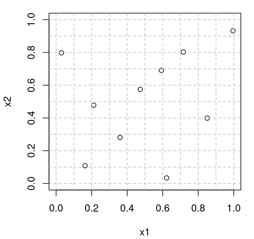

FIGURE 4.2: Latin hypercube sample (LHS) in 2d.

If we were to instead shade the squares containing the dots gray, dropping the dots, we’d have a Latin hypercube; forcing U=1/2 and placing the dot in the middle of the square yields the Latin sample. Both represent useful exercises for the curious reader hoping to gain better insight into what’s going on. Permuting l, comprising columns of L, ensures that each margin, $j \in \{1,2\}$ representing $x_1$ and $x_2$ in this $m=2$ dimensional example, contains just one dot in each segment of the grid in that dimension. Said another way, each column and each row (demarcated by the gray-dashed lines) in the plot has just one dot. Consequently each margin, when projecting over the other input, is uniformly distributed in that coordinate. More detail on these features is provided momentarily, and in greater generality in higher dimension $m$.

But first, let’s write a function that does it so we don’t have to keep cutting-and-pasting the code above. That code is essentially ready-to-go for arbitrary $m \equiv$ m, so all we’re really doing here is wrapping those lines in an R function. Think of this as a more directly useful alternative to the formal boxed environment used elsewhere in the book to demarcate pseudocode for higher-level algorithmics.

mylhs <- function(n, m)
 {
  ## generate the Latin hypercube 
  l <- (-(n - 1)/2):((n - 1)/2)
  L <- matrix(NA, nrow=n, ncol=m)
  for(j in 1:m) L[,j] <- sample(l, n)

  ## draw the random uniforms and turn the hypercube into a sample
  U <- matrix(runif(n*m), ncol=m)
  X <- (L + (n - 1)/2 + U)/n
  colnames(X) <- paste0("x", 1:m)

  ## return the design and the grid it lives on for visualization
  return(list(X=X, g=c((l + (n - 1)/2)/n,1)))
 }

The LHS output resides in the $X field of the list returned. To aid in visualization, grid points are also returned via $g.

4.1.1 LHS properties

When using the new “library routine”, what can be expected in higher dimension $m \equiv$ m? As we noticed in Figure 4.2, LHSs are constructed so that there’s exactly one point in each of the $n$ intervals

\[ [0,1/n), [1/n, 2/n), \dots, [(n-1)/n,1), \]

partitioning up each input coordinate, $j=1, \dots, m$. This property is referred to as one-dimensional uniformity. As a consequence of that property, any projection into lower dimensions that can be obtained by dropping some of the coordinates will also be distributed uniformly. Therefore that lower $m'$-dimensional design will also be an LHS in the $m' < m$ dimensional unit hypercube. This property is perhaps apparent by inspecting the algorithmic description above, or its implementation in code. What happens for a column of L or X is independent of, yet identical to, calculations for other columns.

As an illustration, consider an $m=3$ dimensional LHS with $n = 10$ runs using our library routine.

Dlist <- mylhs(10, 3)

Figure 4.3 shows the first two coordinates of that sample.

plot(Dlist$X[,1:2], xlim=c(0,1), ylim=c(0,1), xlab="x1", ylab="x2")
abline(h=Dlist$g, col="grey", lty=2)
abline(v=Dlist$g, col="grey", lty=2)

FIGURE 4.3: Two-dimensional projection of a 3d LHS.

Observe that this sample is a perfectly good $m=2$ LHS, having only one point in each row and column of the 2d grid, despite being generated in 3d. The other two pairs of inputs show the same property in Figure 4.4. Any of these three (or ${m \choose 2}$ more generally) two-dimensional projections would be a perfectly good 2d LHS.

Is <- as.list(as.data.frame(combn(ncol(Dlist$X),2)))[-1]
par(mfrow=c(1,length(Is)))
for(i in Is) {
  plot(Dlist$X[,i], xlim=c(0,1), ylim=c(0,1), 
    xlab=paste0("x", i[1]), ylab=paste0("x", i[2]))
  abline(h=Dlist$g, col="grey", lty=2)
  abline(v=Dlist$g, col="grey", lty=2)
}

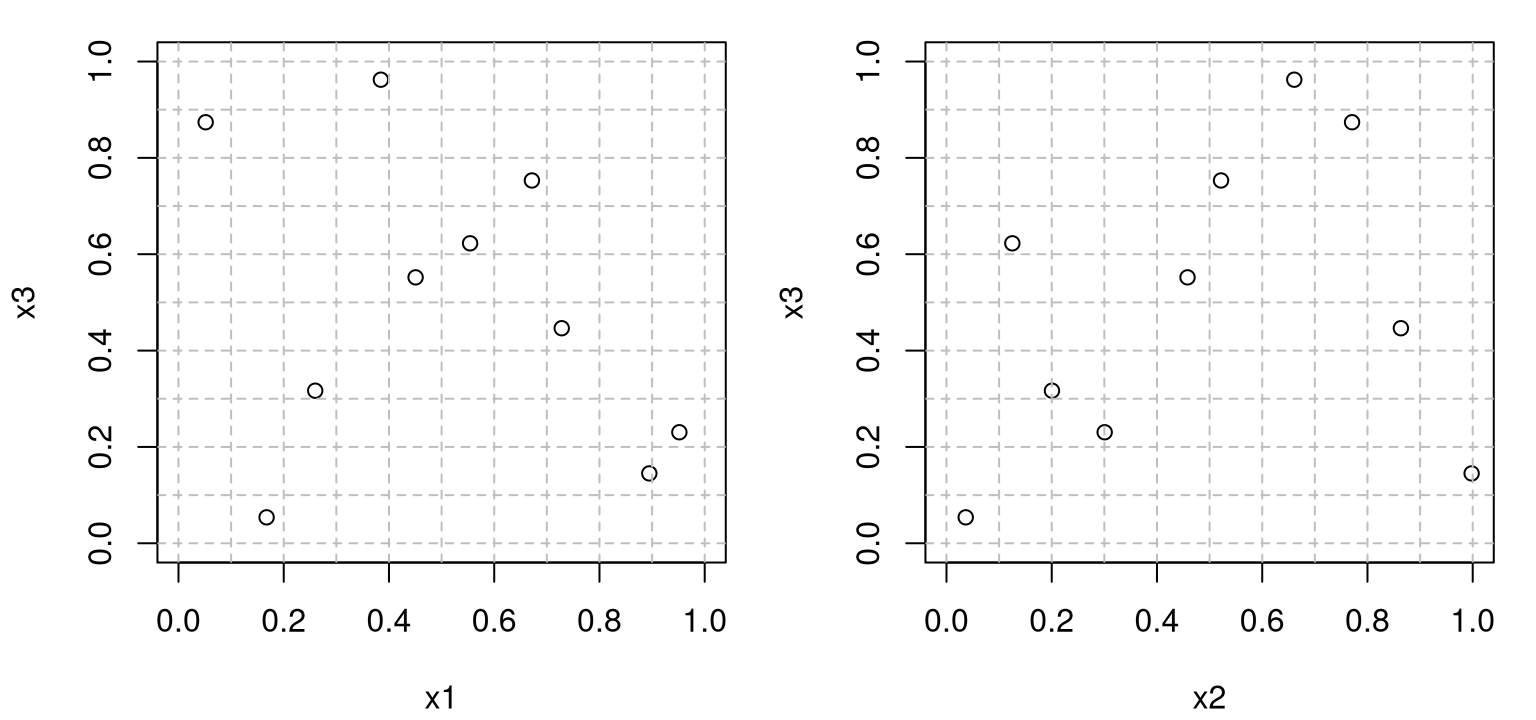
FIGURE 4.4: Remaining pairs of coordinates beyond the one shown in Figure 4.3.

Projecting down into one dimension reveals uniform distributions on the margins. Figure 4.5 utilizes a much larger LHS so that the resulting histograms look more convincingly uniform. An analog using the previous $n=10$ sample, potentially under replication, also provides an instructive suite of visualizations.

X <- mylhs(1000, 3)$X
par(mfrow=c(1,ncol(X)))
for(i in 1:ncol(X)) hist(X[,i], main="", xlab=paste0("x", i))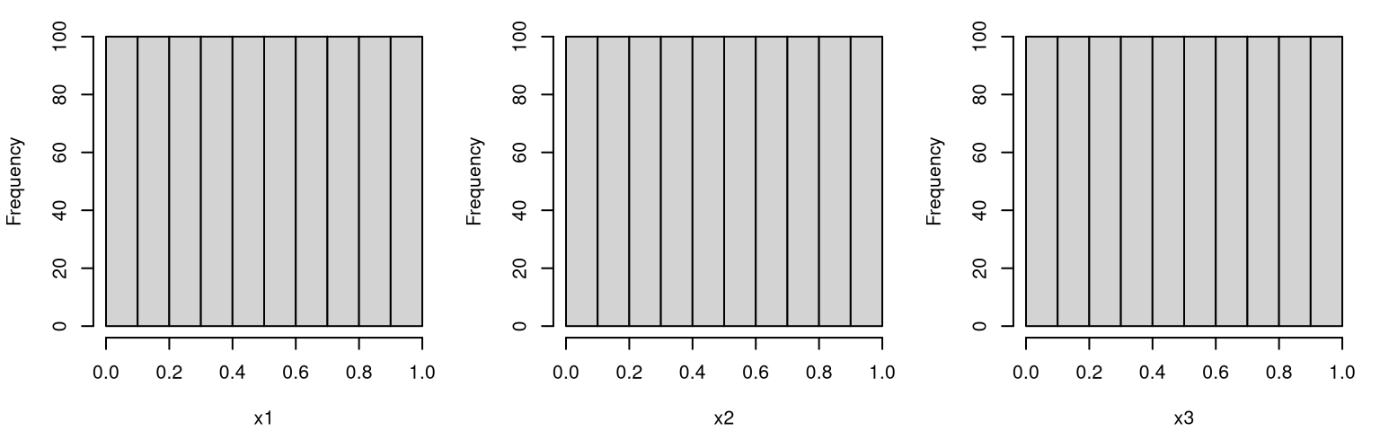

FIGURE 4.5: Histograms of one-dimensional LHS margins.

Popularity of LHSs as designs can largely be attributed to their role in reducing variance in numerical integration. Consider a function $y = f(x)$ where $f$ is known, and $x$ has a uniform distribution on $[0,1]^m$, and where we wish to estimate $\mathbb{E}\{Y\}$ via

\[ \hat{\mu} = \frac{1}{n} \sum_{i=1}^n f(x_i), \quad x_i \stackrel{\mathrm{iid}}{\sim} U[0,1]^m. \]

It turns out that if $f(x)$ is monotone in each coordinate of $x$ then the variance of $\hat{\mu}$ is lower if an LHS is used rather than simple random sampling.

One drawback of LHSs is that, although a degree of space-fillingness is guaranteed at the margins, there’s no guarantee that the resulting design won’t otherwise be somehow aliased, i.e., revealing patterns or clumpiness in other aspects of the variables’ joint distribution. For example, the code chunk below repeatedly draws LHSs with $(n,m)=(10, 2)$, stopping when one is found satisfying a loosely specified monotonicity condition: where the second coordinate is roughly increasing in the first, basically lining up along a jittered diagonal. A counter is used to tally the number of attempts before that criterion is met.

count <- 0
while(1) { 
  count <- count + 1
  Dlist <- mylhs(10, 2)
  o <- order(Dlist$X[,1])
  x <- Dlist$X[o,2]
  if(all(x[1:9] < x[2:10] + 1/20)) break 
}

Figure 4.6 shows the design that caused the code’s execution to break out of the while loop, finding an LHS that met that loose monotonicity criterion.

plot(Dlist$X, xlim=c(0,1), ylim=c(0,1), xlab="x1", ylab="x2")
text(0.2, 0.85, paste("count =", count))
abline(v=Dlist$g, col="grey", lty=2)
abline(h=Dlist$g, col="grey", lty=2)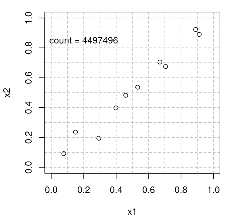

FIGURE 4.6: Potential for aliasing in LHSs.

Clearly this is an undesirable space-filling design in 2d, even though the 1d marginals are nice and uniform. Admittedly, it takes a ton of iterations (approximately 4500 thousand in this run) to find the pattern we were looking for. But that’s one of many patterns out of perhaps an enormous collection of dots that could have yielded an aesthetically undesirable design. Despite many attractive properties, besides being easy to compute, a condition on marginals is a crude way to spread things out, and one which has diminishing returns in increasing dimension. In high dimensions (big $m$ relative to $n$) everything looks like some kind of pattern, so perhaps the distinction between (totally) uniform random and LHSs is academic in that setting.

Suggesting potential remedies will require extra scaffolding which is offered, in part, in §4.2 on maximin design. In the meantime – and to end the LHS description on a high rather than low note – it’s worth discussing several simple-yet-powerful enhancements unique to the LHS setting.

4.1.2 LHS variations and extensions

LHSs may be extended to marginals other than uniform through a simple inverse cumulative distribution function (CDF) transformation. The steps are:

Generate an ordinary LHS, then
apply an inverse CDF (quantile function) of your choice on each of the marginals.

This will cause the marginals to take on distributions with those CDFs, but at the same time ensure that there’s not “more clumpiness than necessary” in the joint distribution. The simplest application of this is to re-scale to a custom hyperrectangle to accommodate another coding of the inputs, or directly in the natural scale.

Again in lieu of a boxed algorithm environment, R code below generalizes our mylhs library routine to utilize beta distributed marginals, of which uniform is a special case. Parameters $\alpha$ and $\beta$ are specified as $m$-vectors shape1 and shape2 following the nomenclature used by qbeta, R’s built-in quantile function for beta distributions. Besides returning a matrix of design elements, the implementation also provides a matrix of beta-mapped grid lines $g. Vector $g no longer suffices since grid elements are now input-coordinate dependent.

mylhs.beta <- function(n, m, shape1, shape2)
 {
  ## generate the Latin Hypercube and turn it into a sample
  l <- (-(n - 1)/2):((n - 1)/2)
  L <- matrix(NA, nrow=n, ncol=m)
  for(j in 1:m) L[,j] <- sample(l, n)
  U <- matrix(runif(n*m), ncol=m)
  X <- (L + (n - 1)/2 + U)/n

  ## calculate the grid for that design
  g <- (L + (n - 1)/2)/n
  g <- rbind(g, 1)

  for(j in 1:m) { ## redistrbute according to beta quantiles
    X[,j] <- qbeta(X[,j], shape1[j], shape2[j])
    g[,j] <- qbeta(g[,j], shape1[j], shape2[j])
  }
  colnames(X) <- paste0("x", 1:m)

  ## return the design and the grid it lives on for visualization
  return(list(X=X, g=g))
}

By way of illustration, consider a 2d LHS with $n=10$ under $\mathrm{Beta}(3, 2)$ and $\mathrm{Beta}(1/2, 1/2)$ marginals.

Dlist <- mylhs.beta(10, 2, shape1=c(3,1/2), shape2=c(2,1/2))

Figure 4.7 shows behavior matching what was prescribed: density of grid locations (and samples) is highest to the right of middle in $x_1$, targeting a mean of $3/(2+3) = 3/5$, and at the edges of the $x_2$ coordinate owing to the “U-shape” of $\mathrm{Beta}(1/2, 1/2)$.

plot(Dlist$X, xlim=c(0,1), ylim=c(0,1), xlab="x1", ylab="x2")
abline(v=Dlist$g[,1], col="grey", lty=2)
abline(h=Dlist$g[,2], col="grey", lty=2)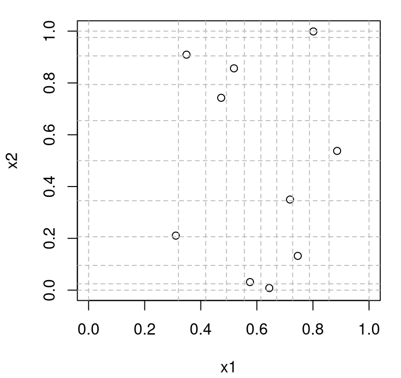

FIGURE 4.7: Two-dimensional LHS with beta marginals.

To look closer at the marginals, code below generates a much larger LHS …

X <- mylhs.beta(1000, 2, shape1=c(3,1/2), shape2=c(2,1/2))$X

… and Figure 4.8 presents histograms of samples obtained in each coordinate against PDF evaluations under the desired beta distributions.

par(mfrow=c(1,2))
x <- seq(0,1,length=100)
hist(X[,1], main="", xlab="x1", freq=FALSE)
lines(x, dbeta(x, 3, 2), col=2)
hist(X[,2], main="", xlab="x2", freq=FALSE)
lines(x, dbeta(x, 1/2, 1/2), col=2)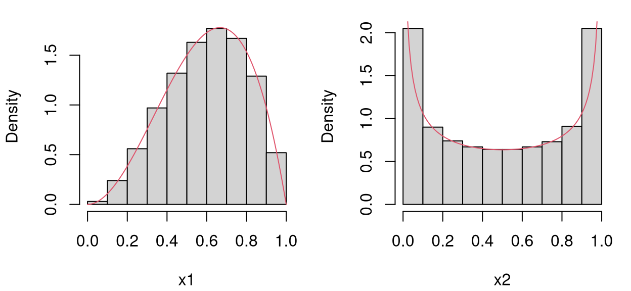

FIGURE 4.8: Marginals of LHS with beta distributions.

Designs generated in this way are useful for input sensitivity analyses, discussed in detail in §8.2, and related exercises common in the uncertainty quantification (UQ) literature. An important aspect in both settings involves exploring how a distribution on inputs propagates to a distribution of outputs through an opaque blackbox apparatus. Random sampling can facilitate a study of main effects and second-order uncertainty indices for nominal inputs under random jitter, or for inputs concentrated in a typical regime. LHSs offer similar functionality while requiring many fewer samples be pushed through a computationally intensive blackbox, say one constructed as a daisy-chain of numerical solvers, surrogates, and so on.

LHSs are also handy in synthetic predictive benchmarking exercises emphasizing assessment of generalization error. Sometimes these are called “bakeoffs” or “horse races”. The idea is to generate training and out-of-sample testing sets where input–output pairs from the former are used to build fitted models of several varieties, and ones from the latter are held out to subsequently compare predictors derived from those fitted models. Inputs from an LHS offer certain guarantees on spread, and when collected simultaneously for training and testing can yield a partition where out-of-sample measurements are made on novel (but not too novel) input settings. Outputs for such exercises could come from any of the synthetic data generating functions offered by the VLSE, for example.

To illustrate, consider the following partition of an $n=20$ LHS in 2d where training inputs come from the first ten, and testing from the last ten.

Dlist <- mylhs(20, 2)
Xtrain <- Dlist$X[1:10,]
Xtest <- Dlist$X[11:20,]

Figure 4.9 visualizes the two sets on the combined LH grid.

plot(Xtrain, xlim=c(0,1), ylim=c(0,1), xlab="x1", ylab="x2")
points(Xtest, pch=20)
abline(v=Dlist$g, col="grey", lty=2)
abline(h=Dlist$g, col="grey", lty=2)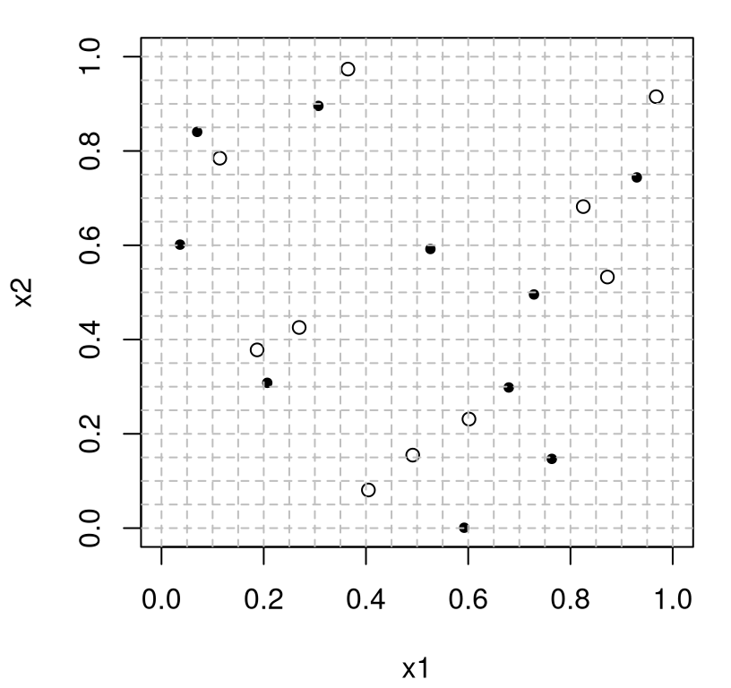

FIGURE 4.9: LHS training and testing partition.

Observe that testing and training locations are spaced out both relative to themselves and to those from the other set. The thinking is that a prediction exercise based upon these inputs would reduce variance in assessments of generalization error, i.e., when measuring the quality of predictions made for inputs somewhat different than ones the fitted models were trained on. It’s common to base horse races or bakeoffs on summaries obtained from repetitions on this theme, as codified by Algorithm 4.1.

Algorithm 4.1: LHS Bakeoff

Assume input dimension $(m)$ is a match for test function $f$, and that the $K$ competing methods are appropriate for $f$.

Require test function $f$, $K$ fitting/prediction methods, training size $n$, testing size $n'$, and number of repetitions $R$.

Repeat the following for $r=1,\dots,R$:

Generate an LHS of size $n+n'$ creating $X$.
Evaluate the true response at all $n+n'$ sites, yielding $Y \sim f(X)$, and combine them with inputs to obtain $n+n'$ data pairs $D = (X, Y)$.
Randomly partition into $n$ training pairs $T_n=(X^t_n, Y^t_n)$ and $n'$ testing or validation pairs $V_{n'} = (X^v_{n'}, Y^v_{n'})$.
- Since rows of the LHS are random, as from mylhs, it’s usually sufficient to take the first $n$ and last $n'$ pairs, respectively.
Train $K$ competing methods on $T_n$ yielding predictors $\hat{y}^{(k)}(\cdot) \equiv \hat{y}^{(k)}(\cdot) \mid T_n$, for $k=1,\dots,K$.
Test out-of-sample by making predictions on the validation set $V_{n'}$, saving them as $\hat{Y}^{(k)}_{n'} = \hat{y}^{(k)}(X^v_{n'})$.
Calculate metrics $m_{r}^{(k)}$ for each method $k=1,\dots,K$ comparing $\hat{Y}^{(k)}_{n'}$ to the held-out values $Y^v_{n'}$. Examples include
- proper scoring rule (See §5.2 and Gneiting and Raftery 2007),
- root mean-squared (prediction) error (RMSE) or mean absolute error (MAE), respectively

\[ \begin{aligned} m_r^{(k)} &= \sqrt{\frac{1}{n'} \sum_{i=1}^{n'} (y_i^v - \hat{y}_i^{(k)})^2}, && \mbox{or} & m_r^{(k)} &= \frac{1}{n'} \sum_{i=1}^{n'} |y_i^v - \hat{y}_i^{(k)}|. \end{aligned} \]

Return one or more $R \times K$ matrices $M$ comprised of $m_r^{(k)}$-values calculated in Step 6, above, and/or more compact summaries of their empirical distribution in order to determine the winner of the bakeoff.

Some notes about typical use follow. Perhaps the most common setting is $n' = n$ so that testing size is commensurate with training. However in situations where computation involved in fitting limits the training size, $n$, but prediction is much faster (i.e., as is the case for GPs in Chapter 5), an $n' \gg n$ setup is sometimes used. It’s typical for $y$-values from $f$ to be observed with noise, e.g., $y = f(x) + \varepsilon$, where $\varepsilon \sim \mathcal{N}(0, \sigma^2)$, yet deterministic settings are common when studying computer experiments. Notation $Y \sim f(X)$ above is intended to cover both cases. Sometimes one is interested in training on noisy data, but making predictive comparisons to de-noised versions, say via RMSE or MAE. This may be implemented with a simple adaptation to the algorithm. However note that proper scores must use a noisy testing set.

One reason to prefer returning a raw $R \times K$ matrix of metric evaluations, $M$, as opposed to a summary (say column-wise averages, quantiles or boxplots), is that the former makes it easier to change your mind later. If the relative comparison turns out to be a “close call”, in terms of average values say, then pairwise $t$-tests (possibly on the log of the metric) can be helpful to adjudicate in order to determine a winner.

But we’re getting a little ahead of ourselves here. We haven’t really introduced any predictors to compare yet, so it’s hard to make things concrete with an example at this time. The curious reader may wish to “fast forward” to a comparison between GP variations and MARS in §5.2.7 styled in the form of Algorithm 4.1.

While the testing set is spread out relative to the training set in the partition in Figure 4.9, these partition elements are not themselves LHSs. That is, they don’t make up a nested LHS (Qian 2009), which might be a desirable property to have. Moreover, unless the plan is to randomize over the partition, as in the GP comparison referenced above, the random nature of an LHS may be undesirable. Or at the very least it’s a double-edged sword: randomization necessitates devoting valuable computational resources to repetition and can lead to insecurities about how much is enough. Many of the drawbacks of LHSs, like that spread is not guaranteed (aliasing is always present to a degree), are a consequence of its inherent randomness. Getting points with maximal spread, whether for one-shot design, train–test partitions, or for sequential analysis, requires swapping a measure of randomization for optimization.

4.2 Maximin designs

If what we want is points spread out, then perhaps it makes sense to design criteria that deliberately spreads points out! For that we need a notion of distance by which to measure spread. The development here takes the simple choice of (squared) Euclidean distance

\[ d(x, x') = ||x - x'||^2 = \sum_{j=1}^m (x_j - x_j')^2, \]

but the framework is otherwise quite general if other choices, such as say Mahalanobis distance, were desired instead. A design $X_n = \{x_1, \dots, x_n\}$ which maximizes the minimum distance between all pairs of points,

\[ X_n = \mathrm{argmax}_{X_n} \min \{ d(x_i, x_k) : i \ne k = 1,\dots, n\}, \]

is called a maximin design.

The opposite way around, so-called minimax designs, also leads to points all spread out. By limiting how far apart pairs of points can be, you end up encouraging spread in a circuitous manner. Many of the considerations are similar, so we won’t get into further detail here on minimax designs. It turns out they’re somewhat harder to calculate than the more conceptually straightforward maximin in practice. See M. Johnson, Moore, and Ylvisaker (1990) for more discussion. Tan (2013) is also an excellent resource.

4.2.1 Calculating maximin designs

Maximin designs: easy to say, possibly not so easy to do. The details are all in the algorithm. The leading $\max_X$ is effectively a maximization over $n \times m$ “dimensions”. Potential design sites $x_1, \dots, x_n$ making up $X_n$ each occupy $m$ coordinates in the input space. Every $X_n$ entertained must be evaluated under a criterion that entails at best $\mathcal{O}(n^2)$ operations, at least at first glance. Although the criterion suggests a deterministic solution for a particular choice of $n$ and $m$, in fact most solvers are stochastic, owing to the challenge of the optimization setting. A naïve but simple iterative algorithm entails proposing a random change to one of the $n$ sites $x_i$, and accepting or rejecting that change by consulting the criterion. Since only $n-1$ distances change under such a swap, a clever implementation can get away with $\mathcal{O}(n)$ rather than $\mathcal{O}(n^2)$ calculations.

Having a fast (Euclidean) distance calculation, not just for one pair of points but potentially for many, is crucial to creating maximin designs efficiently. R has a dist function which is appropriate. For slightly simpler implementation and to connect better to GP code in later chapters (particularly Chapter 5), we shall instead borrow distance from the plgp package (Gramacy 2014) on CRAN. The distance function allows distances to be calculated between pairs of coordinates, from one coordinate to many, and from many to many, where the for loops are optimized in compiled C code.

library(plgp)
distance(X[1:2,], X[3:5,])

##        [,1]   [,2]    [,3]
## [1,] 0.5317 1.0479 0.09896
## [2,] 0.1169 0.4173 0.04746

If you give distance just one matrix it’ll calculate all pairwise distances between the rows in that matrix. Although the output records redundant lower and upper triangles, as complete $n \times n$ matrices are required for many GP calculations, the implementation doesn’t double-up effort when calculating duplicate entries. To use that output in a maximin calculation we must ignore the diagonal, which is zero for all $i=1,\dots,n$.

Consider two random uniform designs, and a comparison between them based on the maximin criterion.

X1 <- matrix(runif(n*m), ncol=m)
dX1 <- distance(X1)
dX1 <- dX1[upper.tri(dX1)]
md1 <- min(dX1)
X2 <- matrix(runif(n*m), ncol=m)
dX2 <- distance(X2)
dX2 <- dX2[upper.tri(dX2)]
md2 <- min(dX2)

Now we can visualize the two and see if we think that the one with larger distance “looks” better as a space-filling design. Figure 4.10 shows the two designs, one with open circles and the other closed, with maximin distances quoted in the legend.

plot(X1, xlim=c(0,1.25), ylim=c(0,1.25), xlab="x1", ylab="x2")
points(X2, pch=20)
legend("topright", paste("md =", round(c(md1, md2), 5)), pch=c(21,20))

FIGURE 4.10: Comparing two designs via the maximin distance criterion.

Rmarkdown builds are sensitive to random whim, so it’s hard to write text here to anticipate the outcome except to say that usually it’s pretty obvious which of the two designs is better. It’s highly likely that at least one of the random uniform designs has a pair of points very close together. Typically, one has an order of magnitude smaller md than the other. However, a single pair of points doesn’t a holistic judgment make. It could well be that the design with the smallest minimum distance pair is actually the far better one when taking the distances of all other pairs into account. It’s tempting to consider average minimum distance or some such more aggregate alternative, but that turns out to be a poor criteria for refinement through iterative search. That is, unless aggregate criteria are developed with care. See MD Morris and Mitchell (1995)’s $\phi_p$ criteria and related homework exercise (§4.4). More on computational strategies is peppered throughout the discussion below; specific libraries/implementations and off-shoots will be provided in §4.3.

Iterative pairwise comparisons of designs of size $n$, as in the example above, would be quite cumbersome computationally. Yet the simplicity of this idea makes it attractive from an implementation perspective. The coding effort is just as easy, but more efficient computationally, if modified to consider pairs X1 and X2 which differ by just one point. Along those lines, code below sets up a simple stochastic exchange algorithm to maximize minimum distance, starting from a random uniform design (X1 above), proposing a random row to swap out, and a new set of random coordinates to swap back in (thus implicitly creating X2). If the resulting maximin distance is not improved, then the proposed exchange is undone: a rejection. Otherwise the implicit X2 is accepted as the new X1. After accepting or rejecting 10000 such proposals, the algorithm terminates.

T <- 10000
for(t in 1:T) {
  row <- sample(1:n, 1)
  xold <- X1[row,]       ## random row selection
  X1[row,] <- runif(m)   ## random new row
  d <- distance(X1)
  d <- d[upper.tri(d)]
  mdprime <- min(d)
  if(mdprime > md1) {    ## accept
    md1 <- mdprime
  } else {               ## reject
    X1[row,] <- xold
  }
}

There are clearly many inefficiencies which are easily remedied, and addressing these will be left to exercises in §4.4. For example, any swapped-out row not corresponding to a minimum distance pair will result in rejection. So choosing row completely at random is clumsy. Replacing completely at random is also inefficient, although relatively cheap compared to other alternatives. Secondly, distance is applied to the entirety of the modified X1, an $\mathcal{O}(n^2)$ operation, when only one row and column (of $\mathcal{O}(n)$) has changed. Finally, no convergence is monitored. It could be that stopping much sooner than T=10000 would yield a nearly identical design.

Despite gross inefficiency, execution is reasonably fast – because $n$ is pretty small – and results are quite good, as shown in Figure 4.11.

plot(X1, xlim=c(0,1), ylim=c(0,1), xlab="x1", ylab="x2")

FIGURE 4.11: Maximin design in two input dimensions.

What do we notice? Design sites are nice and spread out, but they’re pushed to boundaries which may be undesirable. Upon reflection, perhaps that’s an obvious consequence of the search criteria. Points are pushed to the edge of the input space because they’re repelled away from other ones nearby. As input dimension $m$ increases this boundary effect becomes more extreme. Surface area will eventually dwarf interior volume in relative terms. Also notice a lack of one-dimensional uniformity here. Marginally, projecting over either of $x_1$ or $x_2$, there appears to be just three or four truly unique settings. Whereas with an LHS using $n=10$ there were exactly ten.

Before exploring further, particularly in higher dimension, let’s make a “library” function just as we did with mylhs.

mymaximin <- function(n, m, T=100000) 
 {  
  X <- matrix(runif(n*m), ncol=m)     ## initial design
  d <- distance(X)
  d <- d[upper.tri(d)]
  md <- min(d)

  for(t in 1:T) {
    row <- sample(1:n, 1)
    xold <- X[row,]                   ## random row selection
    X[row,] <- runif(m)               ## random new row
    d <- distance(X)
    d <- d[upper.tri(d)]
    mdprime <- min(d)
    if(mdprime > md) { md <- mdprime  ## accept
    } else { X[row,] <- xold }        ## reject
  }

  return(X)
}

Now how about generating a maximin design with $n=10$ and $m=3$?

X <- mymaximin(10, 3)

Figure 4.12 offers 2d projections of that design for all pairs of inputs. Numbers plotted spot indices of each unique design element in order to help link points across panels.

Is <- as.list(as.data.frame(combn(ncol(X),2)))
par(mfrow=c(1,length(Is)))
for(i in Is) {
  plot(X[,i], xlim=c(0,1), ylim=c(0,1), type="n", xlab=paste0("x", i[1]), 
    ylab=paste0("x", i[2]))
  text(X[,i], labels=1:nrow(X)) 
}

FIGURE 4.12: Three 2d projections of a maximin design in three inputs.

Things don’t look so good here, at least compared to similar plots for the 3d LHS in Figures 4.3–4.4. Of course, it’s harder to visualize a 3d design via 2d projections. An alternative is provided at the end of §4.2.2, but similar features emerge here: a push to boundaries, near non-uniqueness of values in the input coordinates, etc. Some 2d projections may have close pairs, but other panels indicate that those points are far apart in their other coordinates. In fact, those which are among the closest in one input pair tend to be among the farthest in the others. It’s abundantly clear that a projection of a maximin design is not itself maximin in the lower dimension. There’s no one-dimensional uniformity.

Many of these drawbacks are addressed by variations available in library implementations, including the gross computational inefficiencies in mymaximin discussed above. We’ll get to some of these, including hybridizations, in §4.3. First comes one of my favorite features of maximin designs.

4.2.2 Sequential maximin design

Maximin selection naturally extends to sequential design. That is, we may condition on an existing design $X_{n}^{\mathrm{orig}} \equiv$ Xorig and ask what new runs could augment that design to produce $X_{n'} \equiv$ X where the new runs optimize the maximin criterion. Only elements of X are being chosen, but the desired settings of its coordinates are spaced out relative to themselves, and to existing locations in Xorig. Mathematically,

\[ X_{n'} = \mathrm{argmax}_{X_{n'}} \min \{ d(x_i, x_k) : i = 1, \dots, n'; k \ne i = 1,\dots,n'+n\}, \]

where $X_{n}^{\mathrm{orig}}$ is comprised of $n$ locations indexed as $x_{n'+1}, \dots, x_{n'+n}$. Sometimes $X_{n'}$ in this context is called an augmenting design.

Adapting our mymaximin function (§4.2.1) to work in this way isn’t hard. Again, this implementation lacks solutions to many of the same inefficiencies pointed out for our earlier version, but benefits from simplicity. New code is highlighted by “## new code” comments below, comprised of two if statements that are active only when Xorig is defined.

mymaximin <- function(n, m, T=100000, Xorig=NULL) 
 {   
  X <- matrix(runif(n*m), ncol=m)     ## initial design
  d <- distance(X)
  d <- d[upper.tri(d)]
  md <- min(d)
  if(!is.null(Xorig)) {               ## new code
    md2 <- min(distance(X, Xorig))
    if(md2 < md) md <- md2
  }

  for(t in 1:T) {
    row <- sample(1:n, 1)
    xold <- X[row,]                   ## random row selection
    X[row,] <- runif(m)               ## random new row
    d <- distance(X)
    d <- d[upper.tri(d)]
    mdprime <- min(d)
    if(!is.null(Xorig)) {             ## new code
      mdprime2 <- min(distance(X, Xorig))
      if(mdprime2 < mdprime) mdprime <- mdprime2
    }
    if(mdprime > md) { md <- mdprime  ## accept
    } else { X[row,] <- xold }        ## reject
  }
  
  return(X)
}

Let’s see how it works. Below we ask for $n'=5$ new runs, augmenting our earlier $n=10$ sites stored in X1.

X2 <- mymaximin(5, 2, Xorig=X1)

Figure 4.13 shows how new runs (closed dots) are spaced out relative to themselves and to the previously obtained maximin design (open circles).

plot(X1, xlim=c(0,1), ylim=c(0,1), xlab="x1", ylab="x2")
points(X2, pch=20)

FIGURE 4.13: Sequential maximin design with augmenting points as closed dots.

The chosen locations look sensible, with spacing being optimized. Observe however that very few new settings are chosen marginally, when mentally projecting down onto coordinate axes for $x_1$ and $x_2$. The random nature of search makes it hard to comment on specific patterns in this Rmarkdown document. Yet in repeated applications it’s quite typical for new design elements to have just one new unique coordinate value, up to reasonable relative tolerance. Lack of one-dimensional uniformity remains a drawback of maximin relative to LHS, even in the sequential or augmenting setting.

Despite that downside, this example demonstrates that a sequential maximin design could be used to create a training and testing partition much like our LHS analog in §4.1.2 and Algorithm 4.1. For settings where a large degree of training–testing repetition is too expensive, a single partition obtained via sequential maximin design might represent a sensible alternative. First select an $n$-sized maximin training design $X_n$; then create a sequential maximin testing set $X_{n'}$ given $X_n$.

The story is similar in higher input dimension. For example, consider expanding our 3d design to include five more runs.

X2 <- mymaximin(5, 3, Xorig=X)
X <- rbind(X2, X)

To ease visualization in Figure 4.14, new runs from X2 are subsumed into X. In addition to occupying indices 1:5, new design elements are colored in red.

Is <- as.list(as.data.frame(combn(ncol(X),2)))
par(mfrow=c(1,length(Is)))
for(i in Is) {
  plot(X[,i], xlim=c(0,1), ylim=c(0,1), type="n", xlab=paste0("x", i[1]), 
    ylab=paste0("x", i[2]))
  text(X[,i], labels=1:nrow(X), col=c(rep(2,5), rep(1,10))) 
}

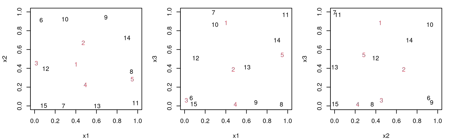
FIGURE 4.14: Augmenting design (red, numbered 1 to 5) in three inputs via three 2d projections.

As before, any particular projection might not be perfect, but the ensemble of panel views indicates that new runs are indeed spaced out relative to themselves and to the previous locations (numbered 6:15 and colored in black). Sometimes the illusion of perspective offered by the scatterplot3d library is helpful in such inspections. Some code is provided below, but graphical output is suppressed due to the excessive whitespace it creates in the Rmarkdown environment.

library(scatterplot3d)
scatterplot3d(X, type="h", color=c(rep(2,5), rep(1,10)), 
  pch=c(rep(20,5), rep(21,10)), xlab="x1", ylab="x2", zlab="x3")

The color and point scheme indicates new locations $X_{n'}$ as red filled circles and $X^{\mathrm{orig}}_{n}$ as black open circles. Vertical lines under the dots, as provided by type="h", are essential to visually track locations in 3d space and see that the design is truly space-filling. Unfortunately, it’s not obvious how to use text to plot indices rather than points in scatterplot3d.

4.3 Libraries and hybrids

Our mylhs function from §4.1, and its extension mylhs.beta (§4.1.2) are hard to improve upon in terms of computational efficiency. Nevertheless it’s simpler to rely on canned alternatives. Similar functionality is offered by randomLHS in the lhs library (Carnell 2018) on CRAN. Although tailored to uniform marginals, that library does offer a sequential alternative in augmentLHS.

The lhs package also provides a nice hybrid between maximin and LHS in maximinLHS which helps avoid aliasing problems of both ordinary LHS and maximin designs. Think of this as entertaining candidate LHSs and preferring ones whose minimum distance between design element pairs is large (MD Morris and Mitchell 1995). Typical search methods proceed similarly to our sequential maximin method, described above, usually involving stochastic exchange of pairs of levels, separately (and possibly also randomly) in each coordinate, in order to preserve a Latin square structure. To compare/contrast with some of our earlier examples, code below builds one of these hybrid designs.

library(lhs)
X <- maximinLHS(10, 2)

As shown in Figure 4.15, the resulting points are spread out, but perhaps not as spread out as a fully maximin design. By default, maximinLHS performs a greedy, stepwise search. A homework exercise (§4.4) demonstrates that it’s possible to get better maximin LHS hybrid performance with a more exhaustive search. The library doesn’t provide a Latin square grid on output, so code supporting Figure 4.15 offers an educated guess as to what that grid might look like.

plot(X, xlim=c(0,1), ylim=c(0,1), xlab="x1", ylab="x2")
abline(h=seq(0,1,length=11), col="gray", lty=2)
abline(v=seq(0,1,length=11), col="gray", lty=2)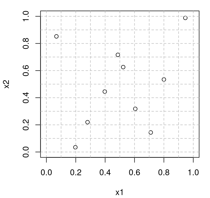

FIGURE 4.15: Maximin/LHS hybrid design.

Since it’s still an LHS, points are not pushed to the boundaries. One-dimensional uniformity guarantees at most one point near each edge. Consequently such designs are often more desirable than an LHS or maximin on their own, although there are reasons to prefer these original, raw (un-hybridized), options. For example, I’m not aware of any software offering a sequential update to a hybrid maximin LHS design. Related, so-called maximum projection design (Joseph, Gul, and Ba 2015), extends the LHS one-dimensional uniformity property to larger subspaces. Building a maxpro design entails calculations similar to those involved in maximin, and like maximin they emit a natural sequential analog. A package is available on CRAN called MaxPro (Ba and Joseph 2018). Sometimes computer experiments contain factor-valued inputs – i.e., categorical rather than real-valued ones. Maxpro designs have recently been extended to accommodate this case. Maximin “sliced” LHD (SLHD) hybrids (Ba, Myers, and Brenneman 2015) also represent an attractive option in this setting. See SLHD (Ba 2015) on CRAN.

A package called maximin (Sun and Gramacy 2019) on CRAN offers batch and sequential (ordinary) maximin design. By optionally including distance to boundaries in search criteria it can avoid sites selected along extremities of the input space. Its implementation addresses many of the computational inefficiencies highlighted for mymaximin in §4.2.1, and which are the subject of an exercise in §4.4. Additionally maximin replaces random search with a heuristically motivated derivative-based optimization, leveraging local continuity in the objective criteria. Sometimes, however, a more discrete alternative is handy. A function maximin.cand allows search to be restricted to a candidate grid, which can be helpful when simulators only accept certain input locations. A homework exercise in §5.5 requires such a feature in order to work with surrogate LGBB data from §2.1. Sun, Gramacy, Haaland, Lu, et al. (2019) used candidate-restricted sequential maximin designs to combine field and simulation data for a solar irradiance forecasting project. Obtaining accurate IBM PAIRS simulations of solar irradiance, emphasizing ones geographically far from sporadically spaced weather station data, required limiting future simulation runs to a particular grid.

There are many further options when it comes to sensible, and computationally efficient, model-free space-filling designs. DiceDesign on CRAN (Franco et al. 2018; Dupuy, Helbert, and Franco 2015) covers several others in addition ones I’ve introduced/pointed to above. We now have everything we need to move on to GP modeling in Chapter 5, in particular to generate data for illustrative examples provided therein. As mentioned at the outset of this chapter, topics in model-based design (using GPs) in Chapter 6 are in many ways twinned with the model-free analogs here. Despite conditioning on the model, resulting designs are quite similar to more agnostic alternatives, except when you have something more particular in mind. Perhaps that explains the popularity of a model-free option: all of the effect of “knowing” the model for the purposes of learning more about it, without potential for pathology as inherent in any presumptive choice before learning actually takes place.

Unfortunately, that characterization is not quite right because choosing a space-filling design can indeed influence what you learn. In fact B. Zhang, Cole, and Gramacy (2020) very specifically demonstrate pathological behavior when using space-filling designs like maximin and LHS with GP surrogates. Poor behavior can be particularly acute when using maximin or LHS as a small seed design in order to initiate an inherently sequential analysis, such as in Bayesian optimization (Chapter 7). Surprisingly, simple completely random design can protect against such pathologies. Going further, Zhang et al. show how designs offering more control on the distribution of pairwise distances – as opposed to attempting to maximize the smallest of those – fare better too. The reason has to do with mechanisms behind how GPs are typically specified, and fit to data. But we’re getting well ahead of ourselves. I must first introduce the GP.

4.4 Homework exercises

These exercises give the reader an opportunity to explore space-filling design properties and algorithms. Throughout, use up to T=10000 iterations for your searches.

#1: Faster maximin

This question targets improvements to our initial, inefficient mymaximin implementation in §4.2.1. In each case, measure improvement in terms of the rate of increase in minimum distance over search iterations.

Fix a random design Xinit of size n=100 in m=2 dimensions. Modify mymaximin to use Xinit as its starting design, and to keep track (and return) md progress over the T iterations of search. (It might help to change the default number of iterations to T=10000.) Generate a maximin design using your new mymaximin implementation. Provide a visual of the final design and progress in md over the iterations. Report execution time.
Update mymaximin to more cleverly choose the row swapped out in each iteration. Argue that only two rows are worth potentially swapping out if progress is to be measured by increasing md over stochastic exchange iterations. How would you choose among these two? After you implement your new scheme, compare it to results from #a via visuals of the final design and md progress on common axes. Compare the execution time to #a.
Update mymaximin so that not all pairwise distances are calculated in each iteration. Calculate and update only those distances, and minimum pairwise distances, which change. Verify that your new implementation gives identical results (final design and md progress) to those which you obtained in #b, but show that the calculation is now much faster in terms of execution time. If your algorithm is randomized, verifying identical results will require identical RNG seeds.
Repeat #a–c thirty times with novel Xinit and compare average progress in md in terms of means and 90% quantiles for each of the three methods. Also compare distributions of compute times.

#2: Hybrid space-filling design

Latin hypercube samples (LHSs) (§4.1) and maximin distance (§4.2) are both space-filling in a certain sense. Consider a hybrid of the two methods, a so-called maximin LHS (§4.3) as introduced by MD Morris and Mitchell (1995). That is, among LHSs we desire ones that maximize the minimum distance between design points. Such a hybrid can offer the best of both worlds: nice margins (whether uniform or otherwise), no clumping at the boundaries, and no diagonal aliasing!

There are lots of ways to make a precise definition for maximin LHS, but the spirit is conveyed in a simple algorithm for how it might be (approximately) calculated.

Generate an initializing LHS Xinit of appropriate size.
Randomly choose a pair of design points, randomly choose a column, and propose swapping that pair’s coordinates in that column.
Keep the exchange if the minimum distances between those two points and all others is improved; otherwise swap back.
Repeat 2–3.

Your task is the following.

Convince yourself (and your instructor) that the result is still an LHS.
Implement the method and try it out in $m \in \{2, 3, 4\}$ dimensional design spaces, with design sizes $n \in \{100, 1000\}$. How do your maximin LHS designs compare to maximin? In particular, how do 2d projections for $m \in \{3,4\}$ compare? Can you improve upon the numerical performance of your algorithm by deploying some of the strategies from exercises #1b–c?
Report on average progress of the algorithm, in terms of its ability to maximize minimum distance(s), over iterations of steps 2–3 above. (Use Monte Carlo; e.g., see #1d above.)
How does your algorithm compare to the maximinLHS method in the lhs library for R?

(The attentive reader will recognize that the choice of random jitter in the Latin square, i.e., the U step in generating Xinit, is at odds with the maximin criterion. But let’s not get distracted by such details here; if you prefer choose U=0.)

#3: $\phi_p$ designs

In addition to maximin LHS hybridization (#2 above), MD Morris and Mitchell (1995) suggested the following search criteria for the purpose of space-filling design. Let $d_k$, for $k=1,\dots,K$, denote the $K$ unique pairwise distances in a design $X_n$, and let $J_k$ denote the number of rows of $X_n$ who share pairwise distance $d_k$. In most applications, $K = {n \choose 2}$ and all $J_k = 1$. Then, one may search for a design $X_n$ by minimizing $\phi_p(X_n)$ where

\[ \phi_p = \left[ \sum_{k=1}^K J_k d_k^{-p} \right]^{1/p}. \]

At $p = \infty$, minimizing the criterion is equivalent to solving for a maximin design. Interestingly, Morris & Mitchell show how all $p$ lead to maximin designs – in the sense that the smallest distance, $\min_k d_k$ is maximized – but resulting designs differ in the distribution of other distances $d_{(-k)}$. Behavior of numerical methods for optimizing $\phi_p$ also differ from maximin due to the smoother nature of the criteria for smaller $p$.

Your task is to port mymaximin to myminphi, entertain enhancements similar to those of exercises #1a–c (i.e., think about search and computational efficiency), and to make a Monte Carlo comparison to those methods by extending #1d. Limit your study to $p \in \{2,5\}$. Then hybridize with LHS following exercise #2b–c. How do the most efficient variations on the four methods: maximin, $\phi_p$, maximin LHS, and $\phi_p$ LHS compare?

#4: Candidate-based augmenting maximin design

For a solar irradiance forecasting project, Sun, Gramacy, Haaland, Lu, et al. (2019) worked with data from a network of weather stations scattered throughout the continental United States. Monitoring sites are heterogeneously dispersed, with heavy concentration in national/state parks and sparse coverage in the Great Plains and lower Midwest. Code below reads in the data …

lola <- read.csv("lola.csv")

… and Figure 4.16 offers a visual of the sites where irradiance measurements have been gathered.

library(maps)
myUS <- map("state", fill=TRUE, plot=FALSE)
omit <- c("massachusetts:martha's vineyard", "massachusetts:nantucket", 
  "new york:manhattan", "new york:staten island", "new york:long island", 
  "north carolina:knotts", "north carolina:spit", "virginia:chesapeake", 
  "virginia:chincoteague", "washington:san juan island", 
  "washington:lopez island", "washington:orcas island", 
  "washington:whidbey island")
myNames <- myUS$names[!(myUS$names %in% omit)]
myUS <- map("state", myNames, fill=TRUE, col="gray", plot=TRUE)
points(lola$lon, lola$lat, pch=19, cex=0.3, col="blue")
legend("bottomleft", legend=c("Original/Weather Stations"), col="blue", 
  pch=19, pt.cex=0.3, bty="n")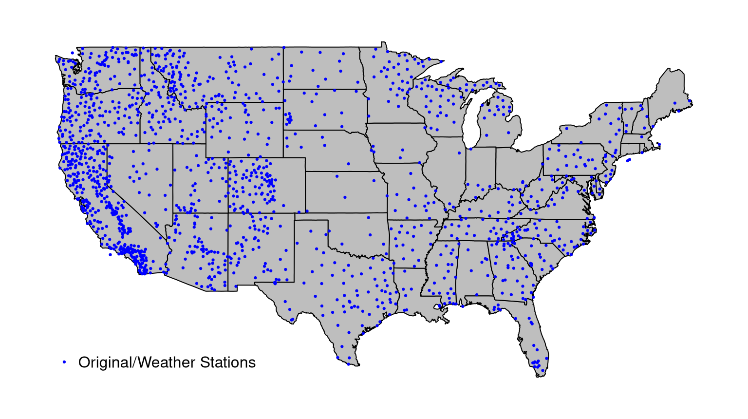

FIGURE 4.16: Weather station sites in the continental USA.

To extrapolate better to sparsely covered regions of the country, Sun, Gramacy, Haaland, Lu, et al. (2019) augmented their data with computer model irradiance evaluations. For reasons that are somewhat more thoroughly explained in §4.3 and in their manuscript, such runs could only be obtained at the grid of locations stored in the file below.

lola.cands <- read.csv("lola_cands.csv")

Demonstrate visually that the grid uniformly covers the continental USA except where it doubles-up on original lola locations. For brownie points, how would you automate the process of creating lola.cands from a uniform 0.1-spaced grid in longitude and latitude throughout myUS$range; that is, so that there are no grid points in the oceans/Great Lakes and none overlapping with lola?
Design an algorithm which delivers 100 new sites whose locations are confined to lola.cands and whose minimum distance to themselves and to lola is maximized. Augment the visualization above to include the newly selected sites. Inspect md progress over the iterations. You may wish to adapt your method from exercise #1.
Using your implementation from #b, or with maximin.cands in the maximin package on CRAN, select 900 more (for 1000 total) new sites and provide visuals of the results. Plot md progress over the iterations.

References

Ba, S. 2015. SLHD: Maximin-Distance (Sliced) Latin Hypercube Designs. https://CRAN.R-project.org/package=SLHD.

Ba, S, and VR Joseph. 2018. MaxPro: Maximum Projection Designs. https://CRAN.R-project.org/package=MaxPro.

Ba, S, WR Myers, and WA Brenneman. 2015. “Optimal Sliced Latin Hypercube Designs.” Technometrics 57 (4): 479–87.

Carnell, Rob. 2018. lhs: Latin Hypercube Samples. https://CRAN.R-project.org/package=lhs.

Dupuy, D, C Helbert, and J Franco. 2015. “DiceDesign and DiceEval: Two R Packages for Design and Analysis of Computer Experiments.” Journal of Statistical Software 65 (11): 1–38. http://www.jstatsoft.org/v65/i11/.

Franco, J, D Dupuy, O Roustant, P Kiener, G Damblin, and B Iooss. 2018. DiceDesign: Designs of Computer Experiments. https://CRAN.R-project.org/package=DiceDesign.

Gneiting, T, and AE Raftery. 2007. “Strictly Proper Scoring Rules, Prediction, and Estimation.” Journal of the American Statistical Association 102 (477): 359–78.

Gramacy, RB. 2014. plgp: Particle Learning of Gaussian Processes. https://CRAN.R-project.org/package=plgp.

Johnson, ME, LM Moore, and D Ylvisaker. 1990. “Minimax and Maximin Distance Designs.” Journal of Statistical Planning and Inference 26 (2): 131–48.

Joseph, VR, En Gul, and S Ba. 2015. “Maximum Projection Designs for Computer Experiments.” Biometrika 102 (2): 371–80.

Lin, CD, and B Tang. 2015. “Latin Hypercubes and Space-Filling Designs.” Handbook of Design and Analysis of Experiments, 593–625.

Morris, MD, and TJ Mitchell. 1995. “Exploratory Designs for Computational Experiments.” Journal of Statistical Planning and Inference 43 (3): 381–402.

Qian, PZG. 2009. “Nested Latin Hypercube Designs.” Biometrika 96 (4): 957–70.

Sun, F, and RB Gramacy. 2019. maximin: Space-Filling Design Under Maximin Distance.

Sun, F, RB Gramacy, B Haaland, S Lu, and Y Hwang. 2019. “Synthesizing Simulation and Field Data of Solar Irradiance.” Statistical Analysis and Data Mining 12 (4): 311–24.

Tan, MHY. 2013. “Minimax Designs for Finite Design Regions.” Technometrics 55 (3): 346–58.

Zhang, B, DA Cole, and RB Gramacy. 2020. “Distance-Distributed Design for Gaussian Process Surrogates.” To Appear in Technometrics.