1.3 Polar form in the Euclidean plane

In this section we will focus on vectors in $\mathbb{R}^2$, and consider a different way of representing them. As well as defining a vector in $\mathbb{R}^2$ based on its components in the $x$ and $y$ directions, we could also define it based on its length and its angle from the $x$-axis. This is known as polar form, and is illustrated in Figure 1.4.

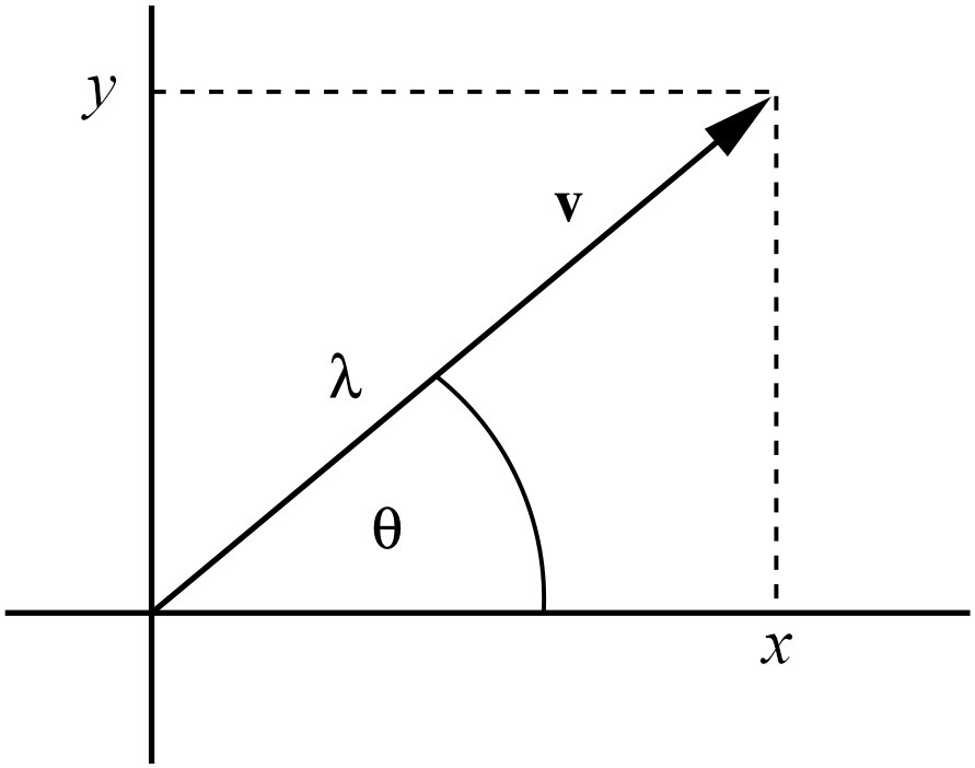
Figure 1.4: A vector $v$ in $\mathbb{R}^2$ represented by Cartesian coordinates $(x,y)$ or by polar coordinates $\lambda, \theta$. We have $x=\lambda\cos\theta$, $y=\lambda \sin\theta$, $\lambda=\sqrt{x^2+y^2}$ and $\tan\theta=\dfrac{y}{x}$.

In particular, a unit vector has length one, hence all unit vectors lie on the circle of radius one in $\mathbb{R}^2$, and a unit vector is determined solely by its angle $\theta$ with the $x$-axis. By elementary geometry we find that the unit vector with angle $\theta$ to the $x$-axis is given by $$\label{eq:unitvec} u(\theta):=\begin{pmatrix}\cos\theta\\ \sin\theta\end{pmatrix}.$$

We can then multiply by a scalar order to obtain any vector in $\mathbb{R}^2$, and this gives us a unique vector. In particular, the scalar that we multiply our unit vector by is the norm of the vector.

Theorem 1.18:

For every $v\in\mathbb{R}^2$, $v\neq 0$, there exist unique $\theta\in [0,2\pi)$ and $\lambda\in (0,\infty)$ with $$v=\lambda u(\theta)$$

Proof.

Given $v=\begin{pmatrix}v_1\\ v_2\end{pmatrix}\neq 0$ we have to find $\lambda>0$ and $\theta\in [0,2\pi)$ such that $$\begin{pmatrix}v_1\\ v_2\end{pmatrix}=\lambda u(\theta)=\begin{pmatrix}\lambda \cos \theta\\ \lambda \sin\theta\end{pmatrix}.$$ Since $\lVert\lambda u(\theta)\rVert=\lambda\lVert u(\theta)\rVert=\lambda$ (note that $\lambda>0$, hence $\lvert\lambda\rvert=\lambda$) we get immediately $$\lambda=\lVert v\rVert.$$ To determine $\theta$ we have to solve the two equations $$\cos\theta=\frac{v_1}{\lVert v\rVert} ,\quad \sin\theta=\frac{v_2}{\lVert v\rVert} ,$$ which is in principle easy, but we have to be a bit careful with the signs of $v_1,v_2$. If $v_2>0$ we can divide the first by the second equation and obtain $\cos\theta/\sin\theta=v_1/v_2$, hence $\theta=\cot^{-1} \frac{v_1}{v_2},$ that is $$\theta=\arctan\frac{v_2}{v_1}\in (0,\pi) .$$ If $v_1>0$ and $v_2 < 0$ we have $\arctan (v_2/v_1) \in (-\frac{\pi}{2},0)$ and so $\theta=2\pi+\arctan (v_2/v_1)$; analogous arguments apply in the remaining cases and this is illustrated in Figure 1.5.

□

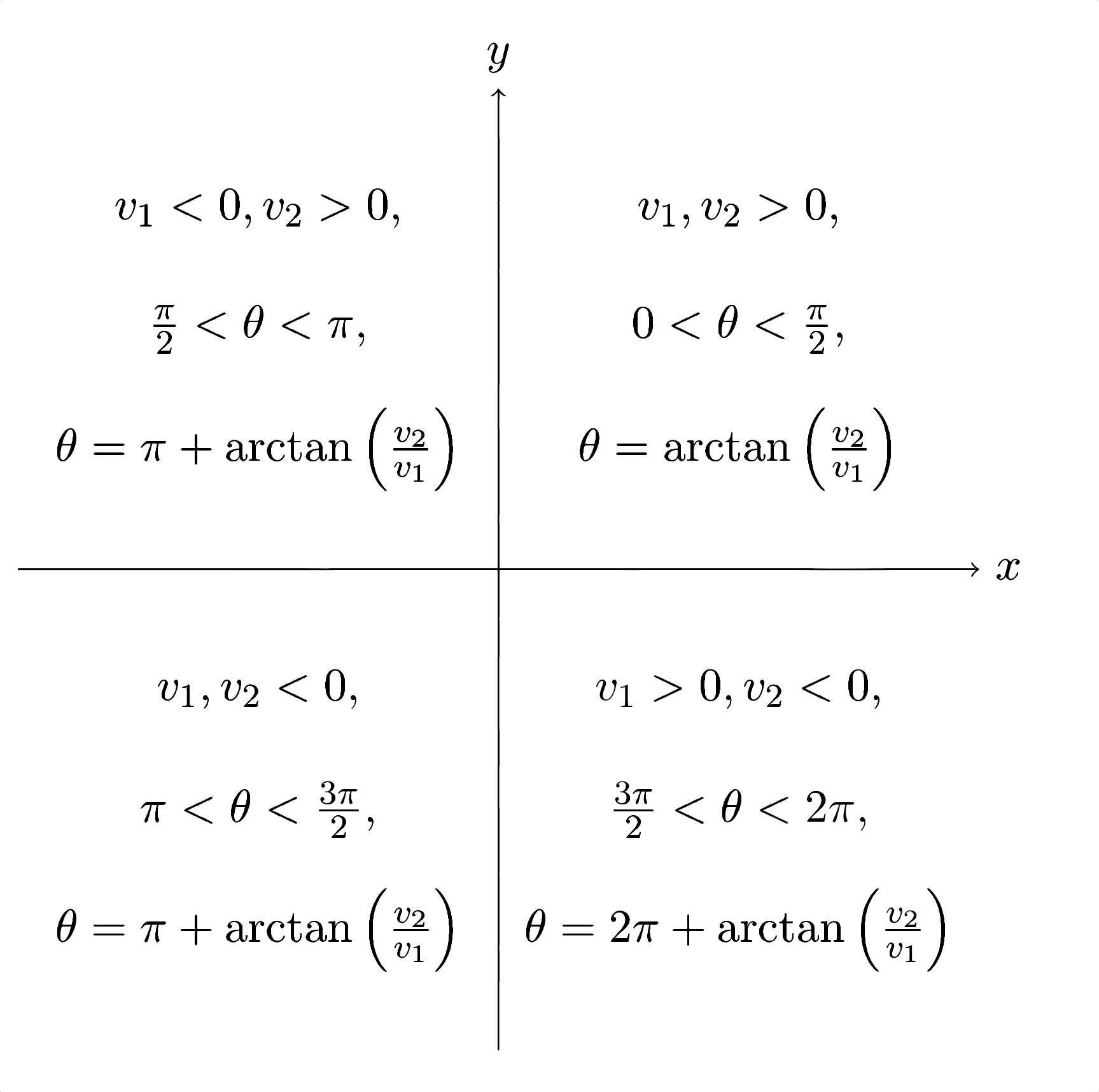
Figure 1.5: How to calculate the argument for $(v_1,v_2)$ in each quadrant of the Euclidean plane.

The converse of this result also holds, that is given $\theta\in [0,2\pi)$ and $\lambda\geq 0$ we get a unique vector with direction $\theta$ and length $\lambda$: $$v=\lambda u(\theta)=\begin{pmatrix}\lambda\cos\theta\\ \lambda\sin\theta\end{pmatrix}.$$

Exercise 1.19:

Let $v=\begin{pmatrix} -1 \\ \sqrt{3}\end{pmatrix}$. Find $\lambda\in (0, \infty]$ and $\theta \in [0,2\pi)$ such that $v=\lambda u(\theta)$.

There are many practical situations where the polar form of a vector might be more useful than the Cartesian form, for example a ship navigating from a port may travel a certain distance at a given angle. In the next chapter, we will look at an extended example of vectors in $\mathbb{R}^2$, namely the complex plane, see how complex numbers can be viewed as vectors and how their polar form provides a useful insight into the geometric interpretation of multiplication.