3.1 Linear equations

The simplest linear equation is an equation of the form \[ax=b,\] where \(x\) is an unknown number which we want to determine and \(a\) and \(b\) are known real numbers with \(a\neq 0\), for example \(2x=7\). For this example we find the solution \(x=7/2\). Linear means that no powers or more complicated expressions of \(x\) occur, for instance the equations \[3 x^5-2x=3 \quad \text{and} \quad x+\cos(x)=1\] are nonlinear.

But more interesting than the case of one unknown are equations where we have more than one unknown. Let us look at a couple of simple examples.

Example 3.1:

Consider \[3x-4y=3,\] where \(x\) and \(y\) are two unknown real numbers. In this case the equation is satisfied for all \(x,y\) such that \[y=\frac{3}{4}x-\frac{3}{4} ,\] so instead of determining a single solution the equation defines a set of \(x,y\) which satisfy the equation. This set is a line in \(\mathbb{R}^2\).

Example 3.2:

We could add another equation and consider the solutions to two equations, for example \[3x-4y=3 \quad \text{and}\quad 3x+y=1.\] In this example we again find a single solution. Subtracting the second equation from the first gives \(-5y=2\), hence \(y=-2/5\) and then from the first equation \(x=1+\frac{4}{3}y=7/15\). Another way to look at the two equations is that they define two lines in \(\mathbb{R}^2\) and the joint solution is the intersection of these two straight lines, as depicted in Figure 3.1.

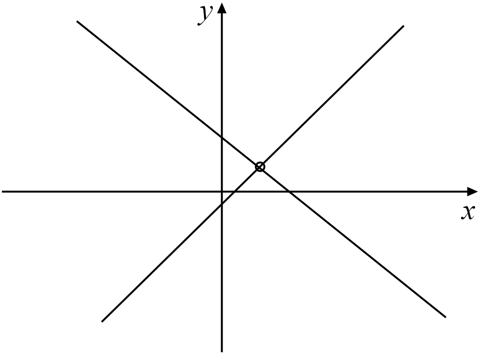
Figure 3.1: A system of two linear equations in two unknowns \((x,y)\) which determines two lines; their intersection gives the solution.

Example 3.3:

If we look instead at the slightly modified system of two equations \[3x-4y=3 \quad \text{and} \quad -6x+8y=0 ,\] then we find that these two equations have no solutions. To see this we multiply the first equation by \(-2\), and then the set of two equations becomes \[-6x+8y=6\quad \text{and},\quad -6x+8y=0 ,\] so the two equations contradict each other and the system has no solutions. Geometrically speaking this means that the straight lines defined by the two equations have no intersection, that is they are parallel, as depicted in Figure 3.2.

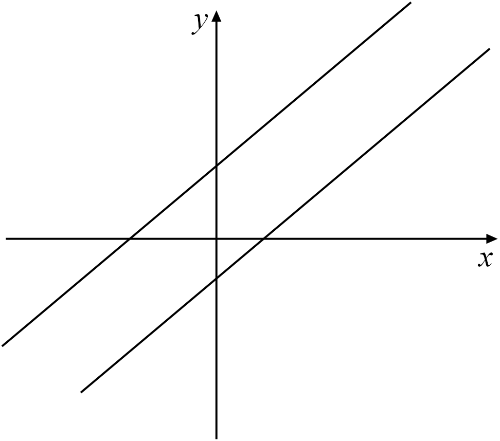
Figure 3.2: A system of two linear equations in two unknowns \((x,y)\) where the corresponding lines have no intersection, hence the system has no solution.

So above we have found examples of systems of linear equations which have exactly one solution, many solutions, and no solutions at all. We will see in the following that these are all the possible outcomes which can occur in general. So far we have talked about linear equations but haven’t really defined them in general, so we now do so below.

Definition 3.4: (Linear equation)

A linear equation in \(n\) variables \(x_1,x_2,\cdots ,x_n\) is an equation of the form \[a_1 x_1+a_2x_2+\cdots +a_nx_n=b\] where \(a_1,a_2,\cdots ,a_n\) and \(b\) are given numbers. These are known as the coefficients of the equation.

In the rest of this chapter, the numbers \(a_1,a_2,\cdots ,a_n\) and \(b\) will be real numbers, and the solutions we are searching for will also be real numbers; however there may be other settings where the coefficients and/or solutions are taken from different sets. For example we could allow our coefficents and solutions to be complex numbers rather than real numbers, and then by replacing every instance of \(\mathbb{R}\) with \(\mathbb{C}\) the corresponding results would follow in the same way.

In this course we will often be interested in systems of linear equations.

Definition 3.5: (System of linear equations)

A system of \(m\) linear equations in \(n\) unknowns \(x_1,x_2,\cdots ,x_n\) is a collection of \(m\) linear equations of the form \[\begin{aligned} a_{11}x_1+a_{12}x_2+\cdots +a_{1n}x_n&= b_1\\ a_{21}x_1+a_{22}x_2+\cdots +a_{2n}x_n&= b_2\\ \vdots\qquad\vdots\qquad &= \vdots\\ a_{m1}x_1+a_{m2}x_2+\cdots +a_{mn}x_n&= b_m \end{aligned}\] where the coefficients \(a_{ij}\) and \(b_j\) are given numbers.

When we ask for a solution \(x_1,x_2,\cdots, x_n\) to a system of linear equations, then we ask for a set of numbers \(x_1,x_2,\cdots ,x_n\) which satisfy all \(m\) equations simultaneously.

One often looks at the set of coefficients \(a_{ij}\) defining a system of linear equations as an independent entity in its own right.

Definition 3.6: (Matrix)

For \(m,n\in \mathbb{N}\), a \(m\times n\) matrix \(A\) (an “\(m\) by \(n\)” matrix) is a rectangular array of numbers \(a_{ij}\in \mathbb{R}\), \(i=1,2,\ldots,m\) and \(j=1,\ldots, n\) of the form \[\label{mf} A=\begin{pmatrix}a_{11} & a_{12} & \cdots & a_{1n} \\ a_{21} & a_{22} & \cdots & a_{2n} \\ \vdots & \vdots & \ddots &\vdots \\ a_{m1} & a_{m2} & \cdots & a_{mn} \end{pmatrix}\] The numbers \(a_{ij}\) are called the elements of the matrix \(A\), and we often write \(A=(a_{ij})\) to denote the matrix \(A\) with elements \(a_{ij}\). The set of all \(m\times n\) matrices with real elements will be denoted by \[M_{m,n}(\mathbb{R}) ,\] and if \(n=m\) we will write \[M_n(\mathbb{R}) .\]

One can similarly define matrices with elements in other sets, e.g,. \(M_{m,n}(\mathbb{C})\) is the set of matrices with complex elements.

Note: The plural of matrix is matrices.

Example 3.7:

An example of a \(3\times 2\) matrix is \[\begin{pmatrix}1 & 3\\ -1& 0 \\ 2& 2\end{pmatrix}.\]

An \(m\times n\) matrix has \(m\) rows and \(n\) columns. The \(i\)th row of \(A=(a_{ij})\) is \[\begin{pmatrix} a_{i1} & a_{i2} & \cdots & a_{in} \end{pmatrix}\] and is naturally identified as a row vector \((a_{i1},a_{i2}, \cdots, a_{in})\in\mathbb{R}^n\) with \(n\) components. The \(j\)th column of \(A\) is \[\begin{pmatrix} {a_{1j}} \\ {a_{2j}} \\ {\vdots} \\ {a_{mj}} \end{pmatrix} ,\] which is a column vector in \(\mathbb{R}^m\) with \(m\) components.

Example 3.8:

For the matrix in Example 3.7 the first and second column vectors are \[\begin{pmatrix}1\\ -1\\2\end{pmatrix}\text{and}\quad \begin{pmatrix}3\\0\\2\end{pmatrix},\] respectively, and the first, second and third row vectors are \[\begin{pmatrix}1 & 3\end{pmatrix}, \quad \begin{pmatrix}-1 & 0\end{pmatrix}, \quad \text{and} \quad \begin{pmatrix}2 & 2\end{pmatrix}.\]

There is one somewhat unpleasant notational subtlety here. Take, say a vector \((3,4)\in \mathbb{R}^2\). This vector can be written as a matrix either as a \(1\times 2\) matrix \(( 3 \;4)\), with just one row or a \(2\times 1\) matrix \(\begin{pmatrix}3\\ 4\end{pmatrix}\), with just one column. To avoid confusion, we need a convention whether we are going to identify vectors with row or column matrices, which will later lead us to the general concept of the transpose of a matrix.

The standard convention is to identify a vector \(x=(x_1,\ldots,x_n)\in \mathbb{R}^n\) with a column-matrix (or column-vector) \[x=(x_1,\ldots,x_n) =\begin{pmatrix}x_1 \\ \vdots \\ x_n\end{pmatrix},\] but bear in mind that the same quantity can also be represented by a row-matrix (or row-vector) \[x^t = (x_1\;\ldots\;x_n).\] To distinguish, with the boldface notation, between row and column-matrices, representing a single vector, we will use the superscript \({}^t\) (to be read “transpose”, this will be discussed further later in the chapter) for row-matrices. The difference between the latter two formulae is that we do not use comas to separate elements of row-matrices.

When dealing with matrices it will often be useful to write them in terms of their rows or in terms of their columns. That is, if the rows of \(A\) are \(r_1^t, r_2^t, \ldots, r_m^t\) (for now, think of the superscript \(t\) as notation so that we remember they are rows) we may write \[A = \begin{pmatrix} \cdots & r_1^t & \cdots \\ \cdots & r_2^t & \cdots \\ & \vdots & \\ \cdots & r_m^t & \cdots \end{pmatrix} \text{ or just } A = \begin{pmatrix} r_1^t \\ r_2^t \\ \vdots \\ r_m^t \end{pmatrix},\] and if the columns of \(A\) are \(c_1, \ldots, c_n\) then we may write \[A = \begin{pmatrix} \vdots & \vdots & & \vdots \\ c_1 & c_2 & \cdots & c_n \\ \vdots & \vdots && \vdots \end{pmatrix} \text{ or just } A = \begin{pmatrix} c_1 & c_2 & \cdots & c_n \end{pmatrix}.\]

In Definition 3.5, the rows of the matrix of coefficients are combined with the \(n\) unknowns to produce \(m\) numbers \(b_i\), we will take these formulas and turn them into a definition for the action of \(m\times n\) matrices on vectors with \(n\) components:

Definition 3.9:

Let \(A=(a_{ij})\) be an \(m\times n\) matrix and \(x\in \mathbb{R}^n\) with components \(x=(x_1, x_2,\cdots, x_n)\), then the action of \(A\) on \(x\) is defined by \[\label{ax} Ax:=\begin{pmatrix}a_{11} x_1 + a_{12} x_2+\cdots +a_{1n} x_n \\ a_{21} x_1 + a_{22} x_2+\cdots +a_{2n} x_n\\ \vdots \\ a_{m1} x_1 + a_{m2} x_2+\cdots +a_{mn} x_n\end{pmatrix}%= \bpm \ba^t_1\cdot\bx \\ \ba_2^t \cdot \bx \\ \vdots \\ \ba^t_m \cdot\bx \epm \in \mathbb{R}^m.\]

Note that \(Ax\) is a vector in \(\mathbb{R}^m\) and if we write \(y=Ax\) then the components of \(y\) are given by \[\begin{equation}y_i=\sum_{j=1}^n a_{ijx_j} \tag{3.1}\end{equation}\] which is the dot-product between \(x\) and the \(i\)th row vector of \(A\). The action of \(A\) on elements of \(\mathbb{R}^n\) is a map from \(\mathbb{R}^n\) to \(\mathbb{R}^m\), i.e., \[A:\mathbb{R}^n\to\mathbb{R}^m .\]

Using the notation of matrices and their action on vectors, a system of linear equations of the form in Definition 3.5 can now be rewritten as \[\begin{equation}Ax=b. \tag{3.2}\end{equation}\] So using matrices allows us to write a system of linear equations in a much more compact way.

Another way of looking at the action of a matrix on a vector is as follows: Let \(a_1, a_2, \cdots, a_n\in\mathbb{R}^m\) be the column vectors of \(A\), then \[\begin{equation} Ax=x_1a_1+x_2a_2+\cdots +x_na_n. \tag{3.3}\end{equation}\] So \(Ax\) is a linear combination of the column vectors of \(A\) with coefficients given by the components of \(x\). This relation follows directly from (3.1). Solving \(Ax=b\) means that we want to find coefficients \((x_1,\ldots,x_n)\) so that \(b\) may written as a linear combination of the column-vectors of the matrix \(A\). Such a linear combination may or may not exist, and if it exists may or may not be unique.

Exercise 3.10:

Which matrix equation is equivalent to the system \(3x+5y-z=0, y-2x=5, x+5y+2z=9\)?

The map \(A:\mathbb{R}^n \to \mathbb{R}^m\) has the important property that it respects addition (meaning that we can add two vectors and then apply the map or apply the map separately and then add the results and get the same outcome) and scalar multiplication (similarly), as demonstrated in the following theorem.

Theorem 3.11:

Let \(A\) be an \(m\times n\) matrix, then the map defined in Definition 3.9 satisfies the two properties

• \(A(x+y)=Ax+Ay\) for all \(x,y\in \mathbb{R}^n\),

• \(A(\lambda x)=\lambda Ax\) for all \(x\in\mathbb{R}^n\) and \(\lambda\in\mathbb{R}\).

Proof.

This is most easily shown using (3.1). Let us denote the components of the vector \(A(x+y)\) by \(z_i\), \(i=1,2,\cdots, m\), i.e., \(z=A(x+y)\) with \(z=(z_1,z_2,\cdots, z_m)\). Then by (3.1) \[z_i=\sum_{j=1}^n a_{ij}(x_j+y_j)=\sum_{j=1}^n a_{ij}x_j+\sum_{j=1}^na_{ij}y_j ,\] and on the right hand side we have the sum of the \(i\)th components of \(Ax\) and \(Ay\), again by (3.1). The second assertion \(A(\lambda x)=\lambda Ax\) follows again directly from (3.1) and is left as a simple exercise.

□

Before we start solving systems of linear equations let us study matrices in some more detail.