6.2 Bases and dimension

In Section 5.2 we explored how we can build a space from a set of vectors by taking their span, and the concept of linear independence now gives us a way to prevent any redundancy in our choice of vectors in the spanning set.

So if a collection of vectors span a subspace and are linearly independent, then they deserve a special name.

Definition 6.15:

Let \(V\subseteq W\) be a linear subspace of a vector space \(W\). A basis of \(V\) is a set of vectors \(v_1,v_2 \cdots ,v_k\in V\) such that

• \(\operatorname{span}\{v_1,v_2 \cdots ,v_k\}= V\), and

• the vectors \(v_1,v_2 \cdots ,v_k\in V\) are linearly independent.

The plural of basis is bases.

So a basis of \(V\) is a set of vectors in \(V\) which generate the whole subspace \(V\), but with the minimal number of vectors necessary.

Example 6.16:

The set \(e_1=(1,0,0, \cdots ,0)\), \(e_2=(0,1,0,\cdots ,0)\), \(e_3=(0,0,1,\cdots ,0)\), ... , \(e_n=(0,0,0, \cdots ,1) \in \mathbb{R}^n\) is a basis for \(\mathbb{R}^n\) over \(\mathbb{R}\). For any \(v\in \mathbb{R}^n\) we have \[v=(x_1,x_2, \cdots ,x_n)=x_1e_1+x_2e_2+\cdots +x_ne_n,\] so this is a spanning set for \(\mathbb{R}^n\) and is linearly independent since the corresponding matrix is \(I\in M_n(\mathbb{R}).\)

Definition 6.17: (Standard basis)

The set \(e_1=(1,0,0, \cdots ,0)\), \(e_2=(0,1,0,\cdots ,0)\), \(e_3=(0,0,1,\cdots ,0)\), ... , \(e_n=(0,0,0, \cdots ,1) \in \mathbb{R}^n\)is called the standard basis for \(\mathbb{R}^n\) over \(\mathbb{R}\).

Exercise 6.18:

Is \(e_1, \dots, e_n \in \mathbb{C}^n\) a basis for \(\mathbb{C}^n\) over \(\mathbb{C}\)? What about over \(\mathbb{R}\)?

Click for solution

Yes, this is a basis for \(\mathbb{C}^n\) over \(\mathbb{C}\) by a similar argument to the example above (and we may similarly refer to this as the standard basis for \(\mathbb{C}^n\) over \(\mathbb{C}\)). However it is not a basis for \(\mathbb{C}^n\) over \(\mathbb{R}\) as it is not a spanning set, since there is no \(\mathbb{R}\)-linear combination of these vectors that give \((i, 0, \dots, 0)\) for example.

An example of a basis for \(\mathbb{C}^n\) over \(\mathbb{R}\) would be \(e_1, \dots, e_n, ie_1, \dots, ie_n\).

 

The definition a basis means that every vector can be written as a linear combination of basis vectors in a unique way.

Theorem 6.19:

Let \(W\) be a vector space over \(\mathbb{F}\), \(V\subseteq W\) be a linear subspace, and \(v_1,v_2 \cdots ,v_k\in V\) a basis of \(V\). Then for any \(v\in V\) there exist a unique set of scalars \(\lambda_1,\lambda_2, \cdots ,\lambda_k\in\mathbb{F}\) such that \[v=\lambda_1v_1+\lambda_2v_2+\cdots+\lambda_kv_k .\]

Proof.

Since the vectors \(v_1,v_2 \cdots ,v_k\) span \(V\) there exist for any \(v\in V\) scalars \(\lambda_1,\lambda_2, \cdots ,\lambda_k\in\mathbb{F}\) such that \[\begin{equation} v=\lambda_1v_1+\lambda_2v_2+\cdots+\lambda_kv_k. \tag{6.2}\end{equation}\] We have to show that these scalars are unique. So let us assume there is another, possibly different, set of scalars \(\mu_1,\mu_2,\cdots ,\mu_k\) with \[\begin{equation} v=\mu_1v_1+\mu_2v_2+\cdots +\mu_kv_k, \tag{6.3}\end{equation}\] then subtracting (6.2) from (6.3) gives \[0=(\mu_1-\lambda_1)v_1+(\mu_2-\lambda_2)v_2+\cdots +(\mu_k-\lambda_k)v_k\] but since we assumed that the vectors \(v_1,v_2,\cdots,v_k\) are linearly independent we get that \(\mu_1-\lambda_1=\mu_2-\lambda_2=\cdots =\mu_k-\lambda_k=0\) and hence \[\mu_1=\lambda_1 ,\quad \mu_2=\lambda_2 ,\ldots, \quad \mu_k=\lambda_k.\]

□

Bases are not unique, that is our vector spaces will have more than one choice of basis. The standard basis defined in 6.17 is a useful basis as it is very straightforward to see how we can write any given vector in terms of this basis. However, there are often good reasons for choosing different bases as well. We will see more about this later in the course, but for now we will look at some further examples of bases and some useful properties.

Example 6.20:

Consider \(v_1=(1,1)\) and \(v_2=(-1,1)\), and let us see if they form a basis of \(\mathbb{R}^2\). To check if they span \(\mathbb{R}^2\), we take an arbitrary \((x_1,x_2)\in \mathbb{R}^2\) and have to find \(\lambda_1, \lambda_2\in\mathbb{R}\) such that \[\begin{pmatrix}x_1\\ x_2\end{pmatrix}=\lambda_1v_1+\lambda_2v_2=\begin{pmatrix}\lambda_1-\lambda_2\\ \lambda_1+\lambda_2\end{pmatrix}.\] This is just a system of two linear equations for \(\lambda_1, \lambda_2\) and can be easily solved to give \[\lambda_1=\frac{x_1+x_2}{2} ,\quad \lambda_2 =\frac{-x_1+x_2}{2} ,\] hence the two vectors span \(\mathbb{R}^2\) . Furthermore if we set \(x_1=x_2=0\) we see that the only solution to \(\lambda_1v_1+\lambda_2v_2=\mathbf{0}\) is \(\lambda_1=\lambda_2=0\), so the vectors are also linearly independent, and hence we do have a basis for \(\mathbb{R}^2\).

Theorem 6.19 tells us that we can write any vector in a unique way as a linear combination of the vectors in a basis, so we can interpret the basis vectors as giving us a coordinate system, and the coefficients \(\lambda_i\) in an expansion \(v=\sum_{i}\lambda_iv_i\) are the coordinates of \(v\). See Figure 6.1 for an illustration of this idea.

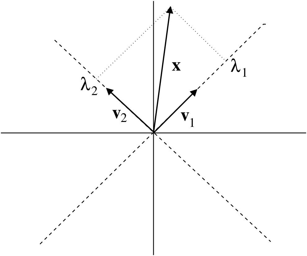
Figure 6.1: Illustrating how a basis \(v_1,v_2\) of \(\mathbb{R}^2\) acts as a coordinate system: the dashed lines are the new coordinate axes spanned by \(v_1,v_2\), and \(\lambda_1, \lambda_2\) are the coordinates of \(v=\lambda_1 v_1+\lambda_2 v_2\).

Notice that in the standard basis \(e_1, \cdots , e_n\) of \(\mathbb{R}^n\) the expansion coefficients of \(v\) are \(x_1, \cdots , x_n\), the usual Cartesian coordinates.

Exercise 6.21:

Is \(B=\{e_1, e_2, e_3\}\) a basis for \(V=\{(x, 2x,z):x,z \in \mathbb{R}\}\subseteq \mathbb{R}^3\)?

Given a basis \(v_1,v_2 \cdots ,v_k\) of \(V\) it is not always straightforward to compute the expansion of a vector \(v\) in that basis, i.e., to find the numbers \(\lambda_1,\lambda_2, \cdots ,\lambda_k\in\mathbb{F}\). In general this leads to a system of linear equations for the \(\lambda_1,\lambda_2,\cdots ,\lambda_k\).

Example 6.22:

Let us consider the set of vectors \(v_1=(1,2,3)\), \(v_2=(-1, 2,1)\) and \(v_3=(0,0,1) \in \mathbb{R}^n\). We know from Example 6.9 that they are linearly independent, so they form a good candidate for a basis of \(V=\mathbb{R}^3\) and we just have to show that they span \(\mathbb{R}^3\). Let \(w=(x,y,z)\in \mathbb{R}^3\), and then we have to find \(\lambda_1,\lambda_2,\lambda_3\) such that \[\lambda_1v_1+\lambda_2v_2+\lambda_3v_3=x.\] If we write out the components this gives a system of three linear equations for three unknowns \(\lambda_1,\lambda_2,\lambda_3\) and the corresponding augmented matrix is \[\begin{pmatrix}A & w\end{pmatrix}=\begin{pmatrix}1 & -1 &0 & x\\ 2 & 2&0 & y\\ 3 & 1& 1& z\end{pmatrix}\] and after a couple of elementary row operations (row 2\(-2\times\)row 1, row 3\(-3\times\)row 1, row 3\(-\)row 2, row 2\(\to\) (row 2)/4) we find the following row echelon form: \[\begin{pmatrix}1 & -1 & 0 &x\\ 0 & 1 & 0 & y/4-x/2\\ 0 & 0 & 1 & z-y-x\end{pmatrix}.\] Back-substitution then gives \[\lambda_3=z-y-x ,\quad \lambda_2=\frac{y}{4}-\frac{x}{2} \quad \lambda_1=\frac{y}{4}+\frac{x}{2} .\] This means that given an arbitrary vector \((x,y,z)\) we have shown how to find coefficients \(\lambda_1, \lambda_2, \lambda_3\) in order to write our vector in terms of \(v_1, v_2, v_3\) and so these vectors do span \(\mathbb{R}^3.\) Therefore the the vectors form a basis and the expansion of an arbitrary vector \(w=(x,y,z)\in\mathbb{R}^3\) in that basis is given by \[w=\bigg(\frac{y}{4}+\frac{x}{2}\bigg)v_1+\bigg(\frac{y}{4}-\frac{x}{2}\bigg)v_2+(z-y-x)v_3 .\]

We now want to show that any subspace of the vector spaces that we have been exploring will indeed have a basis. To do this we first introduce some terminology.

Definition 6.23: (Finite-dimensional vector space)

A vector space is called finite-dimensional if it can be spanned by a finite number of vectors.

So \(\mathbb{R}^n\) over \(\mathbb{R}\), \(\mathbb{C}^n\) over \(\mathbb{R}\) and \(\mathbb{C}^n\) over \(\mathbb{C}\) are all finite-dimensional

So we want to show any subspace of a finite-dimensional vector space must have a basis. This will be a consequence of the following result which says that any set of linearly independent vectors in a subspace \(V\) is either already a basis of \(V\), or can be extended to a basis of \(V\).

Theorem 6.24:

Let \(V\) be a linear subspace of a finite-dimensional vector space over \(\mathbb{F}\), and \(v_1, v_2,\cdots, v_r\in V\) be a set of linearly independent vectors. Then either \(v_1, \cdots, v_r\) are a basis of \(V\), or there exist a finite number of further vectors \(v_{r+1}, \cdots ,v_k\in V\) such that \(v_1, \cdots ,v_k\) is a basis of V.

Proof.

Let us set \[V_r:=\operatorname{span}\{v_1, v_2,\cdots, v_r\} ,\] which is a subspace with basis \(v_1, v_2,\cdots, v_r\) and \(V_r\subseteq V\).

Now if \(V_r=V\), then we are done. Otherwise, \(V_r\neq V\) and then there exists a vector \(v_{r+1}\neq \mathbf{0}\) with \(v_{r+1}\in V\) but \(v_{r+1}\notin V_r\). We claim that \(v_1, v_2,\cdots, v_r, v_{r+1}\) are linearly independent.

To show this assume \[\lambda_1v_1+\lambda_2v_2+\cdots +\lambda_rv_r+\lambda_{r+1}v_{r+1}=\mathbf{0},\] and then if \(\lambda_{r+1}\neq 0\) we get \[v_{r+1}=-\frac{\lambda_1}{\lambda_{r+1}}v_1-\frac{\lambda_2}{\lambda_{r+1}}v_2-\cdots -\frac{\lambda_r}{\lambda_{r+1}}v_r\in V_r\] which contradicts our assumption \(v_{r+1}\notin V_r\). Hence \(\lambda_{r+1}=0\) but then all the other \(\lambda_i\)’s must be \(0\), too, since \(v_1, v_2,\cdots, v_r\) are linearly independent.

So we set \[V_{r+1}:= \operatorname{span}\{v_1, v_2,\cdots, v_r, v_{r+1}\},\] which is again a subspace with basis \(v_1, v_2,\cdots, v_r, v_{r+1}\), and proceed as before: Either \(V_{r+1}=V\), or we can find a another linearly independent \(v_{r+2}\), etc. In this way we find a chain of subspaces \[V_r\subseteq V_{r+1}\subseteq \cdots \subseteq V\] which are strictly increasing. But by since \(V\) is finite dimensional this process must terminate eventually and therefore there must be a finite \(k\) such that \(V_{k}=V\), and then \(v_1, \cdots, v_k\) is a basis of \(V\).

□

Exercise 6.25:

Consider \(\mathbb{C}^3\) over \(\mathbb{C}\) and let \(v_1=(i,0,0)\) and \(v_2=(0,2,0)\). Is this a basis for \(\mathbb{C}^3\) over \(\mathbb{C}\)? If not, can we extend it to a basis?

Corollary 6.26:

Any linear subspace \(V\) of a finite dimensional vector space has a basis.

Proof.

If \(V=\{\mathbf{0}\}\) then this has basis \(\emptyset\). Now assume \(V\neq\{\mathbf{0}\}\), and so there exists at least one \(v\neq \mathbf{0}\) with \(v\in V\) and by Theorem 6.24 this can be extended to a basis.

□

We found above that \(\mathbb{F}^n\) over \(\mathbb{F}\) can have at most \(n\) linearly independent vectors, and we now extend this result to subspaces, that is we see that the number of linearly independent vectors is bounded by the number of elements in a basis.

Theorem 6.27:

Let \(V\) be linear subspace of a vector space over \(\mathbb{F}\) and \(v_1,\cdots, v_k\in V\) be a basis of \(V\). Then if \(w_1, \cdots w_r\in V\) are a set of linearly independent vectors we have \(r\leq k\).

Proof.

Since \(v_1,\cdots, v_k\) is a basis we can write each vector \(w_i\), \(i=1, \cdots , r\) in terms of that basis, giving \[w_i=\sum_{j=1}^k a_{ji} v_j ,\] where the \(a_{ji}\in \mathbb{F}\) are the expansion coefficients. Now the assumption that \(w_1, \cdots w_r\) are linearly independent means that \(\sum_{i=1}^r\lambda_iw_i=0\) implies that \(\lambda_1=\lambda_2=\cdots =\lambda_r=0\). But with the expansion of the \(w_i\) in the basis we can rewrite this equation as \[0=\sum_{i=1}^r\lambda_iw_i=\sum_{i=1}^r\sum_{j=1}^k a_{ji} v_j\lambda_i =\sum_{j=1}^k\bigg(\sum_{i=1}^r a_{ji}\lambda_i\bigg)v_j.\] Now we use that the vectors \(v_1, \cdots, v_k\) are linearly independent, and therefore we find \[\sum_{i=1}^r a_{1i}\lambda_i=0 ,\quad \sum_{i=1}^r a_{2i}\lambda_i=0 , \quad \cdots \quad , \quad \sum_{i=1}^r a_{ki}\lambda_i=0 .\] This is system of \(k\) linear equations for the \(r\) unknowns \(\lambda_1, \cdots ,\lambda_r\), and in order that the only solution to this system is \(\lambda_1=\lambda_2=\cdots =\lambda_r=0\) we must have that \(k\geq r\) by Corollary 3.42.

□

Exercise 6.28:

What does this tell us about the number of elements in a basis of a vector space?

Click for solution

Corollary 6.29:

Let \(V\) be a linear subspace of a finite-dimensional vector space. Then any basis of \(V\) has the same number of elements.

 

So the number of elements in a basis does not depend on the choice of the basis, it is an attribute of the subspace \(V\), which can be viewed as an indicator of its size. Hence we give this attribute a name.

Definition 6.30: (Dimension)

Let \(V\) be a vector space. The dimension of \(V\), written \(\dim V\), is the minimal number of vectors needed to span \(V\), which is the number of elements in a basis of \(V\).

Note that this does indeed align with the intuitive understanding of dimension in Euclidean space we will have previously encountered.

Exercise 6.31:

What is the dimension of:

• \(\mathbb{R}^n\) over \(\mathbb{R}\)?

• \(\mathbb{C}^n\) over \(\mathbb{C}\)?

• \(\mathbb{C}^n\) over \(\mathbb{R}\)?

Click for solution

We have that
- \(\mathbb{R}^n\) over \(\mathbb{R}\) has dimension \(n\), since the standard basis has \(n\) vectors.

• \(\mathbb{C}^n\) over \(\mathbb{C}\) has dimension \(n\), since again \(e_1, \dots, e_n\) is a basis.

• \(\mathbb{C}^n\) over \(\mathbb{R}\) has dimension 2n, since \(e_1, \dots, e_n, ie_1, \dots, ie_n\) is a basis.

 

Example 6.32:

Let us use the dimension to classify the types of linear subspaces of \(\mathbb{R}^n\) for \(n=1,2,3\).

• If \(n=1\), the only linear subspaces of \(\mathbb{R}\) are \(V=\{\mathbf{0}\}\) and \(V=\mathbb{R}\). We have \(\dim \{\mathbf{0}\}=0\) and \(\dim \mathbb{R}=1.\)

• If \(n=2\):

  • When \(\dim V=0\) the only possible subspace is \(\{\mathbf{0}\}\).

  • If \(\dim V=1\), we need one vector \(v\) to span \(V\), hence every one dimensional subspace is a line through the origin.

  • If \(\dim V=2\) then \(V=\mathbb{R}^2\).

• If \(n=3\):

  • When \(\dim V=0\) the only possible subspace is \(\{\mathbf{0}\}\).

  • If \(\dim V=1\), we need one vector \(v\) to span \(V\), hence every one dimensional subspace is a line through the origin.

  • If \(\dim V=2\) we need two vectors to span \(V\), so we obtain a plane through the origin. So two dimensional subspaces of \(\mathbb{R}^3\) are planes through the origin.

  • If \(\dim V=3\), then \(V=\mathbb{R}^3\).

Exercise 6.33:

Find a basis of \(V=\{(x, y, x + y, -y) : x, y \in \mathbb{R}\}\).

If we know the dimension of a space this can make it easier to check whether a given set is a basis, thanks to the following result.

Theorem 6.34:

Let \(W\) be a vector space over \(\mathbb{F}\). Let \(V\subseteq W\) be a subspace with \(\dim V=k\).

1. If \(v_1, \cdots, v_k\in V\) are linearly independent then they form a basis.

2. If \(v_1, \cdots, v_k \in V\) span \(V\) then they form a basis.

The proof of this is left as an exercise. Note that this means if we have a subspace where of dimension \(k\) and a set of \(k\) vectors, showing it is linearly independent or a spanning set is enough to show it is a basis. However, if we don’t know the dimension already we will need to check both properties.

Having explored how we can build our subspaces, we next turn to consider the effects of applying maps to them, and in particular we are interested in maps which preserve our two key operations of addition and scalar multiplication.