1.1 Introduction to vectors
Vectors as objects which have both length and direction arise in physics and geometry to describe quantities such as forces and velocities. As lists of numbers, they also appear in areas such as data science. In the first chapter of this course, we will consider vectors as elements of Euclidean space \(\mathbb{R}^n\). Our scalars (objects with only a size) will primarily be the real numbers. In later chapters we will go on to generalise the concept of a vector and consider different sets of scalars.
So, for example, \(\mathbb{R}^2\) is the set of all ordered pairs of real numbers \((x_1,x_2)\) where \(x_1, x_2\in \mathbb{R}\), and we call \(\mathbb{R}^2\) the Euclidean plane.
Remarks:
In this course we will often use Roman letters (commonlly \(u, v, w, x, y\)) to represent vectors and Greek letters (often lambda \(\lambda\) and mu \(\mu\) ) to represent scalars. Some texts may use explicit notation for vectors, such as bold letters, underlined letters or an arrow above the letter \(\vec{v}\), but we will not use any special notation. This means that we need to be careful when we introduce new symbols to specify which sets we are taking them from.
We will mostly write elements of \(\mathbb{R}^n\) in the form \(x=( x_1, x_2, x_3, \cdots , x_n)\) or as a column \[x=\begin{pmatrix}x_1\\ x_2\\ \vdots \\ x_n\end{pmatrix}.\] The two notations are equivalent: the formal difference is that row notation views \(x\in \mathbb{R}^n\) as an element of the direct product of \(n\) copies of \(\mathbb{R}\), while the column notation treats \(x\) as an \(n\times 1\) ‘matrix’, a concept which we will study in Chapter 4. In this course we will move between these two notations, but from Chapter 4 onward will primarily think of our vectors as column vectors (although the row notation may sometimes be used to save space on the page).
The order that the entries are listed in our vectors matter, as they are ordered \(n\)-tuples. So for example in \(\mathbb{R}^2\) we have \((x_1,x_2)\neq (x_2,x_1)\) if \(x_1\neq x_2\).
We refer to the element in the \(i\)th position of \(x\in \mathbb{R}^n\) as the \(i\)th component of \(x\).
We will use the convention that a vector \(x\in \mathbb{R}^n\) has \(i\)th component \(x_i\) without always explicitly stating this. This will apply in the same way to whichever letter we use to represent our vectors, so for example for \(v\in \mathbb{R}^n\) we take \(v=(v_1, v_2, \dots, v_n)\), for \(y\in \mathbb{R}^m\) we take \(y=(y_1, y_2, \dots, y_m)\) and so on.
We can visualise a vector in \(\mathbb{R}^2\) as a point in the plane, with the first component (also called the \(x\)-component) on the horizontal axis and the second (or \(y\)-) component on the vertical axis. Similarly, we could extend this to \(\mathbb{R}^3\) by including a third (or \(z\)-) component on the \(z\)-axis. In these cases we may write, for example, \(v=(x,y,z)\). These are shown in Figures 1.1 and 1.2.
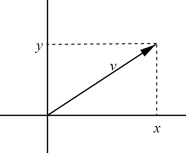
Figure 1.1: An element \(v=(x,y)\) in \(\mathbb{R}^2\) represented by a vector in the plane.
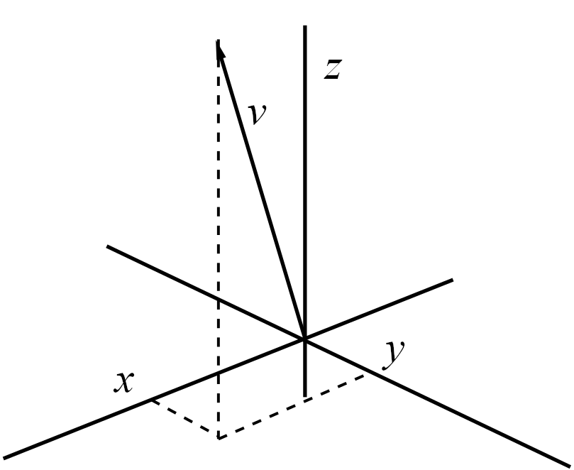
Figure 1.2: An element \(v=(x,y)\) in \(\mathbb{R}^3\) represented by a vector in the plane. Note the positioning of the axes relative to one another in 3D: this is the convention we follow and \(x\) and \(y\) should not be switched (as the their relative positions have consequences for later results).
We define two key operations on vectors, addition and scalar multiplication.
We may refer to the addition as ‘component-wise’, meaning that we are performing the operation of addition on each component individually. Note that we are not defining multiplication of two vectors here: we are multiplying a vector \(x\) by a scalar \(\lambda\).
A simple consequence of the definition is that scalar multiplication is distributive over addition. This means that for any \(x,y\in\mathbb{R}^n\) and \(\lambda\in\mathbb{R}\) \[\lambda(x+y)=\lambda x+\lambda y.\]
By further combining the above operations we can form expressions like \(\lambda v+\mu w\) for \(v,w\in\mathbb{R}^n\) and \(\lambda,\mu\in \mathbb{R}\). We call this a linear combination of \(v\) and \(w\).
We can also consider linear combinations of \(k\) vectors \(v_1, v_2, \cdots ,v_k\in \mathbb{R}^n\) with coefficients \(\lambda_1, \lambda_2\cdots,\lambda_k\in\mathbb{R}\), \[\lambda_1v_1+\lambda_2v_2+\cdots +\lambda_kv_k=\sum_{i=1}^k\lambda_iv_i\]
Notice that \(0v=(0, 0, \dots, 0)\) for any \(v\in\mathbb{R}^n\) and we will denote the vector whose entries are all \(0\) by \(\mathbf{0}\), so we have \[v+\mathbf{0}=\mathbf{0}+v=v\] for any \(v\in\mathbb{R}^n\). Note that when we say \(0v=\mathbf{0}\), the \(0\) on the left hand side is \(0\in\mathbb{R}\), whereas the \(\mathbf{0}\) in the right hand side is \(\mathbf{0}=(0,0, \cdots ,0)\in\mathbb{R}^n\). We use the notation \(\mathbf{0}\) to represent the zero vector regardless of \(n\), but the length of the vector should be clear from the context.
For any \(v \in \mathbb{R}^n\) we have that \(v+(-1)v=0\) and so \((-1)v=-v\). We write \[ w- v:= w+(-1) v.\]
Addition and negative vectors can also be pictured in two and three dimensions, as shown in Figure 1.3 for the \(\mathbb{R}^2\) setting.
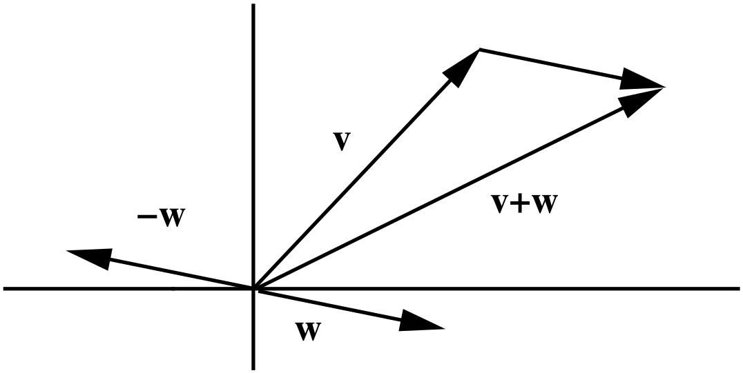
Figure 1.3: Vector addition \(v+w\), and the negative \(-w\).
Before moving on to look at further properties of our vectors we introduce some notation for some vectors which will come up frequently during the course.