Chapter 11 Linear mixed models for more than two measurements
11.1 Pre-mid-post intervention designs
library(tidyverse)
library(knitr)
library(broom)
library(lmerTest)
In many intervention studies, one has more than two measurement moments. Let’s go back to the example of the effect of aspirin on headache in Chapter ??. Suppose you’d like to know whether there is not only a short-term effect of aspirin, but also a long-term effect. Imagine that the study on headache among NY Times readers was extended by asking patients not only to rate their headache before aspirin and 3 hours after intake, but also 24 hours after intake. In this case our data could look like as presented in Table 11.1.
| patient | pre | post1 | post2 |
|---|---|---|---|
| 1 | 52 | 45 | 47 |
| 2 | 59 | 50 | 55 |
| 3 | 65 | 56 | 58 |
| 4 | 51 | 37 | 42 |
| 5 | 62 | 50 | 55 |
| 6 | 61 | 53 | 57 |
| 7 | 56 | 44 | 55 |
| 8 | 62 | 48 | 53 |
| 9 | 56 | 48 | 49 |
| 10 | 58 | 45 | 44 |
So for each patient we have three measures: pre, post1 and post2.
To see if there is some clustering, it is no longer possible to study
this by computing a single correlation. We could however compute 3
different correlations: pre-post1, pre-post2, and
post1-post2, but this is rather tedious, and moreover does not give
us a single measure of the extent of clustering of the data. But there
is an alternative: one could compute not a Pearson correlation, but an
intraclass correlation (ICC). To do this, we need to bring the data
again into long format, as opposed to wide format, see Chapter 1. This is
done in Table 11.2.
| patient | measure | headache |
|---|---|---|
| 1 | pre | 52 |
| 1 | post1 | 45 |
| 1 | post2 | 47 |
| 2 | pre | 59 |
| 2 | post1 | 50 |
| 2 | post2 | 55 |
| 3 | pre | 65 |
| 3 | post1 | 56 |
| 3 | post2 | 58 |
| 4 | pre | 51 |
Next, we can perform an analysis with the lmer() function from the
lme4 package.
library(lme4)
model1 <- datalong %>%
  lmer(headache ~ measure + (1|patient), data = ., REML = FALSE)
model1
## Linear mixed model fit by maximum likelihood ['lmerMod']
## Formula: headache ~ measure + (1 | patient)
## Data: .
## AIC BIC logLik deviance df.resid
## 1740.998 1759.517 -865.499 1730.998 295
## Random effects:
## Groups Name Std.Dev.
## patient (Intercept) 5.290
## Residual 2.908
## Number of obs: 300, groups: patient, 100
## Fixed Effects:
## (Intercept) measurepost2 measurepre
## 49.32 2.36 9.85In the output we see the fixed effects of two automatically created
dummy variables measurepost2 and measurepre, and the intercept. We
also see the standard deviations of the random effects: the standard
deviation of the residuals and the standard deviation of the random
effects for the patients.
From this output, we can plug in the values into the equation:
\[\begin{aligned} \texttt{headache}_{ij} &= 49.32 + patient_i + 2.36 \; \texttt{measurepost2} + 9.85 \; \texttt{measurepre} + e_{ij} \nonumber\\ patient_i &\sim N(0, \sigma_p = 5.29 )\nonumber\\ e_{ij} &\sim N(0, \sigma_e = 2.91)\nonumber\end{aligned}\]
Based on this equation, the expected headache severity score in the
population three hours after aspirin intake is 49.32 (the first post
measure is the reference group). Dummy variable measurepost2 is coded
1 for the measurements 24 hours after aspirin intake. Therefore, the
expected headache score 24 hours after aspirin intake is equal to
\(49.32 + 2.36 = 51.68\). Dummy variable measurepre was coded 1 for the
measurements before aspirin intake. Therefore, the expected headache
before aspirin intake is equal to \(49.32 + 9.85 = 59.17\). In sum, in
this sample we see that the average headache level decreases directly
after aspirin intake from 59.17 to 49.32, but then increases again to
51.68.
There is quite some variation in individual headache levels: the
variance is equal to \(5.29 ^2 = 27.98\), since the standard deviation
(its square root) is equal to 5.29. Therefore, if we look at roughly 95%
of the sample, we see that prior to taking aspirin, the scores vary
between \(59.17 - 2\times 5.29 = 48.59\) and
\(59.17 + 2 \times 5.29 = 69.75\). For the short-term effect of aspirin
after 3 hours, we see that roughly 95% of the scores lie between
\(49.32 -2\times 5.29 = 38.74\) and \(49.32 + 2 \times 5.29 = 59.90\). The
normal distributions, predicted by this model, are depicted in Figure
11.1.
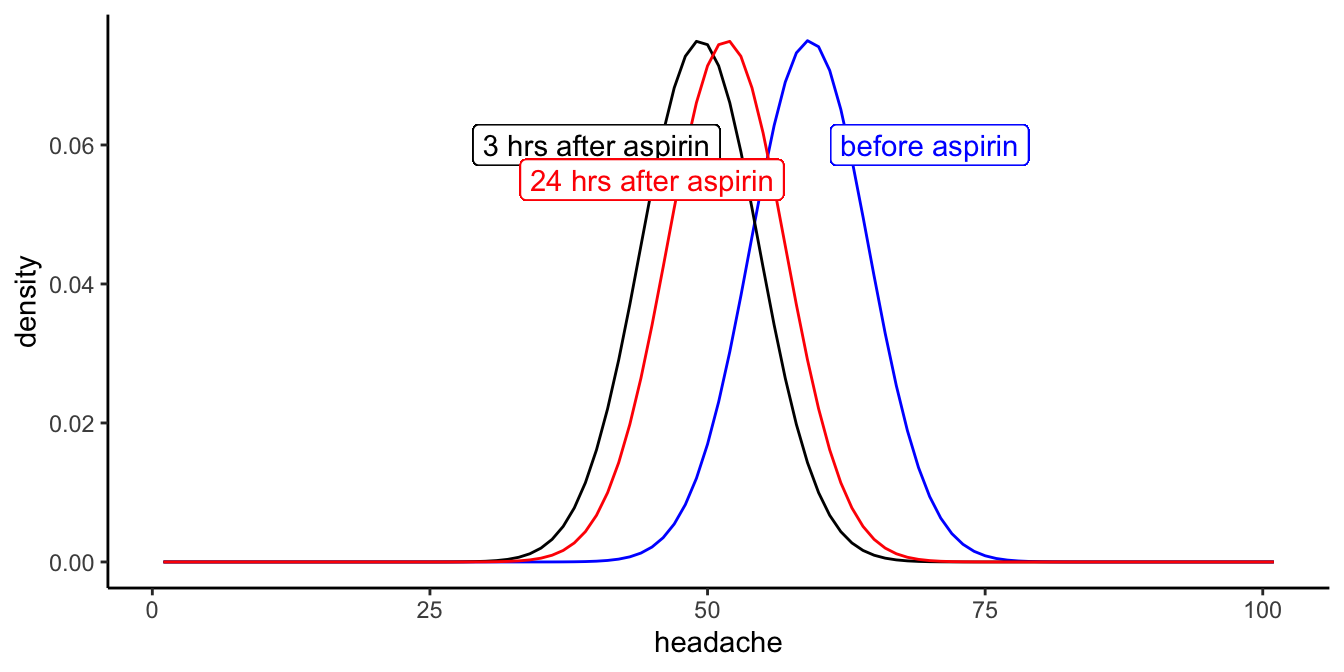
Figure 11.1: Distributions of the three headache levels before aspirin intake, 3 hours after intake and 24 hours after intake, according to the linear mixed model.
So, are these distributions significantly different, in other words, do the means differ significantly before aspirin, 3 hrs after aspirin and 24 hrs after aspirin?
To answer a question about the equality of three means, we need an analysis of variance (ANOVA).
model1 %>% anova()## Analysis of Variance Table
## npar Sum Sq Mean Sq F value
## measure 2 5289.7 2644.9 312.71The \(F\)-statistic for the equality of the group means is quite large
(remember that the expected value is always 1 if the null-hypothesis is
true, see Chapter 6). We see no degrees of freedom. These need
to be estimated, for example using Satterthwaite’s method, provided by
the lmerTest package:
library(lmerTest)##
## Attaching package: 'lmerTest'## The following object is masked from 'package:lme4':
##
## lmer## The following object is masked from 'package:stats':
##
## stepmodel2 <- datalong %>%
lmer(headache ~ measure + (1|patient),
data = .,
REML = FALSE)
model2 %>% anova()## Type III Analysis of Variance Table with Satterthwaite's method
## Sum Sq Mean Sq NumDF DenDF F value Pr(>F)
## measure 5289.7 2644.9 2 200 312.71 < 0.00000000000000022 ***
## ---
## Signif. codes: 0 '***' 0.001 '**' 0.01 '*' 0.05 '.' 0.1 ' ' 1Using Satterthwaite’s method, we see that the error degrees of freedom is 200. The model degrees of freedom is of course 2, because we needed two dummy variables for the three measurements. The \(p\)-value associated with the \(F\)-value of 312.71 at 2 and 200 degrees of freedom is less than 0.05, so we can reject the null-hypothesis. Thus we can report:
"The null-hypothesis that the mean headache level does not change over time was tested with a linear mixed model, with measure entered as a fixed categorical effect ("before", "3hrs after", "24 hrs after") and random effects for patient. An ANOVA showed that the null-hypothesis could be rejected, \(F(2, 200) = 312.71, p < .001\)."
If one has specific hypotheses regarding short-term and long-term
effects, one could perform a planned contrast analysis (see Chapter
7, forthcoming), comparing the first measure
with the second measure, and the first measure with the third measure.
If one is just interested in whether aspirin has an effect on headache,
then the overall \(F\)-test should suffice. If apart from this general
effect one wishes to explore whether there are significant differences
between the three groups of data, without any prior research hypothesis
about this, then one could perform a post hoc analysis of the three
means. See Chapter
7 (forthcoming) on how to perform planned
comparisons and post hoc tests.
Now recall that we mentioned an intraclass correlation, or ICC. An
intraclass correlation indicates how much clustering there is within the
groups, in this case, clustering of headache scores within individual NY
Times readers. How much are the three scores alike that come from the
same patient? This correlation can be computed using the following
formula:
\[\begin{aligned} ICC = \frac{\sigma^2_{patient} } {\sigma^2_{patient} +\sigma^2_e } \end{aligned}\]
Here, the variance of the patient random effects is equal to
\(5.29^2 = 27.98\), and the variance of the residuals \(e\) is equal to
\(2.91^2 = 8.47\), so the intraclass correlation for the headache severity
scores is equal to
\[\begin{aligned} ICC = \frac{27.98} {27.98 + 8.47 } = 0.77 \end{aligned}\]
As this correlation is substantially higher than 0, we conclude there is
quite a lot of clustering. Therefore it’s a good thing that we used
random effects for the individual differences in headache scores among
NY Times readers. Had this correlation been 0 or very close to 0,
however, then it would not have mattered to include these random
effects. In that case, we might as well use an ordinary linear model,
using the lm() function. Note from the formula that the correlation
becomes 0 when the variance of the random effects for patients is 0. It
approaches 0 as the random effects for patients grows small relative to
the residual variance. It approaches 1 as the random effects for
patients grows large relative to the residual variance. Because variance
cannot be negative, ICCs always have values between 0 and 1.
When is an ICC large and when is it small? This is best thought of as being at a birthday party. Most birthday cakes are intended for 8 to 12 guests. If you therefore have one tenth of a birthday cake, that’s a substantial piece. It will most likely fill you up. Therefore, an ICC of 0.10 is definitely to be reckoned with. A larger piece than the regular size will fill you up for the rest of the day. A somewhat smaller piece, say 0.05, is also to be taken seriously. It is nice to have a fraction of 0.05 of a whole birthday cake (you don’t mind sharing, do you?). However, when the host offers you one percent of the cake (0.01), at least I would be inclined to say no thank you.
11.2 Pre-mid-post intervention design: linear effects
In the previous section, we’ve looked at categorical variables:
measure ("pre-intervention", "3 hours after", and "24 hours
after"). We can use the same type of analysis for numerical
variables. In fact, we could have used a linear effect for time in the
headache example: using time of measurement as a numeric variable. Let’s
look at the headache data again. But now we’ve created a new variable
time that is based on the variable measure: all first measurements
are coded as time = 0, all second measurements after 3 hours are coded
as time = 3, and all third measurements after 24 hours are coded as
time = 24. Part of the data are presented in Table
11.3.
| patient | measure | headache | time |
|---|---|---|---|
| 1 | pre | 52 | 0 |
| 1 | post1 | 45 | 3 |
| 1 | post2 | 47 | 24 |
| 2 | pre | 59 | 0 |
| 2 | post1 | 50 | 3 |
| 2 | post2 | 55 | 24 |
| 3 | pre | 65 | 0 |
| 3 | post1 | 56 | 3 |
| 3 | post2 | 58 | 24 |
| 4 | pre | 51 | 0 |
Instead of using a categorical intervention variable, with three levels,
we now use a numeric variable, time, indicating the number of hours
that have elapsed after aspirin intake. At point 0 hours, we measure
headache severity, and patients take an aspirin. Next we measure
headache after 3 hours and 24 hours. Above, we wanted to know if there
were differences in average headache between before intake and 3 hrs and
24 hrs after intake. Another question we might ask ourselves: is there a
linear reduction in headache severity after taking aspirin?
For this we can do a linear regression type of analysis. We want to take
into account individual differences in headache severity levels among
patients, so we perform an lmer() analysis, using the following code,
replacing the categorical variable measure by numerical variable
time:
model3 <- datalongnew %>%
  lmer(headache ~ time + (1|patient), data = ., REML = FALSE)
model3
## Linear mixed model fit by maximum likelihood ['lmerModLmerTest']
## Formula: headache ~ time + (1 | patient)
## Data: .
## AIC BIC logLik deviance df.resid
## 1997.2264 2012.0416 -994.6132 1989.2264 296
## Random effects:
## Groups Name Std.Dev.
## patient (Intercept) 4.533
## Residual 5.546
## Number of obs: 300, groups: patient, 100
## Fixed Effects:
## (Intercept) time
## 54.7913 -0.1557In the output we see that the model for our data is equivalent to
\[\begin{aligned} \texttt{headache}_{ij} &= 54.79 + patient_i - 0.1557 \times \texttt{time} + e_{ij} \\ patient_i &\sim N(0, \sigma_p = 4.53)\\ e_{ij} &\sim N(0, \sigma_e = 5.55)\end{aligned}\]
This model predicts that at time 0, the average headache severity score
equals 54.79, and that for every hour after intake, the headache level
drops by 0.1557 points. So it predicts for example that after 10 hours,
the headache has dropped 1.557 points to 53.23.
Is this a good model for the data? Probably not. Look at the variance of
the residuals: with a standard deviation of 5.55 it is now a lot bigger
than in the previous analysis with the same data (see previous section).
Larger variance of residuals means that the model explains the data
worse: predictions are worse, so the residuals increase in size.
That the model is not appropriate for this data set is also obvious when
we plot the data, focusing on the relationship between time and
headache levels, see Figure
11.2.
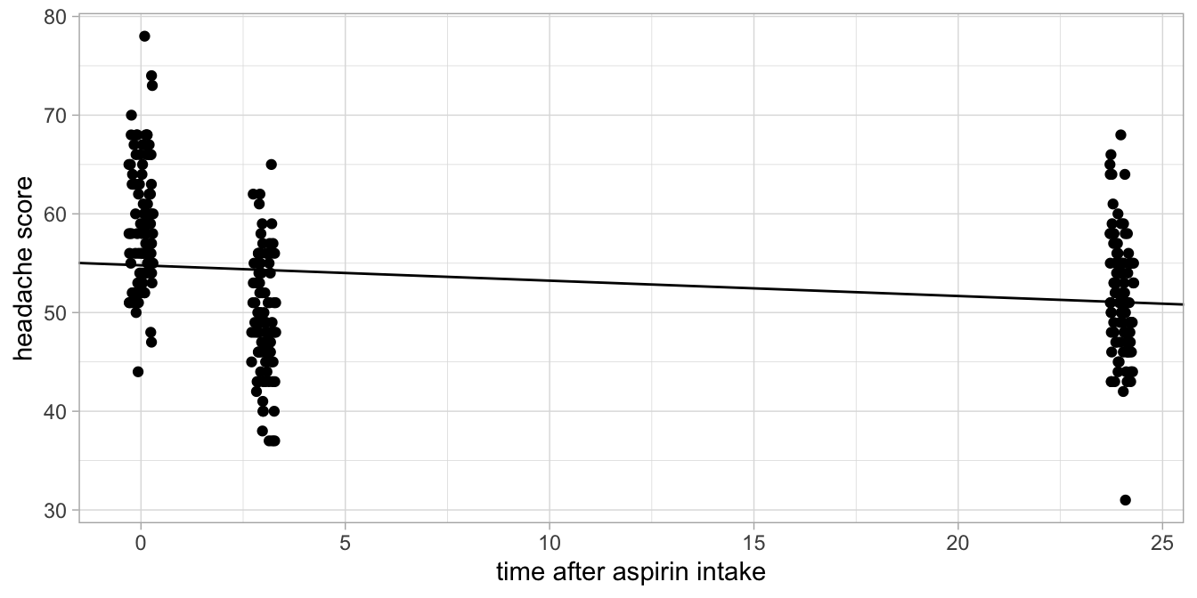
Figure 11.2: Headache levels before aspirin intake, 3 hours after intake and 24 hours after intake.
The line shown is the fitted line based on the output. It can be seen
that the prediction for time = 0 is systematically too low, for
time = 3 systematically too high, and for time = 24 again too low.
So for this particular data set on headache, it would be better to use a
categorical predictor for the effect of time on headache, like we did in
the previous section.
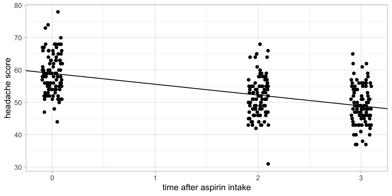
Figure 11.3: Alternative headache levels before aspirin intake, 3 hours after intake and 24 hours after intake.
As an example of a data set where a linear effect would have been appropriate, imagine that we measured headache 0 hours, 2 hours and 3 hours after aspirin intake (and not after 24 hours). Suppose these data would look like those in Figure 11.3. There we see a gradual increase of headache levels right after aspirin intake. Here, a numeric treatment of the time variable would be quite appropriate.
Suppose we would then see the following output.
model4 <- datalongnew2 %>%
  lmer(headache ~ time + (1|patient), data = ., REML = FALSE)
model4 %>% summary()
## Linear mixed model fit by maximum likelihood . t-tests use Satterthwaite's
## method [lmerModLmerTest]
## Formula: headache ~ time + (1 | patient)
## Data: .
##
## AIC BIC logLik deviance df.resid
## 1745.4 1760.2 -868.7 1737.4 296
##
## Scaled residuals:
## Min 1Q Median 3Q Max
## -2.78967 -0.55395 0.05095 0.56015 2.30971
##
## Random effects:
## Groups Name Variance Std.Dev.
## patient (Intercept) 27.889 5.281
## Residual 8.732 2.955
## Number of obs: 300, groups: patient, 100
##
## Fixed effects:
## Estimate Std. Error df t value Pr(>|t|)
## (Intercept) 58.9721 0.6000 134.6807 98.29 <0.0000000000000002 ***
## time -3.3493 0.1368 200.0000 -24.48 <0.0000000000000002 ***
## ---
## Signif. codes: 0 '***' 0.001 '**' 0.01 '*' 0.05 '.' 0.1 ' ' 1
##
## Correlation of Fixed Effects:
## (Intr)
## time -0.380Because we are confident that this model is appropriate for our data, we can interpret the statistical output. The Satterthwaite error degrees of freedom are 200, so we can construct a 95% confidence interval by finding the appropriate \(t\)-value.
qt(0.975, df = 200)## [1] 1.971896The 95% confidence interval for the effect of time is then from \(-3.349 - 1.97 \times 0.1368\) to \(-3.349 + 1.97 \times 0.1368\), so from -3.62 to -3.08. We can report:
"A linear mixed model was run on the headache levels, using a fixed effect for the numeric predictor variable time and random effects for the variable patient. We saw a significant linear effect of time on headache level, \(t(200)=-24.42, p < .001\). The estimated effect of time based on this analysis is negative, \(-3.35\), so with every hour that elapses after aspirin intake, the predicted headache score decreases with 3.35 points (95% CI: 3.08 to 3.62 points)".
11.3 Linear mixed models and interaction effects
Suppose we carry out the aspirin and headache study not only with a
random sample of NY Times readers that suffer from regular headaches,
but also with a random sample of readers of the Wall Street Journal that
suffer from regular headaches. We’d like to know whether aspirin works,
but we are also interested to know whether the effect of aspirin is
similar in the two groups of readers. Our null-hypothesis is that the
effect of aspirin in affecting headache severity is the same in NY Times
and Wall Street Journal readers that suffer from headaches.
\(H_0\): The effect of aspirin is the same for NY Times readers as for
Wall Street Journal readers.
Suppose we have the data set in Table
11.4 (we only show the first six
patients), and we only look at the measurements before aspirin intake
and 3 hours after aspirin intake (pre-post design).
| patient | group | pre | post |
|---|---|---|---|
| 1 | NYTimes | 55 | 45 |
| 2 | WallStreetJ | 63 | 50 |
| 3 | NYTimes | 66 | 56 |
| 4 | WallStreetJ | 50 | 37 |
| 5 | NYTimes | 63 | 50 |
| 6 | WallStreetJ | 65 | 53 |
In this part of the data set, patients 2, 4, and 6 read the Wall Street
Journal, and patients 1, 3 and 5 read the NY Times. We assume that
people only read one of these newspapers. We measure their headache
before and after the intake of aspirin (a pre-post design). The data are
now in what we call wide format: the dependent variable headache is
spread over two columns, pre and post. In order to analyse the data
with linear models, we need them in long format, as in Table
11.5.
| patient | group | measure | headache |
|---|---|---|---|
| 1 | NYTimes | pre | 55 |
| 1 | NYTimes | post | 45 |
| 2 | WallStreetJ | pre | 63 |
| 2 | WallStreetJ | post | 50 |
| 3 | NYTimes | pre | 66 |
| 3 | NYTimes | post | 56 |
datalong <- datawide %>%
  pivot_longer(cols = -c(patient, group),
               names_to = "measure",
               values_to = "headache")
The new variable measure now indicates whether a given measurement of
headache refers to a measurement before intake (pre) or after intake
(post). Again we could investigate whether there is an effect of aspirin
with a linear mixed model, with measure as our categorical predictor,
but that is not really what we want to test: we only want to know
whether the effect of aspirin (being small, large, negative or
non-existent) is the same for both groups. Remember that this
hypothesis states that there is no interaction effect of aspirin
(measure) and group. The null-hypothesis is that group is not a
moderator of the effect of aspirin on headache. There may be an effect
of aspirin or there may not, and there may be an effect of newspaper
(group) or there may not, but we’re interested in the interaction of
aspirin and group membership. Is the effect of aspirin different for NY
Times readers than for Wall Street Journal readers?
In our model we therefore need to specify an interaction effect. Since
the data are clustered (2 measures per patient), we use a linear mixed
model. First we show how to analyse these data using dummy variables,
later we will show the results using a different approach.
We recode the data into two dummy variables, one for the aspirin
intervention (dummy1: 1 if measure = post, 0 otherwise), and one for
group membership (dummy2: 1 if group = NYTimes, 0 otherwise):
datalong <- datalong %>%
  mutate(dummy1 = ifelse(measure == "post", 1, 0),
         dummy2 = ifelse(group == "NYTimes", 1, 0))
datalong %>% head(3)
## # A tibble: 3 x 6
## patient group measure headache dummy1 dummy2
## <int> <chr> <chr> <dbl> <dbl> <dbl>
## 1 1 NYTimes pre 55 0 1
## 2 1 NYTimes post 45 1 1
## 3 2 WallStreetJ pre 63 0 0Next we need to compute the product of these two dummies to code a dummy for the interaction effect. Since with the above dummy coding, all post measures get a 1, and all NY Times readers get a 1, only the observations that are post aspirin and that are from NY Times readers get a 1 for this product.
datalong <- datalong %>%
  mutate(dummy_interact = dummy1*dummy2)
datalong %>% head(3)
## # A tibble: 3 x 7
## patient group measure headache dummy1 dummy2 dummy_interact
## <int> <chr> <chr> <dbl> <dbl> <dbl> <dbl>
## 1 1 NYTimes pre 55 0 1 0
## 2 1 NYTimes post 45 1 1 1
## 3 2 WallStreetJ pre 63 0 0 0With these three new dummy variables we can specify the linear mixed model.
model5 <- datalong %>%
  lmer(headache ~ dummy1 + dummy2 + dummy_interact + (1|patient),
       data = .,
       REML = FALSE)
model5
## Linear mixed model fit by maximum likelihood ['lmerModLmerTest']
## Formula: headache ~ dummy1 + dummy2 + dummy_interact + (1 | patient)
## Data: .
## AIC BIC logLik deviance df.resid
## 1201.6855 1221.4754 -594.8427 1189.6855 194
## Random effects:
## Groups Name Std.Dev.
## patient (Intercept) 5.177
## Residual 2.855
## Number of obs: 200, groups: patient, 100
## Fixed Effects:
## (Intercept) dummy1 dummy2 dummy_interact
## 59.52 -10.66 0.32 0.60In the output, we recognise the three fixed effects for the three dummy
variables. Since we’re interested in the interaction effect, we look at
the effect of dummy_interact. The effect is in the order of +0.6. What
does this mean?
Remember that all headache measures before aspirin intake are given a 0
for the intervention dummy dummy1. A reader from the Wall Street
Journal gets a 0 for the group dummy dummy2. Since the product of
\(0\times 0\) equals 0, all measures before aspirin in Wall Street Journal
readers get a 0 for the interaction dummy dummy_interact. Therefore,
the intercept of 59.52 refers to the expected headache severity of Wall
Street Journal readers before they take their aspirin.
Furthermore, we see that the effect of dummy1 is -10.66. The variable
dummy1 codes for post measurements. So, relative to Wall Street
Journal readers prior to aspirin intake, the level of post intake
headache is 10.66 points lower.
If we look further in the output, we see that the effect of dummy2
equals +0.32. This variable dummy2 codes for NY Times readers. So,
relative to Wall Street Journal readers and before aspirin intake (the
reference group), NY Times readers score on average 0.32 points higher
on the headache scale.
However, we’re not interested in a general difference between those two groups of readers, we’re interested in the effect of aspirin and whether it is different in the two groups of readers. In the output we see the interaction effect: being a reader of the NY Times AND at the same time being a measure after aspirin intake, the expected level of headache is an extra +0.60. The effect of aspirin is -10.66 in Wall Street Journal readers, as we saw above, but the effect is \(-10.66 + 0.60 = -10.06\) in NY Times readers. So in this sample the effect of aspirin on headache is 0.60 smaller than in Wall Street Journal readers (note that even while the interaction effect is positive, it is positive on a scale where a high score means more headache).
Let’s look at it in a different way, using a table with the dummy codes, see Table ??. For each group of data, pre or post aspirin and NY Times readers and Wall Street Journal readers, we note the dummy codes for the new dummy variables. In the last column we use the output estimates and multiply them with the respective dummy codes (1 and 0) to obtain the expected headache level (using rounded numbers):
| measure | group | dummy1 | dummy2 | dummy_interact | exp mean |
|---|---|---|---|---|---|
| pre | WallStreetJ | 0 | 0 | 0 | \(60\) |
| post | WallStreetJ | 1 | 0 | 0 | \(60 + (-11)=49\) |
| pre | NYTimes | 0 | 1 | 0 | \(60 + 0.3=60.3\) |
| post | NYTimes | 1 | 1 | 1 | \(60 +(-11) + 0.3 + 0.6=49.9\) |
{#tab:exp label=“tab:exp”}
The exact numbers are displayed in Figure 11.4.
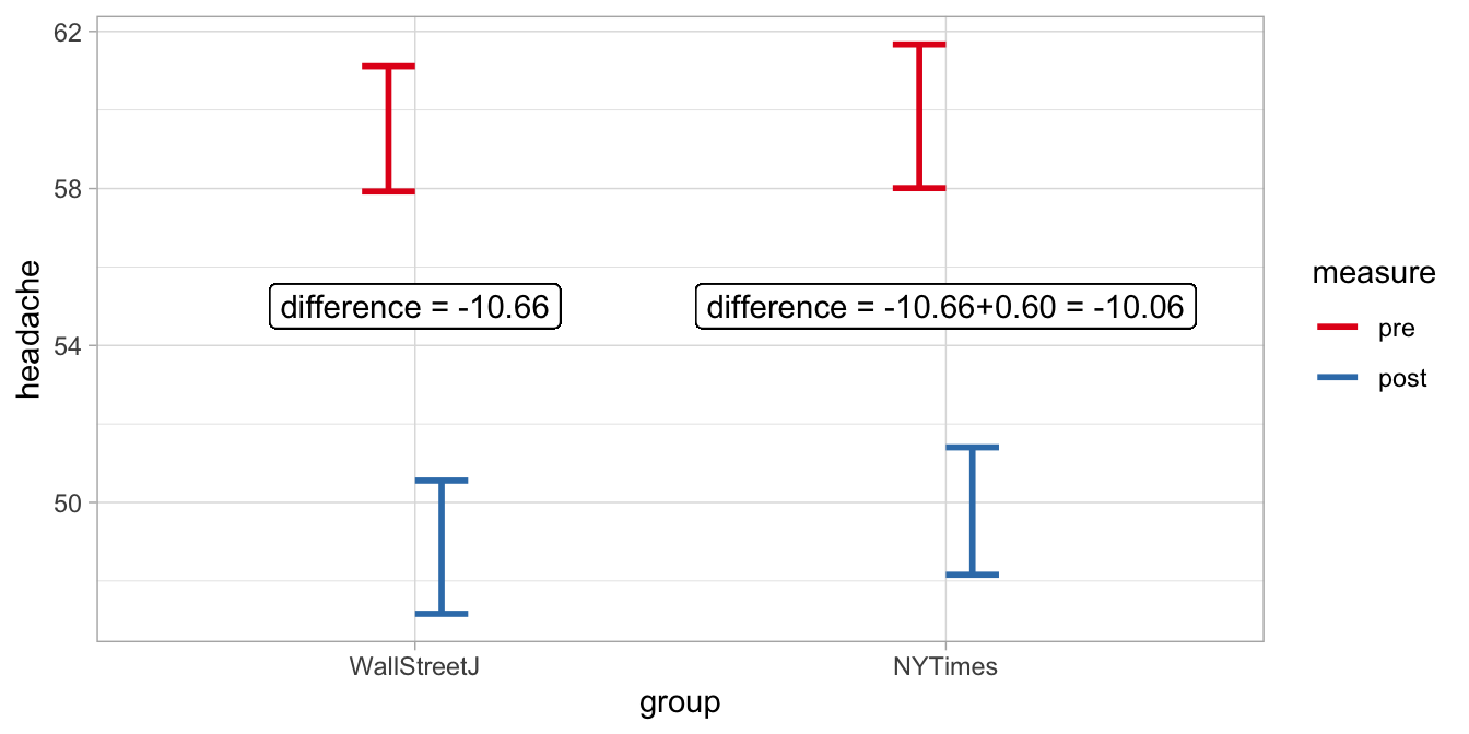
Figure 11.4: Expected headache levels in NY Times readers and Wall Street Journal readers based on a linear mixed model with an interaction effect.
We see that the specific effect of aspirin in NY Times readers is 0.60 smaller than the effect of aspirin in Wall Street Journal readers. This difference in the effect of aspirin between the groups was not significantly different from 0, as we can see when we let R plot a summary of the results.
model5 %>% summary()## Linear mixed model fit by maximum likelihood . t-tests use Satterthwaite's
## method [lmerModLmerTest]
## Formula: headache ~ dummy1 + dummy2 + dummy_interact + (1 | patient)
## Data: .
##
## AIC BIC logLik deviance df.resid
## 1201.7 1221.5 -594.8 1189.7 194
##
## Scaled residuals:
## Min 1Q Median 3Q Max
## -2.34085 -0.43678 -0.02942 0.50880 2.22534
##
## Random effects:
## Groups Name Variance Std.Dev.
## patient (Intercept) 26.80 5.177
## Residual 8.15 2.855
## Number of obs: 200, groups: patient, 100
##
## Fixed effects:
## Estimate Std. Error df t value Pr(>|t|)
## (Intercept) 59.5200 0.8361 125.9463 71.192 <0.0000000000000002 ***
## dummy1 -10.6600 0.5710 100.0000 -18.670 <0.0000000000000002 ***
## dummy2 0.3200 1.1824 125.9463 0.271 0.787
## dummy_interact 0.6000 0.8075 100.0000 0.743 0.459
## ---
## Signif. codes: 0 '***' 0.001 '**' 0.01 '*' 0.05 '.' 0.1 ' ' 1
##
## Correlation of Fixed Effects:
## (Intr) dummy1 dummy2
## dummy1 -0.341
## dummy2 -0.707 0.241
## dummy_ntrct 0.241 -0.707 -0.341"The null-hypothesis that the effect of aspirin is the same in the two populations of readers cannot be rejected, \(t(100)=0.743, p = .46\). We therefore conclude that there is no evidence that aspirin has a different effect for NY Times than for Wall Street Journal readers."
Note that we could have done the analysis in another way, not recoding
the variables into numeric dummy variables ourselves, but by letting R
do it automatically. R does that automatically for factor variables like
our variable group. The code is then:
model6 <- datalong %>%
  lmer(headache ~ measure + group + measure:group + (1|patient),
       data = .,
       REML = FALSE)
model6 %>% summary()
## Linear mixed model fit by maximum likelihood . t-tests use Satterthwaite's
## method [lmerModLmerTest]
## Formula: headache ~ measure + group + measure:group + (1 | patient)
## Data: .
##
## AIC BIC logLik deviance df.resid
## 1201.7 1221.5 -594.8 1189.7 194
##
## Scaled residuals:
## Min 1Q Median 3Q Max
## -2.34085 -0.43678 -0.02942 0.50880 2.22534
##
## Random effects:
## Groups Name Variance Std.Dev.
## patient (Intercept) 26.80 5.177
## Residual 8.15 2.855
## Number of obs: 200, groups: patient, 100
##
## Fixed effects:
## Estimate Std. Error df t value
## (Intercept) 49.7800 0.8361 125.9463 59.542
## measurepre 10.0600 0.5710 100.0000 17.619
## groupWallStreetJ -0.9200 1.1824 125.9463 -0.778
## measurepre:groupWallStreetJ 0.6000 0.8075 100.0000 0.743
## Pr(>|t|)
## (Intercept) <0.0000000000000002 ***
## measurepre <0.0000000000000002 ***
## groupWallStreetJ 0.438
## measurepre:groupWallStreetJ 0.459
## ---
## Signif. codes: 0 '***' 0.001 '**' 0.01 '*' 0.05 '.' 0.1 ' ' 1
##
## Correlation of Fixed Effects:
## (Intr) mesrpr grpWSJ
## measurepre -0.341
## grpWllStrtJ -0.707 0.241
## msrpr:grWSJ 0.241 -0.707 -0.341R has automatically created dummy variables, one dummy measurepre that
codes 1 for all measurements before aspirin intake, one dummy
groupWallStreetJ that codes 1 for all measurements from Wall Street
Journal readers, and one dummy measurepre:groupWallStreetJ that codes
1 for all measurements from Wall Street Journal readers before aspirin
intake. Because the dummy coding is different from the hand coding we
did ourselves earlier, the intercept and the main effects of group and
measure are now different. We also see that the significance level of
the interaction effect is still the same. You are always free to choose
to either construct your own dummy variables and analyse them in a
quantitative way (using numeric variables), or to let R construct the
dummy variables for you (by using a factor variable): the \(p\)-value for
the interaction effect will always be the same (this is not true for the
intercept and the main effects).
Because the two analyses are equivalent (they end up with exactly the same predictions, feel free to check!), we can safely report that we have found a non-significant group by measure interaction effect, \(t(100)=0.74, p = .46\). We therefore conclude that we found no evidence that in the populations of NY Times readers and Wall Street Journal readers, the short-term effect of aspirin on headache is any different.
11.4 Mixed designs
The design in the previous section, where we had both a grouping
variable and a pre-post or repeated measures design, is often called a
mixed design. It is a mixed design in the sense that there are two
kinds of variables: one is a between-individuals variable, and one
variable is a within-individual variable. Here the between-individuals
variable is group: two different populations of readers. It is called
between because one individual can only be part of one group. When we
study the effect of the group effect we are essentially comparing the
scores of one group of individuals with the scores of another group of
individuals, so the comparison is between different individuals. The
two groups of data are said to be independent, as we knew that none of
the readers in this data set reads both journals.
The within-variable in this design is the aspirin intervention,
indicated by the variable measure. For each individual we have two
observations: all individuals are present in both the pre condition data
as well as in the post condition data. With this intervention variable,
we are comparing the scores of a group of individuals with the scores
of that same group of individuals at another time point. The
comparison of scores is within a particular individual, at time point 1
and at time point 2. So the pre and post sets of data are not
independent: the headache scores in both conditions are coming from the
same individuals.
Mixed designs are often seen in psychological experiments. For instance, you want to know how large the effect of alcohol intake is on driving performance. You want to know whether the effect of alcohol on driving performance is the same in a Fiat 600 as in a Porsche 918. Suppose you have 100 participants for your study. There are many choices you can make regarding the design of your study. Here we discuss 4 alternative research designs:
One option is to have all participants participate in all four conditions: they all drive a Fiat with and without alcohol, and they all drive a Porsche, with and without alcohol. In this case, both the car and the alcohol are within-participant variables.
The second option is to have 50 participants drive a Porsche, with and without alcohol, and to have the other 50 participants drive the Fiat, with and without alcohol. In this case, the car is the between-participants variable, and alcohol is the within-participant variable.
The third option is to have 50 participants without alcohol drive both the Porsche and the Fiat, and to have the other 50 participants drive the Porsche and the Fiat with alcohol. Now the car is the within-participant variable, and the alcohol is the between-participants variable.
The fourth option is to have 25 participants drive the Porsche with alcohol, 25 other participants drive the Porsche without alcohol, 25 participants drive the Fiat with alcohol, and the remaining 25 participants drive the Fiat without alcohol. Now both the car variable and the alcohol variable are between-participant variables: none of the participants is present in more than 1 condition.
Only the second and the third design described here are mixed designs, having at least one between-participants variable and at least one within-participant variable.
Remember that when there is at least one within variable in your design, you have to use a linear mixed model. If all variables are between variables, one can use an ordinary linear model. Note that the term mixed in linear mixed model refers to the effects in the model that can be both random and fixed. The term mixed in mixed designs refers to the mix of two kinds of variables: within variables and between variables.
Also note that the within and between distinction refers to the units of analysis. If the unit of analysis is school, then the denomination of the school is a between-school variable. An example of a within-school variable could be time: before a major curriculum reform and after a major curriculum reform. Or it could be teacher: classes taught by teacher A or by teacher B, both teaching at the same school.
11.5 Mixed design with a linear effect
In an earlier section we looked at a mixed design where the between
variable was group and the within variable was measure: pre or post.
It was a 2 by 2 design (\(2 \times 2\)) design: 2 measures and 2 groups,
where we were interested in the interaction effect. We wanted to know
whether group moderated the effect of measure, that is, the effect
of aspirin on headache. We used the categorical within-individual
variable measure in the regression by dummy-coding it.
In an earlier section in this chapter we saw that we can also model linear effects of numeric variables in linear mixed models, where we treated the time variable numerically: 0hrs, 3hrs after aspirin intake and 24 hrs after intake. Here we will give an example of a \(3 \times 20\) mixed design: we have a categorical group (between-individuals) variable with 3 levels and a numeric time (within) variable with 20 levels. The example is about stress in athletes that are going to take part in the 2018 Winter Olympics. Stress can be revealed in morning cortisol levels. In the 20 days preceding the start of the Olympics, each athlete was measured every morning after waking and before breakfast by letting them chew on cotton. The cortisol level in the saliva was then measured in the lab. Our research question is by how much cortisol levels rise in athletes that prepare for the Olympics.
Three groups were studied. One group consisted of 50 athletes who were selected to take part in the Olympics, one group consisted of 50 athletes that were very good but were not selected (Control group I) and one group consisted of 50 non-athlete spectators that were going to watch the games (Control group II). The research question was about what the differences are in average cortisol increase in these three groups: the Olympians, Control group I and Control group II.
In Table 11.6 you see part of the fictional data, the first 6 measurements on person 1 that belongs to the group of Olympians.
| person | group | measure | cortisol |
|---|---|---|---|
| 1 | Olympian | 1 | 19 |
| 1 | Olympian | 2 | 20 |
| 1 | Olympian | 3 | 22 |
| 1 | Olympian | 4 | 23 |
| 1 | Olympian | 5 | 24 |
| 1 | Olympian | 6 | 22 |
When we plot the data, and use different colours for the three different groups, we already notice that the Olympians show generally higher cortisol levels, particularly at the end of the 20-day period (Figure 11.5).
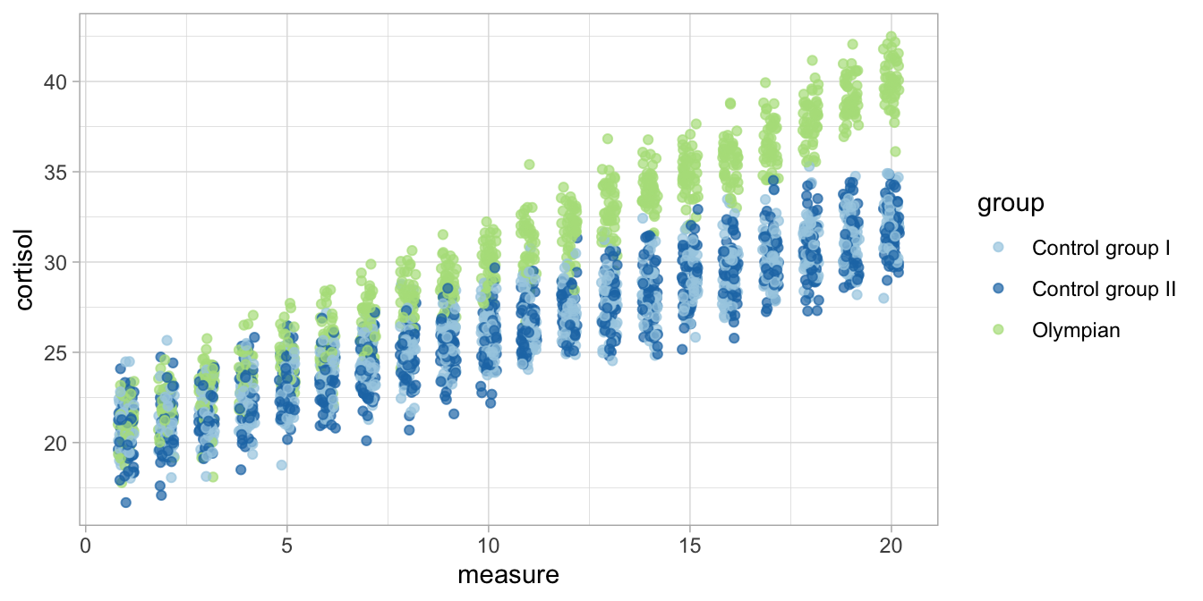
Figure 11.5: Cortisol levels over time in three groups.
We want to know to what extent the linear effect of time is moderated by
group. Since for every person we have 20 measurements, the data are
clustered so we use a linear mixed model. We’re looking for a linear
effect of time, so we use the measure variable numerically (i.e., it
is numeric, and we do not transform it into a factor). We also use the
categorical variable group as a predictor. It is a factor variable
with three levels, so R will automatically make two dummy variables.
Because we’re interested in the interaction effects, we include both
main effects of group and measure as well as their interaction in
the model. Lastly, we control for individual differences in cortisol
levels by introducing random effects for person.
model7 <- datalong %>%
  lmer(cortisol ~ measure + group + measure:group + (1|person),
       data = .,
       REML = FALSE)
model7 %>% summary()
## Linear mixed model fit by maximum likelihood . t-tests use Satterthwaite's
## method [lmerModLmerTest]
## Formula: cortisol ~ measure + group + measure:group + (1 | person)
## Data: .
##
## AIC BIC logLik deviance df.resid
## 8969.8 9017.8 -4476.9 8953.8 2992
##
## Scaled residuals:
## Min 1Q Median 3Q Max
## -3.5823 -0.6405 -0.0116 0.6621 3.3154
##
## Random effects:
## Groups Name Variance Std.Dev.
## person (Intercept) 0.9655 0.9826
## Residual 0.9960 0.9980
## Number of obs: 3000, groups: person, 150
##
## Fixed effects:
## Estimate Std. Error df t value
## (Intercept) 20.094018 0.153650 202.476943 130.778
## measure 0.596989 0.005473 2850.000014 109.078
## groupControl group II -0.226802 0.217293 202.476944 -1.044
## groupOlympian -0.402950 0.217293 202.476944 -1.854
## measure:groupControl group II 0.006383 0.007740 2850.000006 0.825
## measure:groupOlympian 0.411896 0.007740 2850.000006 53.216
## Pr(>|t|)
## (Intercept) <0.0000000000000002 ***
## measure <0.0000000000000002 ***
## groupControl group II 0.2978
## groupOlympian 0.0651 .
## measure:groupControl group II 0.4096
## measure:groupOlympian <0.0000000000000002 ***
## ---
## Signif. codes: 0 '***' 0.001 '**' 0.01 '*' 0.05 '.' 0.1 ' ' 1
##
## Correlation of Fixed Effects:
## (Intr) measur grCgII grpOly m:CgII
## measure -0.374
## grpCntrlgII -0.707 0.264
## groupOlympn -0.707 0.264 0.500
## msr:grpCgII 0.264 -0.707 -0.374 -0.187
## msr:grpOlym 0.264 -0.707 -0.187 -0.374 0.500In the output we see an intercept of 20.09, a slope of about 0.60 for
the effect of measure, two main effects for the variable group
(Control group I is the reference group), and two interaction effects
(one for Control group II and one for the Olympian group). Let’s fill in
the linear model equation based on this output:
\[\begin{aligned} \texttt{cortisol}_{ij} &= 20.09 + person_i + 0.60 \; \texttt{measure} - 0.23 \; \texttt{ContrGrII} - 0.40\; \texttt{Olympian} + \nonumber\\ &0.006 \; \texttt{ContrGrII} \; \texttt{measure} + 0.41 \; \texttt{Olympian} \; \texttt{measure} + e_{ij} \nonumber\\ person_i &\sim N(0, \sigma_p^2 = 0.97)\nonumber\\ e_{ij} &\sim N(0, \sigma_e^2 = 1.00) \nonumber\end{aligned}\]
We see a clear intraclass correlation of around
\(\frac{0.9655}{0.9655+0.9960}= 0.49\) so it’s a good thing we’ve included
random effects for person. The expected means at various time points
and for various groups can be made with the use of the above equation.
It’s aiding interpretation when we look at what linear effects we have for the three different groups. Filling in the above equation for Control group I (the reference group), we get:
\[\begin{aligned} \texttt{cortisol}_{ij} = 20.09 + person_i + 0.60 \times \texttt{measure} + e_{ij} \nonumber\end{aligned}\]
For Control group II we get:
\[\begin{aligned} \texttt{cortisol}_{ij} &= 20.09 + person_i + 0.60 \; \texttt{measure} - 0.23 + 0.006 \; \texttt{measure} + e_{ij} \nonumber \\ &= 19.86 + person_i + 0.606 \times \texttt{measure} + e_{ij} \nonumber\end{aligned}\]
And for the Olympians we get:
\[\begin{aligned} \texttt{cortisol}_{ij} &= 20.09 + person_i + 0.60 \; \texttt{measure} - 0.40 + 0.41 \; \texttt{measure} + e_{ij} \nonumber \\ &= 19.69 + person_i + 1.01 \times \texttt{measure} + e_{ij} \nonumber\end{aligned}\]
In these three equations, all intercepts are close to 20. The slopes are about 0.6 in both Control groups I and II, whereas the slope is around 1 in the group of Olympian athletes. For illustration, these three implied linear regression lines are depicted in Figure 11.6.
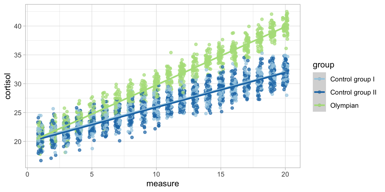
Figure 11.6: Cortisol levels over time in three groups with the group-specific regression lines.
So based on the linear model, we see that in this sample the rise in
cortisol levels is much steeper in Olympians than in the two control
groups. But is this true for all Olympians and the rest of the
populations of high performing athletes and spectators? Note that in the
regression table we see two interaction effects: one for
measure:groupControl group II and one for measure:groupOlympian.
Here we’re interested in the rise in cortisol in the three different
groups and to what extent these sample differences extend to the three
populations.
A possible answer we find in the \(F\)-statistic of an ANOVA. When we run an ANOVA on the results,
model7 %>% anova()## Type III Analysis of Variance Table with Satterthwaite's method
## Sum Sq Mean Sq NumDF DenDF F value Pr(>F)
## measure 54095 54095 1 2850.00 54313.3049 <0.0000000000000002 ***
## group 3 2 2 202.48 1.7285 0.1802
## measure:group 3703 1852 2 2850.00 1859.1587 <0.0000000000000002 ***
## ---
## Signif. codes: 0 '***' 0.001 '**' 0.01 '*' 0.05 '.' 0.1 ' ' 1we see a significant measure by group interaction effect, \(F(2, 2850) = 1859.16, p<.001\). The null-hypothesis of the same cortisol change in three different populations can be rejected, and we conclude that Olympian athletes, non-Olympian athletes and spectators show a different change in cortisol levels in the weeks preceding the games.