Chapter 14 Generalised linear models for count data: Poisson regression
library(lmerTest)
library(tidyverse)
library(knitr)
library(broom)
14.1 Poisson regression
Count data are inherently discrete, and often when using linear models, we see non-normal distributions of residuals. In Chapter 13 we discussed a data set on the scores that a group of students got for an assignment. There were four criteria, and the score consisted of the number of criteria that were met for each student’s assignment. Figure 13.3 showed that after an ordinary linear model analysis, the residuals did not look normal at all.
Table 14.1
shows part of the data that were analysed. The dependent variable was
score. Similar to logistic regression, perhaps we can find a
distribution other than the normal distribution that is more suitable
for this kind of dependent variable? For dichotomous data (1/0) we found
the Bernoulli distribution very useful. For count data like this
variable score, the traditional distribution is the Poisson
distribution.
| ID | score | previous |
|---|---|---|
| 1 | 0 | 0 |
| 2 | 2 | 0 |
| 3 | 4 | 0 |
| 4 | 0 | -1 |
| 5 | 2 | -1 |
| 6 | 3 | 0 |
The normal distribution has two parameters, the mean and the variance. The Bernoulli distribution has only 1 parameter (the probability), and the Poisson distribution has also only 1 parameter, \(\lambda\) (Greek letter ‘lambda.’ \(\lambda\) is a parameter that indicates tendency. Figure 14.1 shows a Poisson distribution with a tendency of 4.
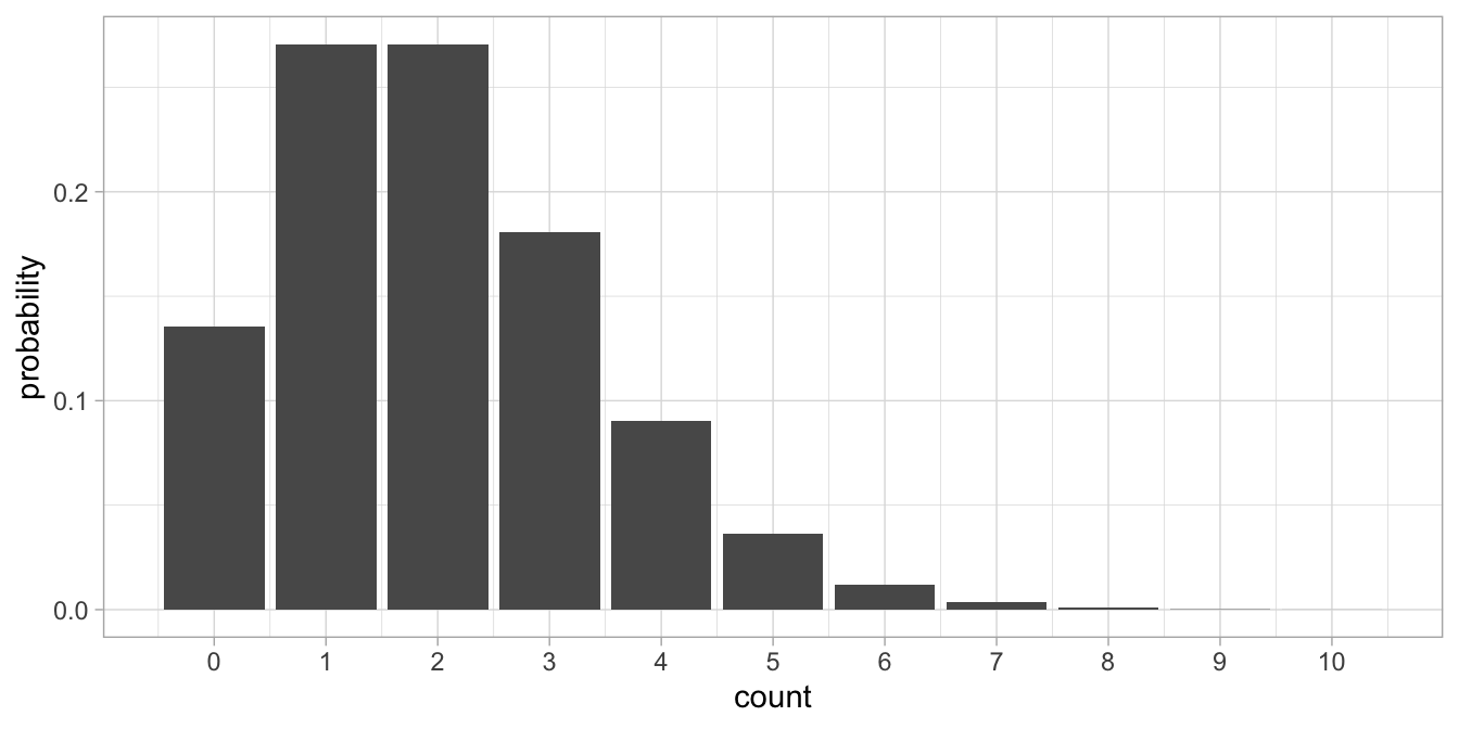
Figure 14.1: Count data example where the normal distribution is not a good approximation of the distribution of the residuals.
What we see is that many values centre around the tendency parameter value of 4 (therefore we call it a tendency parameter). We see only discrete values, and no values below 0. We see a few values higher than 10. If we take the mean of the distribution, we will find a value of 4. If we would compute the variance of the distribution we would also find 4. In general, if we have a Poisson distribution with a tendency parameter \(\lambda\), we know that both the mean and the variance will be equal to \(\lambda\).
A Poisson model could be suitable for our data: a linear equation could predict the parameter \(\lambda\) and then the actual data show a Poisson distribution.
\[\begin{aligned} \lambda &= b_0 + b_1 X \\ Y &\sim Poisson(\lambda)\end{aligned}\]
However, because of the additivity assumption, the equation \(b_0 + b_1 X\) can lead to negative values. A negative value for \(\lambda\) is not logical, because we then have a tendency to observe data like -2 and -4 in our data, which is contrary to having count data, which consists of non-negative integers. A Poisson distribution always shows integers of at least 0, so one way or another we have to make sure that we always have a \(\lambda\) of at least 0.
Remember that we saw the reverse problem with logistic regression: there we wanted to have negative values for our dependent variable logodds ratio, so therefore we used the logarithm. Here we want to have positive values for our dependent variable, so we can use the inverse of the logarithm function: the exponential. Then we have the following model:
\[\begin{aligned} \lambda &= \textrm{exp}(b_0 + b_1 X)= e^{b_0+b_1X} \\ Y &\sim Poisson(\lambda)\end{aligned}\]
This is a generalised linear model, now with a Poisson distribution and an exponential link function. The exponential function makes any value positive, for instance \(\textrm{exp}(0)=1\) and \(\textrm{exp}(-100)=0\).
Let’s analyse the assignment data with this generalised linear model.
Our dependent variable is the number of criteria met for the assignment
(a number between 0 and 4), and the independent variable is previous,
which is a standardised mean of a number of previous assignments. That
means that a student with previous = 0, that student had a mean grade
for previous assignment equal to the mean grade for all students. We
expect that a high mean score on previous assignments is associated with
a higher score on the present assignment. When we run the analysis, the
result is as follows:
\[\begin{aligned} \lambda &= \textrm{exp}(0.1576782 -0.0548685 \times \texttt{previous}) \\ \texttt{score} &\sim Poisson(\lambda)\end{aligned}\]
What does it mean? Well, similar to logistic regression, we can
understand such equations by making some predictions for interesting
values of the independent variable. For instance, a value of 0 for
previous means an average grade on previous assignments that is equal
to the mean of all students. So if we choose previous = 0, then we
have the prediction for an average student. If we fill in that value, we
get the equation
\(\lambda=\textrm{exp}(0.1576782 -0.0548685 \times 0)= \textrm{exp} (0.1576782)= 1.17\).
Thus, for an average student, we expect to see a score of 1.17. A
Poisson distribution with \(\lambda=1.17\) is depicted in Figure
14.2.
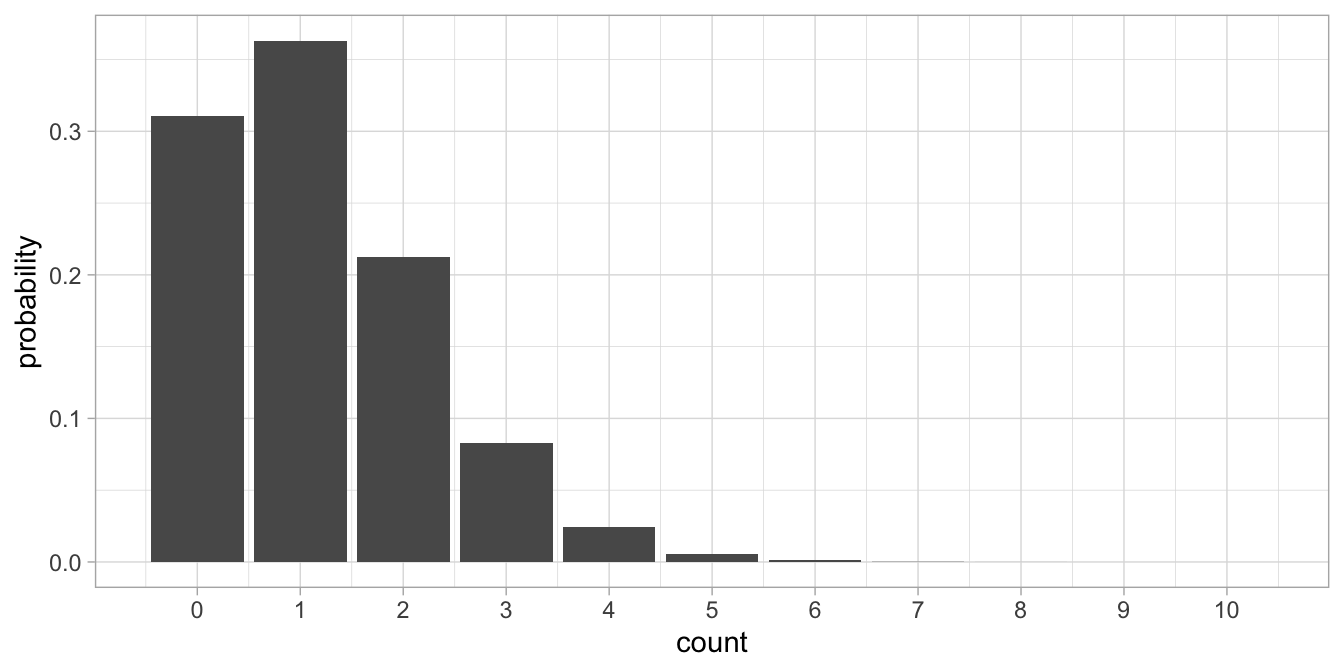
Figure 14.2: Poisson distribution with lambda=1.17.
Another interesting value of previous might be -2. That represents a
student with generally very low grades. Because the average grades were
standardised, only about 2.5% of the students has a lower average grade
than -2. If we fill in that value, we get:
\(\lambda=\textrm{exp}(0.1576782 -0.0548685 \times -2)= 1.31\). A Poisson
distribution with \(\lambda=1.31\) is depicted in Figure
14.3.
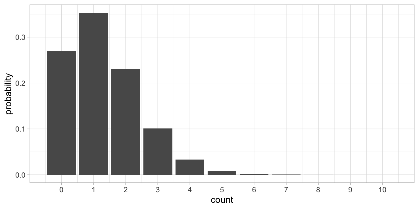
Figure 14.3: Poisson distribution with lambda = 1.31.
The last value of previous for which we calculate \(\lambda\) is +2,
representing a high-performing student. We then get
\(\lambda=\textrm{exp}(0.1576782 -0.0548685 \times 2)= 1.05\). A Poisson
distribution with \(\lambda=1.05\) is depicted in Figure
14.4.
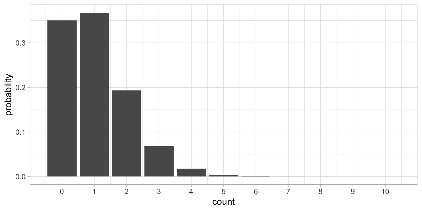
Figure 14.4: Poisson distribution with lambda = 1.05.
If we superimpose these three figures, we obtain Figure 14.5, where we see that the higher the average score on previous assignments, the lower the expected score on the present assignment.
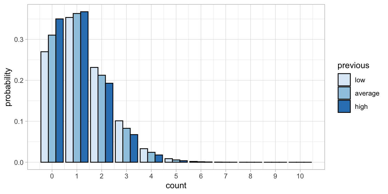
Figure 14.5: Three different Poisson distributions with lambdas 0.85, 1.31, and 1.05, for three different kinds of students.
We found that in this data set, previous high marks for assignments predicted a higher mark for the present assignment. In the next section we will see how to perform the analysis in R, and how to check whether there is also a relationship in the population of students.
14.2 Poisson regression in R
Poisson regression is a form of a generalised linear model analysis,
similar to logistic regression. However, instead of using a Bernoulli
distribution we use a Poisson distribution. For a numeric predictor like
the variable previous, the syntax is as follows.
model <- data %>%
  glm(score ~ previous, family = poisson, data = .)
model %>% tidy()
## # A tibble: 2 x 5
## term estimate std.error statistic p.value
## <chr> <dbl> <dbl> <dbl> <dbl>
## 1 (Intercept) 0.158 0.0925 1.71 0.0881
## 2 previous -0.0549 0.0899 -0.610 0.542confint(model)## Waiting for profiling to be done...## 2.5 % 97.5 %
## (Intercept) -0.02919483 0.3335813
## previous -0.23069637 0.1215225We see the same values for the intercept and the effect of previous as
in the previous section. We now also see 95% confidence intervals for
these parameter values. For both, the value 0 is included in the
confidence intervals, therefore we know that we cannot reject the
null-hypotheses that these values are 0 in the population of students.
This is also reflected by the test statistics. Remember that the
\(z\)-statistic is computed by \(b/SE\). For large enough samples, the
\(z\)-statistic follows a standard normal distribution. From that
distribution we know that a value of -0.610 is not significant at the 5%
level. It has an associated \(p\)-value of 0.542.
We can write:
"Scores for the assignment (1-4) for 100 students were analysed using a generalised linear model with a Poisson distribution (Poisson regression), with independent variable previous. The scores were not predicted by the average score of previous assignments, \(b = -0.06, z = -0.61, p = .54\). Therefore we found no evidence of a relationship between the average of previous assignments and the score on the present assignment in the population of students."
Suppose we also have a categorical predictor, for example the degree
that the students are working for. Some do the assignment for a
bachelor’s degree (degree = "Bachelor"), some for a master’s degree
(degree= "Master"), and some for a PhD degree (degree = "PhD"). The
code would then look like:
model2 <- data %>%
glm(score ~ degree, family = poisson, data = .)
model2 %>%
  tidy()
## # A tibble: 3 x 5
## term estimate std.error statistic p.value
## <chr> <dbl> <dbl> <dbl> <dbl>
## 1 (Intercept) -0.231 0.192 -1.20 0.231
## 2 degreeMaster 0.495 0.246 2.02 0.0437
## 3 degreePhD 0.584 0.241 2.42 0.0156confint(model2)## Waiting for profiling to be done...## 2.5 % 97.5 %
## (Intercept) -0.63302394 0.1243547
## degreeMaster 0.02046594 0.9877380
## degreePhD 0.11875363 1.0698921Note that only the independent variable has changed.
We see that the degree = "Bachelor" category is used as the reference
category. If we make a prediction for the group of students that is
studying for a PhD degree, we have
\(\lambda = \textrm{exp}(-0.231 + 0.584) = \textrm{exp}(0.353)=1.4\). For
the students studying for a Master’s degree we have
\(\lambda = \textrm{exp}(-0.231 + 0.495) =1.3\) and for students studying
for their Bachelor’s degree we have
\(\lambda = \textrm{exp}(-0.231) =0.8\). These \(\lambda\)-values correspond
to the expected count in a Poisson distribution, so for Bachelor
students we expect a score of \(0.8\), for Master students we expect a
score of \(1.3\) and for Phd students a score of \(1.4\). Are these
differences in scores also present in the population? We see that the
effect for degree = "Master" is significant, \(z=2.02, p=0.04\), so
there is a difference in score between students studying for a
Bachelor’s degree and students studying for a Master’s. The effect for
degree = PhD is also significant, \(z=0.584, p=0.016\), so there is a
difference in assignment scores between Bachelor students and PhD
students.
Remember that for the linear model, when we wanted to compare more than
two groups at the same time, we used an \(F\)-test to test for an overall
difference in group means. Also for the generalised linear model, we
might be interested in whether there is an overall difference in scores
between Bachelor, Master and PhD students. For that we need to perform
an analysis of variance.
model2 %>%
  anova(test = "Chisq")
## Analysis of Deviance Table
##
## Model: poisson, link: log
##
## Response: score
##
## Terms added sequentially (first to last)
##
##
## Df Deviance Resid. Df Resid. Dev Pr(>Chi)
## NULL 99 228.44
## degree 2 6.8186 97 221.62 0.03306 *
## ---
## Signif. codes: 0 '***' 0.001 '**' 0.01 '*' 0.05 '.' 0.1 ' ' 1However, what we see here is not an analysis of variance, but a model
comparison (an Analysis of Deviance Table is plotted). A model with the
predictor degree is compared to a baseline model with only an
intercept, the so-called null model. The model with only an intercept
has 99 residual degrees of freedom. The model with an intercept and the
effect of degree has only 97 residual degrees of freedom. The
difference of 2 degrees of freedom comes from the fact that the model
with degree requires estimating the effects of two dummy variables.
For both models the deviance is calculated. This deviance is based on
the method that is used for estimating the parameters. Where in linear
models, usually OLS is used (least squares principle), in generalised
methods usually the method of Maximum Likelihood is used. The difference
in the likelihoods of the two models says something about how
significant the effect of the predictor, in this case degree, is. It
so happens that minus twice the difference in the logarithm of the
likelihood has a distribution close to the chi-square distribution.
Minus twice the log-likelihood of a model is called the deviance. The
difference between two deviances is also called a deviance. Here we see
a deviance of 6.8186 for the difference between the two models. When we
look up what the proportion of the chi-square distribution with 2
degrees of freedom is larger than 6.8186, we know the \(p\)-value. This is
exactly what R does, and the output shows a \(p\)-value of 0.03306. This
\(p\)-value tells us whether the null-hypothesis that the expected scores
in the three groups of students are the same can be rejected. We report:
"The null-hypothesis that the expected scores in the three groups were equal was tested with a Poisson regression with degree as the independent variable. Results showed that the null-hypothesis could be rejected, \(\chi^2(2) = 6.82, p = .03\)."
14.3 Interaction effects in Poisson models
In the previous section we looked at a count variable, the number of criteria fulfilled, and we wanted to predict it from the degree that students were studying for. Let’s look at an example where we want to predict a count variable using two categorical predictors.
In 1912, the ship Titanic sank after the collision with an iceberg. There were 2201 people on board that ship. Some of these were male, others were female. Some were passengers, others were crew, and some survived, and some did not. For the passengers there were three groups: those travelling first class, second class and third class. There were also children on board. If we focus on only the adults, suppose we want to know whether there is a relationship between the sex and the counts of people that survived the disaster. Table 14.2 gives the counts of survivors for males and females separately.
| count | |
|---|---|
| Male | 338 |
| Female | 316 |
Let’s analyse this data set with R. First we load the Titanic dataset
and restructure the data to get counts for the numbers of females and
males.
data("Titanic")
# count the totals of females and males that survived
data <- as.matrix(apply(Titanic, c(2, 3, 4), sum)[ , 2, 2])
# give the variable the name 'count'
colnames(data) = "count"
# there are two cases and only 1 variable
dim(data)
## [1] 2 1# sex labels are only row labels. Introduce a variable sex
data <- data.frame(sex = c("Male", "Female"), data)
dim(data)## [1] 2 2data## sex count
## Male Male 338
## Female Female 316Next, our dependent variable is count, and the independent variable is
sex. Let’s do a Poisson regression.
model <- data %>%
  glm(count ~ sex, family = poisson, data = .)
model %>% tidy()
## # A tibble: 2 x 5
## term estimate std.error statistic p.value
## <chr> <dbl> <dbl> <dbl> <dbl>
## 1 (Intercept) 5.76 0.0563 102. 0
## 2 sexMale 0.0673 0.0783 0.860 0.390From the output we see that the expected count for females (the reference group) is \(\textrm{exp}(5.76)=317.3\) and the expected count for males is \(\textrm{exp}(5.76 + 0.0673)=339.4\). These expected counts are close to the observed counts of males and females. The only reason that they differ from the observed is because of rounding errors. From the \(z\)-statistic, we see that the difference in counts between males and females is not significant, \(z=0.86, p=.39\)29.
The difference in these counts is very small. But does this tell us that women were as likely to survive as men? Note that we have only looked at those who survived. How about the people that perished: were there more men that died than women? Table 14.3 shows the counts of male survivors, female survivors, male non-survivors and female non-survivors. Then we see a different story: on the whole there were many more men than women, and a relatively small proportion of the men survived. Of the men, most of them perished: 1329 perished and only 338 survived, a survival rate of 20.3%. Of the women, most of them survived: 109 perished and 316 survived, yielding a survival rate of 74%. Does this tell us that women are much more likely than men to survive collisions with icebergs?
| sex | survived | count |
|---|---|---|
| Male | 0 | 1329 |
| Female | 0 | 109 |
| Male | 1 | 338 |
| Female | 1 | 316 |
Let’s first run a multiple Poisson regression analysis including the
effects of both sex and survival. We first need to restructure the data
a bit, so that we have both variables sex and survived.
data <- as.matrix(apply(Titanic, c(2, 3,4), sum)[ , 2, ])
data <- as.vector(data)
data <- matrix(data, 4, 1)
sex <- rep(c("Male", "Female"), 2)
survived <- rep(c(0, 1), each = 2)
data <- data.frame(sex, survived, count = data)
data
## sex survived count
## 1 Male 0 1329
## 2 Female 0 109
## 3 Male 1 338
## 4 Female 1 316Next, we run the multiple Poissson regression.
model2 <- data %>%
  glm(count ~ sex + survived, family = poisson, data = .)
model2 %>% tidy()
## # A tibble: 3 x 5
## term estimate std.error statistic p.value
## <chr> <dbl> <dbl> <dbl> <dbl>
## 1 (Intercept) 5.68 0.0507 112. 0
## 2 sexMale 1.37 0.0543 25.2 1.38e-139
## 3 survived -0.788 0.0472 -16.7 1.20e- 62where sex is treated as a factor, since it is a string variable, and
survival as a numeric variable (since survived is coded as a dummy).
From the parameter values in the output, we can calculate the predicted
numbers of male (sex = Male) and female (sex = Female) that survived
and perished. The reference group consists of individuals that perished
(survived = 0) and are female. For perished females we have
\(\textrm{exp}(5.68)=292.95\), for female survivors we have
\(\textrm{exp}(5.68 - 0.788)=133.22\), for male survivors we have
\(\textrm{exp}(5.68 + 1.37 - 0.788)=524.27\) and for male non-survivors we
have \(\textrm{exp}(5.68 + 1.37)=1152.86\).
These predicted numbers are displayed in Figure
14.6. It
also shows the observed counts. The pattern that is observed is clearly
different from the one that is predicted from the generalised linear
model. The linear model predicts that there are fewer survivors than
non-survivors, irrespective of sex, but we observe that in females,
there are more survivors than non-survivors. It seems that sex is a
moderator of the effect of survival on counts.
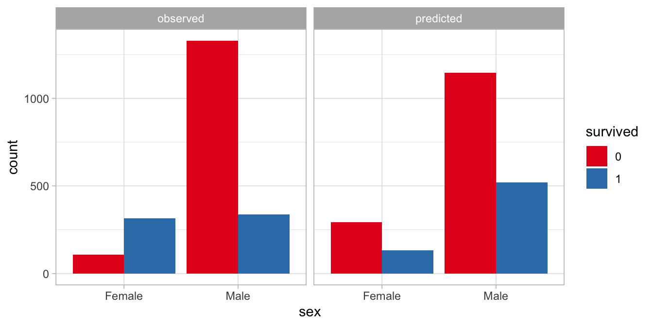
Figure 14.6: Difference between observed and predicted numbers of passengers.
In order to test this moderation effect, we run a new generalised linear
model for counts including an interaction effect of sex by survived.
This is done in R by adding sex:survived:
model3 <- data %>%
glm(count ~ sex + survived + sex:survived, family = poisson, data = .)
model3 %>% tidy()## # A tibble: 4 x 5
## term estimate std.error statistic p.value
## <chr> <dbl> <dbl> <dbl> <dbl>
## 1 (Intercept) 4.69 0.0958 49.0 0
## 2 sexMale 2.50 0.0996 25.1 4.92e-139
## 3 survived1 1.06 0.111 9.58 9.50e- 22
## 4 sexMale:survived1 -2.43 0.127 -19.2 3.12e- 82When we plot the predicted counts from this new model with an interaction effect, we see that they are exactly equal to the counts that are actually observed in the data, see Figure 14.7.
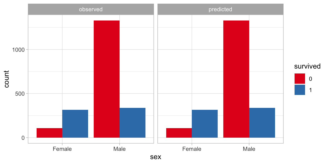
Figure 14.7: Difference between observed and predicted numbers of passengers. Predictions based on a model with an interaction effect.
From the output we see that the interaction effect is significant, \(z=-19.2, p < .001\). If we regard this data set as a random sample of all ships that sink after collision with an iceberg, we may conclude that in such situations, sex is a significant moderator of the difference in the numbers of survivors and non-survivors. One could also say: the proportion of people that survive a disaster like this is different in females than it is in males.
14.4 Cross-tabulation and the Pearson chi-square statistic
The data on male and female survivors and non-survivors are often tabulated in a cross-table like in Table 14.4
| No | Yes | |
|---|---|---|
| Male | 1329 | 338 |
| Female | 109 | 316 |
In the previous section these counts were analysed using a generalised linear model with a Poisson distribution and an exponential link function. We wanted to know whether there was a significant difference in the proportion of survivors for men and women. In this section we discuss an alternative method of analysing count data. We describe an alternative statistic for the moderation effect of one variable of the effect of another variable: the Pearson chi-square.
First, let’s have a look at the overall survival rate. In total there were 654 people that survived and 1438 people that did not survive. Table 14.5 shows these column totals.
| No | Yes | |
|---|---|---|
| Male | 1329 | 338 |
| Female | 109 | 316 |
| Total | 1438 | 654 |
Looking at these total numbers of survivors and non-survivors, we can calculate the proportion of survivors overall (the survival rate) as \(654/(654+1438)= 0.31\). Table 14.6 shows the totals for men and women, as well as the overall total number of adults.
| No | Yes | Total | |
|---|---|---|---|
| Male | 1329 | 338 | 1667 |
| Female | 109 | 316 | 425 |
| Total | 1438 | 654 | 2092 |
Suppose we only know that of the 2092 people, 1667 were men, and of all people, 654 survived. Then suppose we pick a random person from these 2092 people. What is the probability that we get a male person that survived, given that sex and survival have nothing to do with each other?
Well, from probability theory we know that if two events \(A\) and \(B\) are independent (unrelated), the probability of observing \(A\) and \(B\) at the same time, is equal to the product of the probability of event \(A\) and the probability of event \(B\).
\[Prob(A \& B) = Prob(A) \times Prob(B)\]
If sex and survival are independent from each other, then the probability of observing a male survivor is equal to the probability of seeing a male times the probability of seeing a survivor. The probability for survival is 0.31, as we saw earlier, and the probability of seeing a male is equal to the proportion of males in the data, which is \(1667/2092 =0.8\). Therefore, the probability of seeing a male survivor is \(0.8 \times 0.31 =0.24\). The expected number of male survivors is then that probability times the total number of people, \(0.24 \times 2092= 502.08\). Similarly we can calculate the expected number of non-surviving males, the number of surviving females, and the number of non-surviving females.
These numbers, after rounding, are displayed in Table 14.7.
| No | Yes | |
|---|---|---|
| Male | 1155 | 519 |
| Female | 289 | 130 |
The expected numbers in Table 14.7 are quite different from the observed numbers in Table 14.4. Are the differences large enough to think that the two events of being male and being a survivor are NOT independent? If the expected numbers on the assumption of independence are different enough from the observed numbers, then we can reject the null-hypothesis that being male and being a survivor have nothing to do with each other. To measure the difference between expected and observed counts, we need a test statistic. Here we use Pearson’s chi-square statistic. It involves calculating the difference between the observed and expected numbers in the respective cells, and standardise them by the expected number. Here’s how it works:
For each cell, we take the predicted count and subtract it from the observed count. For instance, for the male survivors, we expected 519 but observed 338. The difference is therefore \(338-519= -181\). Then we take the square of this difference, \(181^2=32761\). Then we divide this number by the expected number, and then we get \(32761/519=63.1233141\). We do exactly the same thing for the male non-survivors, the female survivors and the female non-survivors. Then we add these 4 numbers, and then we have the Pearson chi-square statistic. In formula form:
\[X^2 = \Sigma_i \frac{(O_i-E_i)^2}{E_i}\]
So for male survivors we get
\[\frac{(338-519)^2}{519} =63.1233141\]
For male non-survivors we get
\[\frac{(1329-1155)^2}{1155} =26.212987\]
For female survivors we get
\[\frac{(316-130)^2}{130} =266.1230769\]
and for female non-survivors we get
\[\frac{(109-289)^2}{289} =112.1107266\]
If we add these 4 numbers we have the chi-square statistic: \(X^2= 467.57\). Note that we only use the rounded expected numbers. Better would be to use the non-rounded numbers. Had we used the non-rounded expected numbers, we would have gotten \(X^2 = 460.87\).
Remember that in the Poissson regression earlier, the \(z\)-statistic for the sex by survived interaction effect was -19.2088233, see the earlier output. It tests exactly the same null-hypothesis as the Pearson chi-square: that of independence, or in other words, that the numbers can be explained by only two main effects, sex and survival.
If the data set is large enough and the numbers are not too close to 0, the same conclusions will be drawn, whether from a \(z\)-statistic for an interaction effect in a Poisson regression model, or from a cross-tabulation and computing a Pearson chi-square. The advantage of the Poisson regression approach is that you can do much more with them, for instance more than two predictors, and that you make it more explicit that when computing the statistic, you take into account the main effects of the variables. You do that also for the Pearson chi-square, but it is less obvious: we did that by first calculating the probability of survival and second calculating the proportion of males.
We can report the results from the cross-tabulation as follows:
"We tested the null-hypothesis that the variables sex and survival are not related with a Pearson chi-square test. The results showed that the null-hypothesis could be rejected, \(\chi^2(1) = 460.87, p < .001\)."
The degrees of freedom for Pearson’s chi-square are determined by the number of categories for variable 1, \(K_1\), and the number of categories for variable 2, \(K_2\): \(\textrm{df} = (K_1 - 1)(K_2 - 1)\). The \(p\)-value can be found by looking up how much of the chi-square distribution with 1 degree of freedom is more than 460.87:
pchisq(460.87, df = 1, lower.tail = F)## [1] 0.00000000000000000000000000000000000000000000000000000000000000000000000000000000000000000000000000000310859814.5 Poisson regression or logistic regression?
In the previous section we analysed the relationship between the
variable sex of the person on board the Titanic, and the variable
survived: whether or not a person survived the shipwreck. We found a
relationship between these two variables by studying the
cross-tabulation of the counts, and testing that relationship using a
Pearson chi-square statistic. In the section before that, we saw that
this relationship could also be tested by applying a Poisson regression
model and looking at the sex by survived interaction effect. These
methods are equivalent.
There is yet a third way to analyse the sex and survived variables.
Remember that in the previous chapter we discussed logistic regression.
In logistic regression, a dichotomous variable (a variable with only two
values, say 0 and 1) is the dependent variable, with one or more numeric
or categorical independent variables. Both sex and survived are
dichotomous variables: male and female, and survived yes or survived no.
In principle therefore, we could do a logistic regression: for example
predicting whether a person is a male or female, on the basis of whether
they survived or not, or the other way around, predicting whether people
survive or not, on the basis of whether a person is a woman or a man.
What variable is used here as your dependent variable, depends on your research question. If your question is whether females are more likely to survive than men, perhaps because of their body fat composition, or perhaps because of male chivalry, then the most logical choice is to take survival as the dependent variable and sex as the independent variable.
The code for a logistic regression then looks like
model <- data %>%
glm(survived ~ sex, family = binomial, data = .)Note however that the data can be in the wrong format. For the Poisson regression, the data were in the form of what we see in Table 14.3. However, for a logistic regression, we need the data in long format, like in Table @(tab:gen28). For every person on-board the ship, we have to know their sex and their survival status.
| ID | sex | survived |
|---|---|---|
| 1030 | Male | 0 |
| 1289 | Male | 0 |
| 1685 | Male | 1 |
| 1736 | Male | 1 |
| 1998 | Female | 1 |
## # A tibble: 2 x 5
## term estimate std.error statistic p.value
## <chr> <dbl> <dbl> <dbl> <dbl>
## 1 (Intercept) 1.06 0.111 9.58 9.50e-22
## 2 sexMale -2.43 0.127 -19.2 3.12e-82When we run the logistic regression, we see in the output that sex is a significant predictor of the survival status, \(b = -2.43, z = -19.2, p<.001\). The logodds for a male surviving the shipwreck is \(1.06 - 2.43 = -1.37\), and the logodds ratio for a female surviving the shipwreck is \(1.06\). These logodds correspond to probabilities of \(0.20\) and \(0.74\), respectively. Thus, women were much more likely to survive than men.
However, suppose you are the relative of a passenger on board a ship that shipwrecks. After two days, there is news that a person was found. The only thing known about the person is that he or she is alive. Your relative is your niece, so you’d like to know on the basis of the information that the person that was found is alive, what is the probability that that person is a woman, because then it could be your beloved niece! You could therefore run a logistic regression on the Titanic data to see to what extent the survival of a person predicts the sex of that person. First we have to turn the dependent variable into a dummy variable. Since we would be happy if a survivor is a female, we code Female as 1 and Male as 0. Next, we do the logistic regression where we switch the dependent and independent variables.
## # A tibble: 3 x 5
##   term        estimate std.error statistic   p.value
##   <chr>          <dbl>     <dbl>     <dbl>     <dbl>
## 1 (Intercept)    5.68     0.0507     112.  0
## 2 sexMale        1.37     0.0543      25.2 1.38e-139
## 3 survived -0.788 0.0472 -16.7 1.20e- 62From this output we conclude that survival is a significant predictor of
sex, \(b=2.43, z=19.2, p<.001\). The logodds ratio for a surviving person
to be a woman is \(-2.50 + 2.43= -0.07\), and the logodds ratio for a
non-surviving person to be a woman is \(-2.50\). These logodds ratios
correspond to probabilities of \(0.48\) and \(0.08\), respectively. Thus, if
you know that there is a person that survived the Titanic, it is about a
50-50% chance that it is a woman. If you think this is
counter-intuitive, remember that even though a large proportion of the
women survived the Titanic, there were many more men on-board than
women.
In summary, if you have count data, and both of the variables are
dichotomous, you have the choice whether to use a Poisson regression
model for counts or a logistic regression with one of the dichotomous
variables as dependent variables. The choice depends on the research
question: if your question involves prediction of a dichotomous
variable, logistic regression is the logical choice. If you have a
theory that one or more independent variables explain one other
variable, logistic regression is the logical choice. If however your
theory does not involve a natural direction or prediction of one
variable, and you are simply interested in associations among variables,
then Poisson regression of counts is the obvious choice.
Note that a hypothesis test is a bit odd here: there is no clear population that we want to generalise the results to: there was only one Titanic disaster. Also, here we have data on the entire population of those people on board the Titanic, there is no random sample here.↩︎