Chapter 6 Categorical predictor variables
6.1 Dummy coding
library(tidyverse)
library(broom)
library(knitr)
library(latex2exp)
As we have seen in Chapter 1, there are largely two different types of variables: numeric variables and categorical variables. Numeric variables say something about how much of an attribute is in an object: for instance height (measured in inches) or heat (measured in degrees Celsius). Categorical variables say something about the quality of an attribute: for instance colour (red, green, yellow) or type of seating (aisle seat, window seat). We have also seen a third type of variable: ordinal variables. Ordinal variables are somewhat in the middle between numeric variables and categorical variables: they are about quantitative differences between objects (e.g., size) but the values are sharp disjoint categories (small, medium, large), and the values are not expressed using units of measurements.
In the chapters on simple and multiple regression we saw that both the dependent and the independent variables were all numeric. The linear model used in regression analysis always involves a numeric dependent variable. However, in such analyses it is possible to use categorical independent variables. In this chapter we explain how to do that and how to interpret the results.
The basic trick that we need is dummy coding. Dummy coding involves making one or more new variables, that reflects the categorisation seen with a categorical variable. First we focus on categorical variables with only two categories (dichotomous variables). Later in this chapter, we will explain what to do with categorical variables with more than two categories (nominal variables).
Imagine we study bus companies and there are two different types of
seating in buses: aisle seats and window seats. Suppose we ask 5 people,
who have travelled from Amsterdam to Paris by bus during the last 12
months, whether they had an aisle seat or a window seat during their
last trip, and how much they paid for the trip. Suppose we have the
variables person, seat and price. Table
6.1 shows
the anonymised data. There we see the dichotomous variable seat with
values ‘aisle’ and ‘window.’
| person | seat | price |
|---|---|---|
| 001 | aisle | 57 |
| 002 | aisle | 59 |
| 003 | window | 68 |
| 004 | window | 60 |
| 005 | aisle | 61 |
With dummy coding, we make a new variable that only has values 0 and 1,
that conveys the same information as the seat variable. The resulting
variable is called a dummy variable. Let’s call this dummy variable
window and give it the value 1 for all persons that travelled in a
window seat. We give the value 0 for all persons that travelled in an
aisle seat. We can also call the new variable window a boolean
variable with TRUE and FALSE, since in computer science, TRUE is coded
by a 1 and FALSE by a 0. Another name that is sometimes used is an
indicator variable. Whatever you want to call it, the data matrix
including the new variable is displayed in Table
6.2.
| person | seat | window | price |
|---|---|---|---|
| 001 | aisle | 0 | 57 |
| 002 | aisle | 0 | 59 |
| 003 | window | 1 | 68 |
| 004 | window | 1 | 60 |
| 005 | aisle | 0 | 61 |
What we have done now is coding the old categorical variable seat into
a variable window with values 0 and 1 that looks numeric. Let’s see
what happens if we use a linear model for the variables price
(dependent variable) and window (independent variable). The linear
model is:
\[\begin{aligned} \texttt{price} &= b_0 + b_1 \texttt{window} + e \nonumber\\ e &\sim N(0,\sigma^2_e)\nonumber \end{aligned}\]
Let’s use the bus trip data and determine the least squares regression line. We find the following linear equation:
\[\widehat{\texttt{price}} = 59 + 5 \times \texttt{window}\]
If the variable window has the value 1, then the expected or predicted
price of the bus ticket is, according to this equation,
\(59 + 5\times 1= 64\). What does this mean? Well, all persons who had a
window seat also had a value of 1 for the window variable. Therefore
the expected price of a window seat equals 64. By the same token, the
expected price of an aisle seat (window = 0) is \(59 + 5\times 0= 59\),
since all those with an aisle seat scored 0 on the window variable.
You see that by coding a categorical variable into a numeric dummy
variable, we can describe the ‘linear’ relationship between the type of
seat and the price of the ticket. Figure
6.1 shows
the relationship between the numeric variable window and the numeric
variable price.
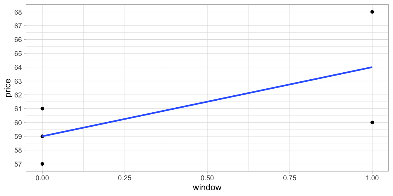
Figure 6.1: Relationship between dummy variable window and price.
Note that the blue regression line goes straight through the mean of the
prices for window seats (window = 1) and the mean of the prices for
aisle seats (window = 0). In other words, the linear model with the
dummy variable actually models the group means of people with window
seats and people with aisle seats.
Figure 6.2
shows the same regression line but now for the original variable seat.
Although the analysis was based on the dummy variable window, it is
more readable for others to show the original categorical variable
seat.
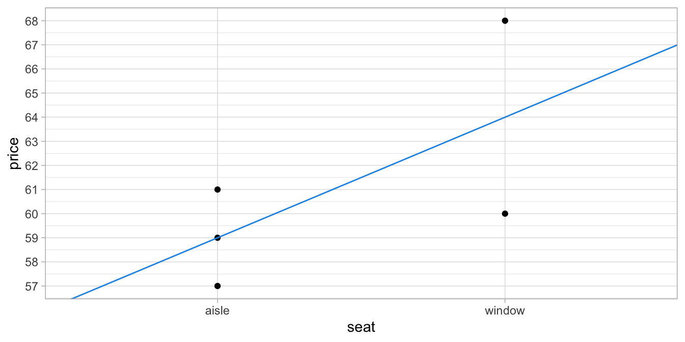
Figure 6.2: Relationship between type of seat and price.
6.2 Using regression to describe group means
In the previous section we saw that if we replace a categorical variable with a numeric dummy variable with values 0 and 1, we can use a linear model to describe the relationship between a categorical independent variable and a numeric dependent variable. We also saw that if we take the least squares regression line, this line goes straight through the averages, the group means. The line goes straight through the group means because then the sum of the squared residuals is at its smallest value (the least squares principle). Have a look at the bus trip data again in Figure 6.1 and see if you can derive the residuals and the squared residuals. These are displayed in Table 6.3.
| person | seat | window | price | e | e_squared |
|---|---|---|---|---|---|
| 001 | aisle | 0 | 57 | -2 | 4 |
| 002 | aisle | 0 | 59 | 0 | 0 |
| 003 | window | 1 | 68 | 4 | 16 |
| 004 | window | 1 | 60 | -4 | 16 |
| 005 | aisle | 0 | 61 | 2 | 4 |
If we take the sum of the squared residuals we obtain 40. Now if we use a slightly different slope, so that we no longer go straight through the average prices for aisle and window seats (see Figure 6.3) and we compute the predicted values, the residuals and the squared residuals (see Table 6.4), we obtain a higher sum: 40.05.
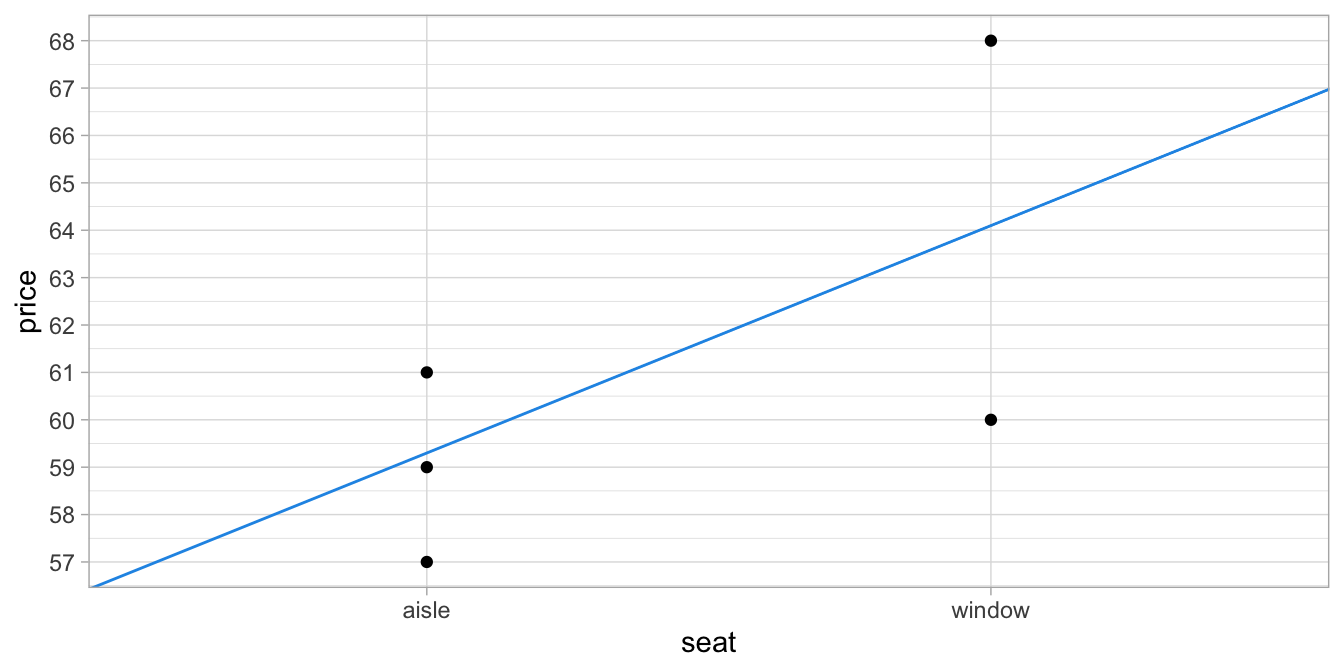
Figure 6.3: Relation between type of seat and price, with the regression line being not quite the least squares line.
| person | seat | window | price | wrongpredict | e | e_squared |
|---|---|---|---|---|---|---|
| 001 | aisle | 0 | 57 | 59.1 | -2.1 | 4.41 |
| 002 | aisle | 0 | 59 | 59.1 | -0.1 | 0.01 |
| 003 | window | 1 | 68 | 63.9 | 4.1 | 16.81 |
| 004 | window | 1 | 60 | 63.9 | -3.9 | 15.21 |
| 005 | aisle | 0 | 61 | 59.1 | 1.9 | 3.61 |
Only the least squares regression line goes through the observed average prices of aisle seats and window seats. Thus, we can use the least squares regression equation to describe observed group means for categorical variables.
Conversely, when you know the group means, it is very easy to draw the regression line: the intercept is then the mean for the category coded as 0, and the slope is equal to the mean of the category coded as 1 minus the mean of the category coded as 0 (i.e., the intercept). Check Figure 6.1 to verify this yourself. But we can also show this for a new data set.
We look at results from an experiment to compare yields (as measured by dried weight of plants) obtained under a control and two different treatment conditions. Let’s plot the data first, where we only compare the two experimental conditions (see Figure 6.4).
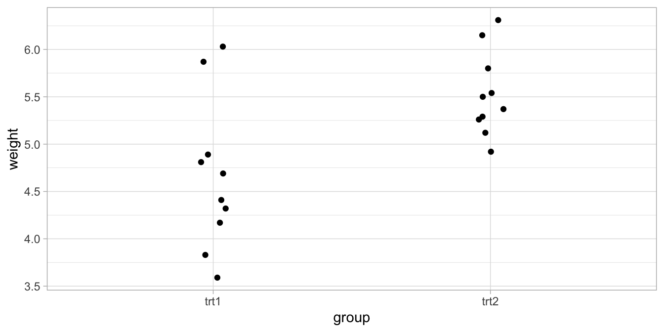
Figure 6.4: Data on yield under two experimental conditions: treatment 1 and treatment 2.
With treatment 1, the average yield turns out to be 4.661, and with
treatment 2, the average yield is 5.526. Suppose we make a new dummy
variable treatment2 that is 0 for treatment 1, and 1 for treatment 2.
Then we have the linear equation:
\[\widehat{\texttt{weight}} = b_0 + b_1 \times \texttt{treatment2}\]
If we fill in the dummy variable and the expected weights (the means!), then we have the linear equations:
\[\begin{aligned} 4.661 &= b_0 + b_1 \times 0 = b_0 \nonumber\\ 5.526 &= b_0 + b_1 \times 1 = b_0 + b_1 \nonumber \end{aligned}\]
So from this, we know that intercept \(b_0 = 4.661\), and if we fill that in for the second equation above, we get the slope:
\[b_1 = 5.526-b_0= 5.526 -4.661= 0.865.\]
Thus, we get the linear equation
\[ \begin{equation} \widehat{\texttt{weight}} = 4.661 + 0.865\times \texttt{treatment} \tag{6.1} \end{equation} \]
Since this regression line goes straight through the average yield for each treatment, we know that this is the least squares regression equation. We could have obtained the exact same result with a regression analysis using statistical software. But this was not necessary: because we knew the group means, we could find the intercept and the slope ourselves by doing the math.
The interesting thing about a dummy variable is that the slope of the regression line is exactly equal to the differences between the two averages. If we look at Equation (6.1), we see that the slope coefficient is 0.865 and this is exactly equal to the difference in mean weight for treatment 1 and treatment 2. Thus, the slope coefficient for a dummy variable indicates how much the average of the treatment that is coded as 1 differs from the treatment that is coded as 0. Here the slope is positive so that we know that the treatment coded as 1 (trt2), leads to a higher average yield than the treatment coded as 0 (trt1). This makes it possible to draw inferences about differences in group means.
6.3 Making inferences about differences in group means
In the previous section we saw that the slope in a dummy regression is equal to the difference in group means. Suppose researchers are interested in the effects of different treatments on yield. They’d like to know what the difference is in yield between treatments 1 and 2, using a limited sample of 20 data points. Based on this sample, they’d like to generalise to the population of all yields based on treatments 1 and 2. They adopt a type I error rate of \(\alpha=0.05\).
The researchers analyse the data and they find the regression table as
displayed in Table 6.5. The 95% confidence interval for the slope is
from 0.26 to 1.47. This means that reasonable values for the
population difference between the two treatments on yield lie within
this interval. All these values are positive, so we reasonably believe
that treatment 2 leads to a higher yield than treatment 1. We know that
it is treatment 2 that leads to a higher yield, because the slope in the
regression equation refers to a variable grouptrt2 (see Table
6.5).
| term | estimate | std.error | statistic | p.value | conf.low | conf.high |
|---|---|---|---|---|---|---|
| (Intercept) | 4.661 | 0.2031985 | 22.938167 | 0.0000000 | 4.2340959 | 5.087904 |
| grouptrt2 | 0.865 | 0.2873660 | 3.010098 | 0.0075184 | 0.2612664 | 1.468734 |
Thus, a dummy variable has been created, grouptrt2, where trt2 has
been coded as 1 (and trt1 consequently coded as 0). In the next section,
we will see how to do this yourself.
If the researchers had been interested in testing a null-hypothesis about the differences in mean yield between treatment 1 and 2, they could also use the 95% confidence interval for the slope. As it does not contain 0, we can reject the null-hypothesis that there is no difference in group means at an \(\alpha\) of 5%. The exact \(p\)-value can be read from Table 6.5 and is equal to 0.01.
Thus, based on this regression analysis the researchers can write in a report:
"There is a significant difference between the yield after treatment 1 and the yield after treatment 2, \(t(18) = 3.01, p=0.01\). Treatment 2 leads to a yield of about 0.87 (SE = 0.29) more than treatment 1 (95% CI: 0.26, 1.47)."
6.4 Regression analysis using a dummy variable in R
When your independent variable is a categorical variable, the code that you use in R is the same as with a numeric independent variable. For instance, if you want to predict yield from the treatment group, you could run the following R code:
data("Plantgrowth")
PlantGrowth %>%
  filter(group != "ctrl") %>%
  lm(weight ~ group, .) %>%
  tidy()
In this code, we take the PlantGrowth data frame that is available in
R, we omit the data points from the control group (because we are only
interested in the two treatment groups), and we model weight as a
function of group. What then happens depends on the data type of
group. Let’s take a quick look at the variables:
PlantGrowth %>%
  select(weight, group) %>%
  str()
## 'data.frame': 30 obs. of 2 variables:
## $ weight: num 4.17 5.58 5.18 6.11 4.5 4.61 5.17 4.53 5.33 5.14 ...
## $ group : Factor w/ 3 levels "ctrl","trt1",..: 1 1 1 1 1 1 1 1 1 1 ...We see that the dependent variable weight is of type numeric (num),
and that the independent variable group is of type factor. If the
independent variable is of type factor, R will automatically make a
dummy variable for the factor variable. This will not happen if the
independent variable is of type numeric.
So here group is a factor variable. Below we see the regression table
that results from the linear model analysis.
data("PlantGrowth")
out <- PlantGrowth %>%
  filter(group != "ctrl") %>%
  lm(weight ~ group, .)
out %>%
  tidy()
## # A tibble: 2 x 5
## term estimate std.error statistic p.value
## <chr> <dbl> <dbl> <dbl> <dbl>
## 1 (Intercept) 4.66 0.203 22.9 8.93e-15
## 2 grouptrt2 0.865 0.287 3.01 7.52e- 3We no longer see the group variable, but we see a new variable called
grouptrt2. Apparently, this new variable was created by R to deal with
the group variable being a factor variable. The slope value of 0.865
now refers to the effect of treatment 2, that is, treatment 1 is the
reference category and the value 0.865 is the added effect of treatment
2 on the yield. We should therefore interpret these results as that in
the sample data, the mean of the treatment 2 data points was 0.865
higher than the mean of the treatment 1 data points.
Here, R automatically picked the treatment 1 group as the reference
group. In case you want to have treatment 2 as the reference group, you
could make your own dummy variable. For instance, make your own dummy
variable grouptrt1 in the following way and check whether it is indeed
stored as numeric in R:
PlantGrowth <- PlantGrowth %>%
 mutate(grouptrt1 = ifelse(group == "trt1", 1, 0))

PlantGrowth %>%
  select(weight, group, grouptrt1) %>%
  str()
## 'data.frame': 30 obs. of 3 variables:
## $ weight : num 4.17 5.58 5.18 6.11 4.5 4.61 5.17 4.53 5.33 5.14 ...
## $ group : Factor w/ 3 levels "ctrl","trt1",..: 1 1 1 1 1 1 1 1 1 1 ...
## $ grouptrt1: num 0 0 0 0 0 0 0 0 0 0 ...Next, you can run a linear model with the grouptrt1 dummy variable
that you created yourself:
out <- PlantGrowth %>%
  filter(group != "ctrl") %>%
  lm(weight ~ grouptrt1, .)
out %>%
  tidy()
## # A tibble: 2 x 5
## term estimate std.error statistic p.value
## <chr> <dbl> <dbl> <dbl> <dbl>
## 1 (Intercept) 5.53 0.203 27.2 4.52e-16
## 2 grouptrt1 -0.865 0.287 -3.01 7.52e- 3The results now show the effect of treatment 1, with treatment 2 being the reference category. Of course the effect of -0.865 is now the opposite of the effect that we saw earlier (+0.865), when the reference category was treatment 2. The intercept has also changed, as the intercept is now the expected weight for the other treatment group. In other words, the reference group has now changed: the intercept is equal to the expected weight of the treatment 1 group.
In general, store variables that are essentially categorical as factor
variables in R. For instance, you could have a variable group that has
two values 1 and 2 and that is stored as numeric. It would make more
sense to first turn this variable into a factor variable, before using
this variable as a predictor in a linear model. You could turn the
variable into a factor only for the analysis and leaving the data frame
unchanged, like this:
model <- dataset %>%
lm(y ~ factor(group), data = .)
or change the data frame before the analysis
dataset <- dataset %>%
  mutate(group = factor(group))

model <- dataset %>%
lm(y ~ group, data = .)
R will always choose the category with the lowest internal integer value as the reference category. The internal values are chosen alphabetically. If that however makes the output hard to interpret, think of the best way to code your own dummy variable. For experimental designs, it makes sense to code control conditions as 0, and experimental conditions as 1 (you’re often interested in the effect of the experimental condition compared to the control condition, so the control condition is the reference group). For social surveys, if you want to compare how a social minority group scores relative to a social majority group, it makes sense to code the minority group as 1 and the social majority as 0. In educational studies, it makes sense to code an old teaching method as 0 and a new method as 1. In all of these cases, the slope can then be interpreted as the difference of the experimental procedure/new method/minority compared to the reference group, and the intercept can be interpreted as the mean of the reference group.
6.5 Two independent variables: one dummy and one numeric variable
In Chapter 4 we saw that we can have more than one predictor variable in a linear model. If we have two or more numeric variables, one usually talks about multiple regression models. When we have a categorical variable that we treat as a numeric dummy variable, then we can therefore also have linear models with both a categorical variable and a numeric variable.
Let’s return to the bus trip to Paris data. Suppose that one can choose the amount of leg room. There are seats with 60, 70 or 80 centimetres of leg room. You might expect that seats with more leg room are more expensive. To find out whether this is the case, you analyse the sample data from the 5 travellers. Leg room varies between 60 and 80 centimetres. Since you already know that the price of seats also depends on the type of seat (aisle or window), you analyse the data with the following linear model:
\[ \begin{eqnarray} \texttt{price} &=& b_0 + b_1 \texttt{window} + b_2 \texttt{legroom} + e \nonumber \\ e &\sim& N(0, \sigma^2) \nonumber \end{eqnarray} \]
That is, your independent variables are the dummy variable window (1
coding for window seat, 0 coding for aisle seat) and the numeric
variable legroom.
| term | estimate | std.error | statistic | p.value |
|---|---|---|---|---|
| (Intercept) | 41.50 | 9.71 | 4.27 | 0.05 |
| window | 5.00 | 2.50 | 2.00 | 0.18 |
| leg_room | 0.25 | 0.14 | 1.83 | 0.21 |
When we look at the output, we see the regression table in Table @ref(tab:legroom-table. When we fill in the coefficients, we obtain the following linear equation:
\[\widehat{\texttt{price}} = 41.5 + 5 \times \texttt{window} + 0.25 \times \texttt{legroom} \label{eq:two-predictors}\]
From Chapter 4 we know how to interpret the coefficients. The
slope coefficient for window should be interpreted as "the increase
in price if we change seat from aisle to window, given a certain amount
of legroom". That is, holding legroom constant, for instance at 60
centimetres, the difference between an aisle and a window seat equals 5
Euros. And of course, this difference is also 5 Euros when legroom
equals 70 centimetres, and also when legroom equals 80 centimetres.
Along the same vein, the slope coefficient for legroom should be
interpreted as "the increase in price for every unit increase in
legroom, given a certain type of seat". Thus, for an aisle seat, you
pay 0.25 Euros more for every extra centimetre. And this is also true
for window seats: every extra centimetre for your legs costs you 0.25
Euros.
The intercept of 41.5 means that the model predicts that you pay 41.5 if you happen to have 0 centimetres of leg room and an aisle seat (the reference category). Of course, a seat with 0 leg room does not exist, but it is simply what the model predicts, based on the data that are observed. The data and these predictions are visualised in Figure 6.5.
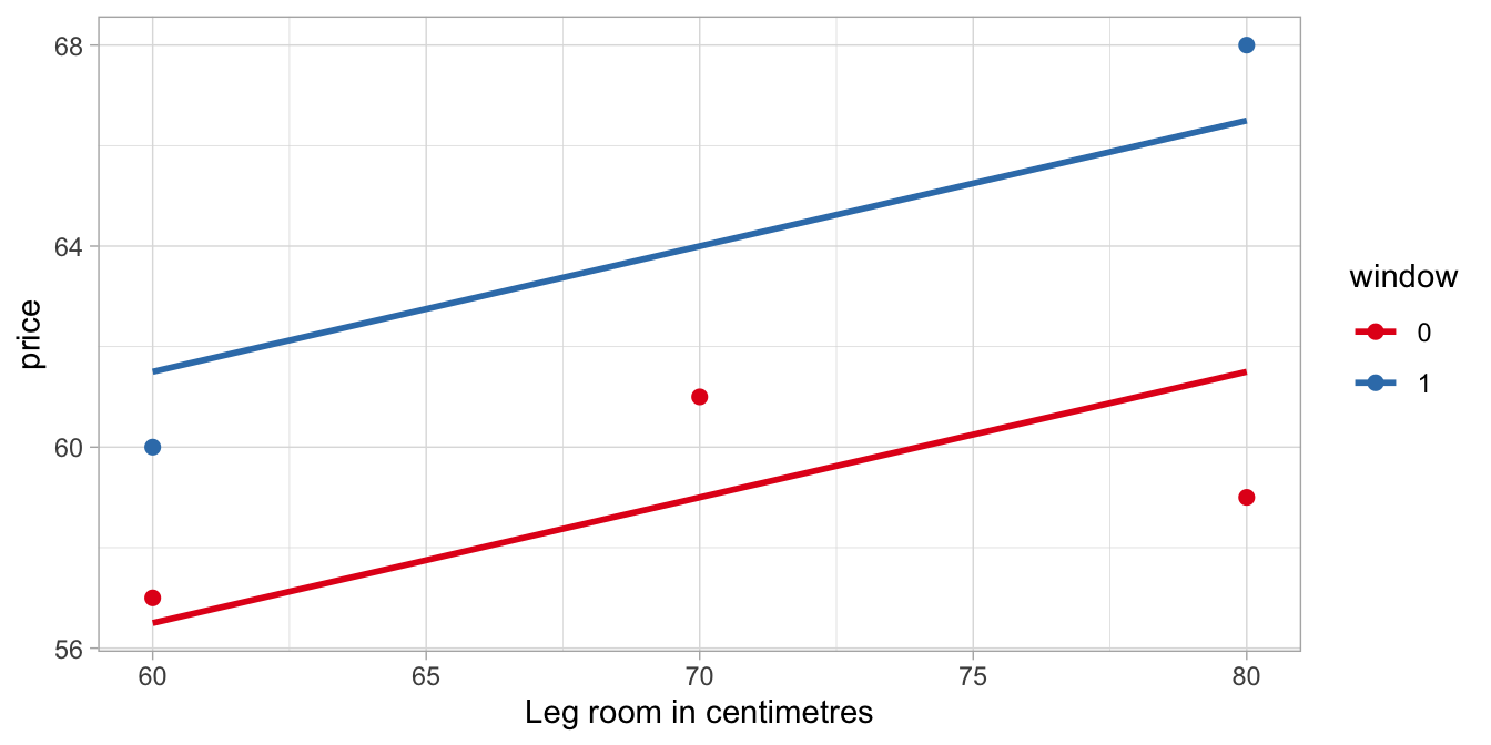
Figure 6.5: The bus trip to Paris data, with the predictions from a linear model with legroom and window as independent variables.
In order to visualise the relationship between the three variables
price, legroom and window, we plotted legroom on the horizontal
axis, and used different colours for the variable window. There are a
couple of things you should notice in this figure.
The first you should notice is that there are now two regression lines,
one for window seats and one for aisle seats. This is so because the
model makes different predictions for window and aisle seats. If we take
Equation
(??) and make predictions for aisle seats, we
fill in window = 0 and we get the following linear equation:
\[\widehat{\texttt{price}} = 41.5 + 5\times 0 + 0.25 \times \texttt{legroom} = 41.5 + 0.25 \times \texttt{legroom}\]
Thus, the regression line for aisle seats has an intercept of 41.5 and a
slope of 0.25. Now let’s fill in the equation for window seats, that is,
window = 1. Then we obtain
\[\widehat{\texttt{price}} = 41.5 + 5 \times 1 + 0.25 \times \texttt{legroom} = 46.5 + 0.25 \times \texttt{legroom}\]
That is, the regression line for window seats has an intercept that is
different: it is equal to the original intercept plus the slope of the
window variable, \(41.5 + 5 = 46.5\). On the other hand, the slope for
legroom is unchanged. With the same slope for legroom, the two
regression lines are therefore parallel.
The second you should notice from Figure 6.5 is that these two regression lines are not the least squares regression lines for window and aisle seats respectively. For instance, the regression line for window seats (the top one) should be steeper in order to minimise the difference between the data points and the regression line (the residuals). On the other hand, the regression line for aisle seats (the bottom one) should be less steep in order to have smaller residuals. Why is this so? Shouldn’t the regression lines minimise the residuals?
Yes they should! But there is a problem, because the model also implies, as we saw above, that the lines are parallel. Whatever we choose for values for the multiple regression equation, the regression lines for aisle and window seats will always be parallel. And under that constraint, the current parameter values give the lowest possible value for the sum of the squared residuals, that is, the the sum of the squared residuals for both regression lines taken together. The aisle seat regression line should be less steep, and the window seat regression line should be steeper to have a better fit with the data, but taken together, the estimated slope of 0.25 gives the lowest overall sum of squared residuals, given that the lines must be parallel.
It is possible though to have linear models where the lines are not parallel. This will be discussed in Chapter 10.
6.6 Dummy coding for more than two groups
In the previous sections we saw how to code a categorical variable with 2 categories (a dichotomous variable) into 1 dummy variable. In this section, we learn how to code a categorical variable with 3 categories into 2 dummy variables, and to code a categorical variable with 4 categories into 3 dummy variables, etcetera. That is, how to code nominal variables into sets of dummy variables.
Take for instance a variable Country, where in your data set, there
are three different values for this variable, for instance, Norway,
Sweden and Finland, or Zimbabwe, Congo and South-Africa. Let’s call
these countries A, B and C. Table
6.7 shows a data example where we see height
measurements on people from three different countries.
| ID | Country | height |
|---|---|---|
| 001 | A | 120 |
| 002 | A | 160 |
| 003 | B | 121 |
| 004 | B | 125 |
| 005 | C | 140 |
We can code this Country variable with three categories into two dummy
variables in the following way. First, we create a variable countryA.
This is a dummy variable, or indicator variable, that indicates whether
a person comes from country A or not. Those persons that do are coded 1,
and those that do not are coded 0. Next, we create a dummy variable
countryB that indicates whether or not a person comes from country B.
Again, persons that do are coded 1, and those that do not are coded 0.
The resulting variables are displayed in Table
6.8.
| ID | Country | height | countryA | countryB |
|---|---|---|---|---|
| 001 | A | 120 | 1 | 0 |
| 002 | A | 160 | 1 | 0 |
| 003 | B | 121 | 0 | 1 |
| 004 | B | 125 | 0 | 1 |
| 005 | C | 140 | 0 | 0 |
Note that we have now for every value of Country (A, B, or C) a unique
combination of the variables countryA and countryB. All persons from
country A have a 1 for countryA and a 0 for countryB; all those from
country B have a 0 for countryA and a 1 for countryB, and all those
from country C have a 0 for countryA and a 0 for countryB. Therefore
a third dummy variable countryC is not necessary (i.e., is redundant):
the two dummy variables give us all the country information we need.
Remember that with two categories, you only need one dummy variable, where one category gets 1s and another category gets 0s. In this way both categories are uniquely identified. Here with three categories we also have unique codes for every category. Similarly, if you have 4 categories, you can code this with 3 dummy variables. In general, when you have a variable with \(K\) categories, you can code them with \(K-1\) dummy variables.
6.7 Analysing categorical predictor variables in R
R contains a data set (PlantGrowth) on yield on a sample of thirty
observations (\(n=30\)), under three different conditions. We already saw
part of the data in Figure 6.4. The complete data consists of weight in three
different groups: treatment 1 (trt1), treatment 2 (trt2) and a
control group (ctrl). Now we want to model weight as a function of
the categorical variable group using a linear model. Again, we discuss
two options how to do that in R. First by creating your own dummy
variables, second by letting R create dummy variables automatically.
6.7.1 Creating your own dummy variables
Suppose you want to compare treatments 1 and 2 to your control
condition. Then it makes most sense to create two dummy variables, that
code for the treatment 1 group and the treatment 2 group, respectively.
Thus, we create a new variable treatment_1 and code every specimen
that belongs to treatment 1 as 1, and all other specimens as 0. Next, we
create a new variable treatment_2 and code every specimen that belongs
to treatment 2 as 1, and all other specimens as 0. The code is as
follows:
PlantGrowth <- PlantGrowth %>%
  mutate(treatment_1 = ifelse(group == "trt1", 1, 0),
         treatment_2 = ifelse(group == "trt2", 1, 0))
Next, we use these new dummy variables in a multiple regression analysis:
model1 <- PlantGrowth %>%
  lm(weight ~ treatment_1 + treatment_2, data = .)
model1 %>%
  tidy()
## # A tibble: 3 x 5
## term estimate std.error statistic p.value
## <chr> <dbl> <dbl> <dbl> <dbl>
## 1 (Intercept) 5.03 0.197 25.5 1.94e-20
## 2 treatment_1 -0.371 0.279 -1.33 1.94e- 1
## 3 treatment_2 0.494 0.279 1.77 8.77e- 2You now have two numeric variables that you use in an ordinary multiple regression analysis. We see the effects (the ‘slopes’) of the two dummy variables. Based on these slopes and the intercept, we can construct the linear equation for the relationship between treatment and weight (yield):
\[\widehat{\texttt{weight}} = 5.03 - 0.37 \times \texttt{treatment\_1} + 0.49 \times \texttt{treatment\_2}\]
Based on this we can make predictions for the mean weight in the control group, the treatment 1 group and the treatment 2 group.
Control group specimens score 0 on variable treatment_1 and 0 on
variable treatment_2. Therefore, their predicted weight equals:
\[5.03 - 0.37 \times 0 + 0.49 \times 0 = 5.03\]
Thus, the expected weight in the control group is equal to the intercept, as we used the control group as the reference group.
Specimens in the treatment 1 group score 1 on the treatment_1 variable
but 0 on the treatment_2 variable. Therefore, their predicted weight
equals:
\[5.03 - 0.37 \times 1 + 0.49 \times 0 = 5.03 - 0.37 = 4.66\]
Specimens in the treatment 2 group score 0 on the treatment_1 variable
but 1 on the treatment_2 variable. Therefore, their predicted weight
equals:
\[5.03 - 0.37 \times 0 + 0.49 \times 1 = 5.03 + 0.49 = 5.52\]
6.7.2 Let R create dummy variables automatically
The alternative is that R creates dummy variables automatically. The
upside is that it is less work for you, the downside is that the first
category (in terms of internally numbered category) always ends up as
the reference category. The only thing that is required is that the
independent variable in question is stored as a factor variable. Thus,
in this case we want R to make dummy variables for our categorical
variable group. But first, let’s check whether the group variable is
indeed a factor variable. If we look at the structure of it, we can see
the types of variables.
PlantGrowth %>%
  str()
## 'data.frame': 30 obs. of 5 variables:
## $ weight : num 4.17 5.58 5.18 6.11 4.5 4.61 5.17 4.53 5.33 5.14 ...
## $ group : Factor w/ 3 levels "ctrl","trt1",..: 1 1 1 1 1 1 1 1 1 1 ...
## $ grouptrt1 : num 0 0 0 0 0 0 0 0 0 0 ...
## $ treatment_1: num 0 0 0 0 0 0 0 0 0 0 ...
## $ treatment_2: num 0 0 0 0 0 0 0 0 0 0 ...Yes, the group variable is a factor (Factor). If we use a factor in
a linear model, R will automatically code this variable into a set of
dummy variables.
out <- PlantGrowth %>%
  lm(weight ~ group, data = .)
out %>%
  tidy()
## # A tibble: 3 x 5
## term estimate std.error statistic p.value
## <chr> <dbl> <dbl> <dbl> <dbl>
## 1 (Intercept) 5.03 0.197 25.5 1.94e-20
## 2 grouptrt1 -0.371 0.279 -1.33 1.94e- 1
## 3 grouptrt2 0.494 0.279 1.77 8.77e- 2The regression table now looks slightly different: all values are the
same as in the analysis where we created our own dummies, except that R
has used different names for the dummy variables it created. The
parameter values are exactly the same as in the previous analysis,
because in both analyses the control condition is the reference
category. This control condition is chosen by R as the reference
category, because alphabetically, ctrl comes before trt1 and trt2.
Thus, the new variable grouptrt1 codes 1s for all observations where
group = trt1 and 0s otherwise, and the new variable grouptrt2 codes
1s for all observations where group = trt2 and 0s otherwise.
6.7.3 Interpreting the regression table
The intercept is the expected mean for the reference group, that is, the
group for which there is no dummy variable. Each slope is the difference
between the group to which the slope belongs to and the reference group.
For instance, in the yield example with manual coding of the dummy
variables, the slope for the treatment_1 dummy variable is the
estimated population difference between the mean for treatment 1 minus
the mean for the control condition. Similarly, the slope for the
treatment_2 dummy variable is actually the estimated population
difference between the mean for treatment 2 minus the mean for the
control condition. The confidence intervals that belong to these
parameter effects are also to be seen in this light: they are intervals
for probable values for the population difference between the
respective group means and the mean of the reference group. The
\(t\)-values and \(p\)-values are related to null-hypothesis tests regarding
these differences to be 0 in the population.
As an example, suppose that we want to estimate the difference in mean weight between plants from the treatment 1 group relative to the control group. From the output, we see that our best guess for this difference (the least square estimate) equals -0.37, where the yield is less with treatment 1 than under control conditions. The standard error for this difference equals 0.28. So a rough indication for the 95% confidence interval would be from \(-0.37- 2 \times 0.28\) to \(-0.37 + 2\times 0.28\), that is, from \(-0.93\) to \(0.19\). Therefore, we infer that in the population, our best guess for the difference is somewhere between \(-0.93\) and \(0.19\).
If we would want to, we could perform three null-hypothesis tests based on this output: 1) whether the population intercept equals 0, that is, whether the population mean of the control group equals 0; 2) whether the slope of the treatment 1 dummy variable equals 0, that is, whether the difference between the population means of treatment 1 group and the control group is 0; and 3) whether the slope of the treatment 2 group dummy variable equals 0, that is, whether the difference between the population means of the treatment 2 group and the control group is 0.
Obviously, the first hypothesis is not very interesting: we’re not interested to know whether the average weight in the control group equals 0. But the other two null-hypotheses could be interesting in some scenarios. What is missing from the table is a test for the null-hypothesis that the means of the two treatments conditions are equal. This could be solved by manually creating two other dummy variables, where either treatment 1 or 2 is the reference group. But what is also missing is a test for the null-hypothesis that all three population means are equal. In order to do that, we first need to explain analysis of variance.
6.8 Analysis of variance
Since we know that applying a linear model to a categorical independent variable is the same as modelling group means, we can test the null-hypothesis that all group means are equal in the population. Let \(\mu_{t1}\) be the mean yield in the population of the treatment 1 group, \(\mu_{t2}\) be the mean yield in the population of the treatment 2 group, and \(\mu_c\) be the mean yield in the population of the control group. Then we can specify the null-hypothesis using symbols in the following way:
\[H_0: \mu_{t1}= \mu_{t2}=\mu_c\]
If all group means are equal in the population, then all population
slopes would be 0. We want to test this null-hypothesis with a linear
model in R. We then have only one independent variable, group, and if
we let R do the dummy coding for us, R can give us an analysis of
variance. We do that in the following way:
out <- PlantGrowth %>%
  lm(weight ~ group, data = .)
out %>%
  anova() %>%
  tidy()
## # A tibble: 2 x 6
## term df sumsq meansq statistic p.value
## <chr> <int> <dbl> <dbl> <dbl> <dbl>
## 1 group 2 3.77 1.88 4.85 0.0159
## 2 Residuals 27 10.5 0.389 NA NAWe don’t see a regression table, but output based on a so-called
Analysis Of VAriance, or ANOVA for short. This table is usually called
an ANOVA table. The function anova() is used after fitting a linear
model with lm(). ANOVA is in fact an alternative way of presenting the
results of a linear model.
In the output, you see a column statistic, with the value 4.85 for the
group variable. It looks similar to the column with the \(t\)-statistic
in a regression table, but it isn’t. The statistic is an \(F\)-statistic.
The \(F\)-statistic is constructed on the basis of Sums of Squares (SS,
sumsq in the R table). Sums of squares we already encountered in
Chapter 1,
where they form the basis of variances and standard deviations. We also
saw sums of squares in Chapter 4 where the sum of squared residuals (SSR) was
minimised to get the least squares estimator of regression coefficients.
In Chapter 4 we also saw that the sum of squared residuals
(SSR) and the total sum of squares (SST) were used to compute the
R-squared and the adjusted R-squared. Actually, the sum of squares that
we see in the ANOVA table here in the row named Residuals is exactly
the SSR: the sum of the squared residuals. Here we see that the sum of
the squared residuals equals 10.5.
In the ANOVA table, we also see degrees of freedom (df). The degrees
of freedom in the row named Residuals are the residual degrees of
freedom that we already use when doing linear regression (Chapter
5). Here
we see the residual degrees of freedom equals 27. This is so because we
have 30 data points, and for a linear model the number of degrees of
freedom is \(n-K-1= 30 - 2 - 1 = 27\), with \(K\) being the number of
independent variables (two dummy variables).
Continuing, we see Mean Squares (meansq). These numbers are nothing
but the sum of squares (sumsq) divided by the respective degrees of
freedom (df). For instance, in the row for Residuals, the Sum of
Squares equals 10.5, the degrees of freedom equals 27, and the Mean
square equals \(\frac{10.5}{27}=0.389\).
Then there is a column with \(F\)-values (statistic). \(F\)-values are
test statistics and are used in the same way as \(t\)-statistics. Under
the null-hypothesis they have a known distribution, and if they have
very extreme values, you can reject the null-hypothesis. Whether or not
the null-hypothesis can be rejected, depends on your pre-set \(\alpha\)
level and whether the \(p\)-value, reported in the last column (p.value)
is equal to or smaller than your \(\alpha\) level.
The \(F\)-value is computed based on the Mean squares values (meansq).
Let’s look at the \(F\)-value for the group variable. The \(F\)-value
equals 4.85. This is the ratio of the mean square of the group effect,
which is 1.88, and the mean square of the residuals (error), which is
0.389. Thus, the \(F\)-value for country is computed as
\(\frac{1.88}{0.389}=4.85\). Under the null-hypothesis that all three
population means are equal, this ratio is around 1. Why this is so, we
will explain later. Here we see that the \(F\)-value based on these sample
data is larger than 1. But is it large enough to reject the
null-hypothesis? That depends on the degrees of freedom. The \(F\)-value
is based on two mean squares, and these in turn are based on two
separate numbers of degrees of freedom. The one for the effect of
country was 2 (3 countries so 2 degrees of freedom), and the one for the
residual mean square was 27 (27 residual degrees of freedom). We
therefore have to look up in a table whether an \(F\)-value of 4.85 is
significant at 2 and 27 degrees of freedom for a specific \(\alpha\). Such
a table is displayed in Table 6.9. It shows critical values if your \(\alpha\) is
0.05. In the columns we look up our model degrees of freedom. Model
degrees of freedom is computed based on the number of independent
variables. Here we have a categorical variable group. But because this
categorical variable is represented in the analysis as two dummy
variables, the number of variables is actually 2. The model degrees of
freedom is therefore 2.
| 1 | 2 | 3 | 4 | 5 | 10 | 25 | 50 | |
|---|---|---|---|---|---|---|---|---|
| 5 | 6.61 | 5.79 | 5.41 | 5.19 | 5.05 | 4.74 | 4.52 | 4.44 |
| 6 | 5.99 | 5.14 | 4.76 | 4.53 | 4.39 | 4.06 | 3.83 | 3.75 |
| 10 | 4.96 | 4.10 | 3.71 | 3.48 | 3.33 | 2.98 | 2.73 | 2.64 |
| 27 | 4.21 | 3.35 | 2.96 | 2.73 | 2.57 | 2.20 | 1.92 | 1.81 |
| 50 | 4.03 | 3.18 | 2.79 | 2.56 | 2.40 | 2.03 | 1.73 | 1.60 |
| 100 | 3.94 | 3.09 | 2.70 | 2.46 | 2.31 | 1.93 | 1.62 | 1.48 |
In the rows of Table 6.9 we look up our residual degrees of freedom: 27. For 2 and 27 degrees of freedom we find a critical \(F\)-value of 3.35. It means that if we have an \(\alpha\) of 0.05, an \(F\)-value of 3.35 or larger is large enough to reject the null-hypothesis. Here we found an \(F\)-value of 4.85, so we reject the null-hypothesis that the three population means are equal. Therefore, the mean weight is not the same in the three experimental conditions.
Note that our null-hypothesis that all group means are equal in the population cannot be answered based on a regression table. If the population means are all equal, then the slope parameters should consequently be 0 in the population. Let’s have a look again at the regression table, plotting also the 95% confidence intervals:
out <- PlantGrowth %>%
  lm(weight ~ group, data = .)
out %>%
  tidy(conf.int = TRUE)
## # A tibble: 3 x 7
## term estimate std.error statistic p.value conf.low conf.high
## <chr> <dbl> <dbl> <dbl> <dbl> <dbl> <dbl>
## 1 (Intercept) 5.03 0.197 25.5 1.94e-20 4.63 5.44
## 2 grouptrt1 -0.371 0.279 -1.33 1.94e- 1 -0.943 0.201
## 3 grouptrt2 0.494 0.279 1.77 8.77e- 2 -0.0780 1.07Looking at the 95% confidence intervals for grouptrt1 and grouptrt2,
we see that 0 is a reasonable value for the difference between the
control group (the reference category) and treatment 1, and that 0 is
also a reasonable value for the difference between the control group and
treatment 2. But what does that tell us about the difference between the
two treatment groups? How can we rigorously test the null-hypothesis,
with one clear statistic, that all three group means are the same? In
the regression table we have two \(t\)-statistics and two \(p\)-values, one
for the difference between control and treatment 1
(\(t = -1.33, p = 0.194\)) and one of the difference between treatment 2
and the control group (\(t = 1.77, p= 0.0877\)), but we actually need one
\(p\)-value for the null-hypothesis of three equal means.
The ANOVA table looks slightly different: instead of two separate
effects for two dummy variables, we only see one row for the original
categorical variable group. And in the column df (degrees of
freedom): instead of 1 degree of freedom for a specific dichotomous
dummy variable, we see 2 degrees of freedom for the nominal group
variable. So this suggests that the effects of the two dummy variables
are now combined into one effect, with one particular \(F\)-statistic,
and one \(p\)-value that is also different from those of the two separate
dummy variables. This is actually the \(p\)-value associated with the test
of the null-hypothesis that all 3 means are equal:
\[H_0: \mu_{t1}= \mu_{t2}=\mu_c\]
This hypothesis test is very different from the \(t\)-tests in the
regression table. The \(t\)-test for the grouptrt1 effect specifically
tests whether the average weight in treatment 1 group is different from
the average weight in the control group (the reference country). The
\(t\)-test for the grouptrt2 effect specifically tests whether the
average weight in the treatment 2 group is different from the average
weight in the control group (the reference country). Since these two
hypotheses do not refer to our original research question regarding
overall differences across all three groups, we do not report these
\(t\)-tests, but we report the overall \(F\)-test from the ANOVA table.
In general, the rule is that if you have a specific research question that addresses a particular null-hypothesis, you only report the statistical results regarding that null-hypothesis. All other \(p\)-values that your software happens to show in its output should be ignored.
6.9 The logic of the \(F\)-statistic
As stated earlier, the ANOVA is an alternative way of representing the linear model. Suppose we have a dependent variable \(Y\), and three groups: A, B and C. In the usual linear model, we have an intercept \(b_0\), and we use two dummy variables. Suppose we use C as our reference group, then we need two dummy variables for groups A and B. We could model the data then using the following equation, with normally distributed errors:
\[\begin{aligned} Y &= b_0 + b_1 \texttt{dummy}_A + b_2 \texttt{dummy}_B + e \nonumber\\ e &\sim N(0, \sigma^2) \nonumber \end{aligned}\]
This is the linear model as we know it. The linear equation has three unknown parameters that need to be estimated: one intercept and two dummy effects. The dummy effects are the differences between the means of groups A and B relative to reference group C.
Alternatively, we could represent the same data as follows:
\[\begin{aligned} Y &= b_1 \texttt{dummy}_A + b_2 \texttt{dummy}_B + b_3 \texttt{dummy}_C + e \notag\\ e &\sim N(0, \sigma^2) \notag \end{aligned}\]
That is, instead of estimating one intercept and two dummy effects, we simply estimate the three population means directly! We leave out the intercept, and we estimate three population means.
Next, we focus on the variance of the dependent variable, \(Y\) in this case, that is split up into two parts: one part that is explained by the independent variable (groups in this case) and one part that is not explained (cf. Chapter 4). The unexplained part is easiest of course: that is simply the part shown by the residuals, hence \(\sigma^2\).
The logic of the \(F\)-statistic is entirely based on this \(\sigma^2\). As stated earlier, under the null-hypothesis the \(F\)-statistic should have a value of around 1. This is because \(F\) is a ratio and under the null-hypothesis, the numerator and the denominator of this ratio should be more or less equal. This is so because both the numerator and the denominator are estimators of \(\sigma^2\). Under the null-hypothesis, these estimators should result in more or less the same numbers, and then the ratio is more or less 1. If the null-hypothesis is not true, then the numerator becomes larger than the denominator and hence the \(F\)-value becomes larger than 1.
In the previous section we saw that the numerator of the \(F\)-statistic was computed by taking the sum of squares of the group variable and dividing it by the degrees of freedom. What is actually being done is the following: If the null-hypothesis is really true, then the three population means are equal, and you simply have three independent samples from the same population. Each sample mean shows simply a slight deviation from the population mean (the sample means differ from the population mean because of random sampling).
This variation in the sample means should remind us of something. If we go back to Chapter 2, we saw there that if we have a population with mean \(\mu\) and variance \(\sigma^2\), and if we draw many many random samples of size \(n\) and compute sample means for each sample, their distribution is a sampling distribution (Fig. 2.2). We also saw in Chapter 2 that on average the sampling distribution will show a mean that is the same as the population mean: the sample mean is an unbiased estimator of the population mean. And, important for ANOVA, the standard deviation of the sampling distribution, known as the standard error, will be equal to \(\sigma_{\bar{Y}} = \sqrt{\frac{s^2}{n}}\) (Chapter 2). If we take the square, we see that the variance of the sample means is equal to
\[\begin{equation} \sigma^2_{\bar{Y}} = \frac{s^2}{n} \tag{6.2} \end{equation}\]
where \(s^2\) is the unbiased estimator of the variance of \(Y\).
In the ANOVA model above, we have three group means. Now, suppose we have an alternative model, under the null-hypothesis, that there is really only one population mean \(\mu\), and that the observed different group means in groups A, B and C are only the result of chance (random sampling). Then the variance of the group means is nothing but the square of the standard error, and the number of observations per group is the sample size \(n\). If that is the case, then we can flip the equation of the standard error around and say:
\[\widehat{\sigma^2} = s^2 = \sigma^2_{\bar{Y}} \times n = \frac{SS}{2} \times n \label{eq:MSE_estimator}\]
or in words: our estimate of the residual variance \(\sigma^2\) in the population is the estimated variance of the group means in the population times the number of observations per group. Here, note that \(SS\) refers to the sum of squared differences between the sample means and the population mean. To compute the variance, we divide by the number of groups minus 1 (i.e., 2).
So the numerator of \(F\) is one estimator of the variance of the residuals. For that estimator we only used information about the group means: we looked at variation between groups (we computed the sum of squared differences for the group means). Now let’s look at the denominator. For that estimator we use information from the raw data and how they deviate from the sample group means, that is we look at within-group variation. Similar to regression analysis, for each observed value, we compute the difference between the observed value and the group mean. We then compute the sum of squared residuals, SSR. If we want the variance, we need to divide this by sample size, \(n\). However, if we want to estimate the variance in the population, we need to divide by a corrected \(n\). In Chapter 2 we saw that if we wanted to estimate a variance in the population on the basis of one sample with one sample mean, we used \(s^2= \frac{SS}{n-1}\). The \(n-1\) was in fact due to the loss of 1 degree of freedom because by computing the sample variance, we used the sample mean, which was only an estimate of the population mean. Here, because we have three groups, we need to estimate three population means, and the degrees of freedom is therefore \(n-3\). The estimated variance in the population that is \(not\) explained by the independent variable is therefore \(SSR/(n-3)\).
Thus, if we want to estimate \(\sigma^2\) related to the model, we can either do that by looking at the model residuals, computing the sum of squared residuals and dividing it by the degrees of freedom (in this case \(SSR/(n-3)\)), but we can also do it by looking at the variation of the group means and multiplying it by the group size. Now, the method of looking at the residuals will generally yield a good estimate of \(\sigma^2\), whether the null-hypothesis is true or not. However, only if the null-hypothesis is true, the method of looking at the variation of group means will yield a good estimate of \(\sigma^2\). Only if the null-hypothesis is true, both estimates will be more or less the same. But if the null-hypothesis is not true, if the means are really different in the population, then the method of looking at the variation of group means will yield an estimate of \(\sigma^2\) that is larger than an estimate based on residuals. Then, if you compute a ratio, the ratio will become larger than 1. Therefore, an \(F\)-statistic larger than 1 is evidence that the population means might not be equal. How much larger than 1 an \(F\)-value should be to regard it as evidence against \(H_0\) depends on your level of significance \(\alpha\) and the degrees of freedom.
6.10 Small ANOVA example
To illustrate the idea of ANOVA and the computation of the \(F\)-statistic, let’s assume we have a very small data set, involving height data from three countries A, B and C. From each country, we only have 3 data points. The data are plotted in Figure 6.6. In grey, we see the raw data values for variable \(Y\). In group A, we see the values 4, 2 and 1; in group B, we see the values 4, 2 and 2, and in group C, we see the values 2, 1 and 1. When we sum all these values and divide by 9, we get the overall mean (the grand mean), which is equal to \(\bar{Y} = 2.1111111\), denoted in black in Figure @ref. In red, we see the sample group means. For group A, that is equal to \((4 + 2 +1)/3=2.3333333\), for group B this is \((4 + 2 + 2)/3=2.6666667\), and for group C this equals \((2 + 1 +1)/3=1.3333333\).
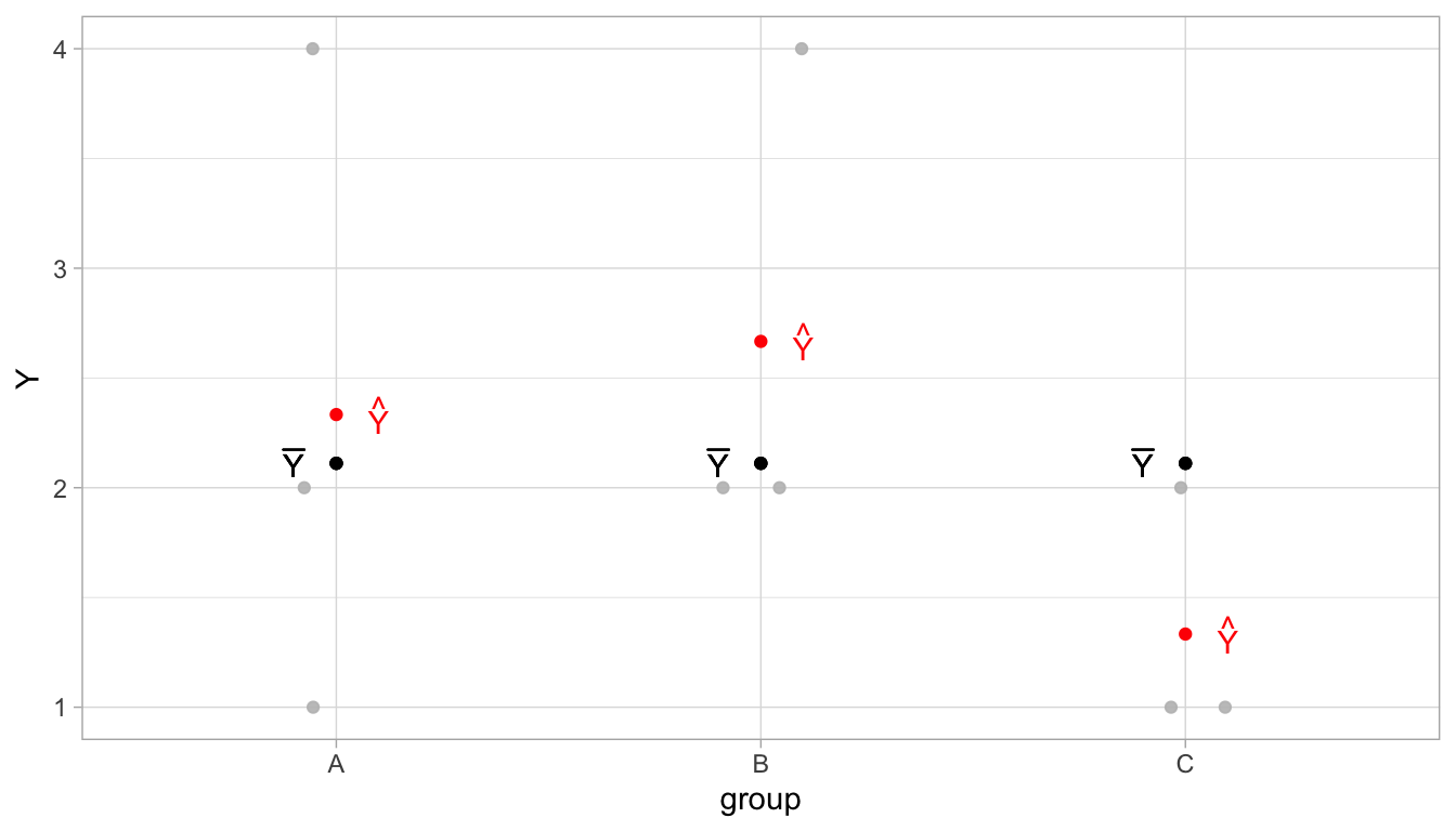
Figure 6.6: Illustration of ANOVA using a very small data set. In grey the raw data, in black the overall sample mean, and in red the sample group means.
Thus, our ANOVA model for these data is the following:
\[ \begin{eqnarray} \begin{split} Y &= b_1 \texttt{dummy}_A + b_2 \texttt{dummy}_B + b_3 \texttt{dummy}_C + e \\ e &\sim N(0, \sigma^2) \nonumber \end{split} \tag{6.3} \end{eqnarray} \]
Our OLS estimates for the parameters are the sample means, so that we have the linear equation
\[ \widehat{Y} = 2.3333333 \texttt{dummy}_A + 2.6666667 \texttt{dummy}_B + 1.3333333 \texttt{dummy}_C\]
Based on this linear equation we can determine the predicted values for
each data point. Table
6.10 shows the \(Y\)-values, the group
variable, the dummy variables from the ANOVA model equation (Equation
(6.3))
and the predicted values. We see that the predicted value for each
observed value is equal to the sample group mean.
| Y | group | dummy_A | dummy_B | dummy_C | predicted | residual |
|---|---|---|---|---|---|---|
| 1 | A | 1 | 0 | 0 | 2 | -1.33 |
| 2 | A | 1 | 0 | 0 | 2 | -0.33 |
| 4 | A | 1 | 0 | 0 | 2 | 1.67 |
| 2 | B | 0 | 1 | 0 | 3 | -0.67 |
| 2 | B | 0 | 1 | 0 | 3 | -0.67 |
| 4 | B | 0 | 1 | 0 | 3 | 1.33 |
| 2 | C | 0 | 0 | 1 | 1 | 0.67 |
| 1 | C | 0 | 0 | 1 | 1 | -0.33 |
| 1 | C | 0 | 0 | 1 | 1 | -0.33 |
Using these predicted values, we can compute the residuals, also
displayed in Table 6.10, and these help us to compute the
first estimate of \(\sigma^2\), the one based on residuals, namely the SSR
divided by the degrees of freedom. If we square the residuals in Table
6.10 and sum them, we obtain \(SSR = 8\). To
obtain the Mean Squared Error (MSE or meansq for Residuals), we divide
the SSR by the degrees of freedom. Because the linear model with 2 dummy
variables has \(n - K - 1 = 9 - 2 - 1 = 6\) residual degrees of freedom
(see Chapter @ref(chap:inf_lm)), we also have only 6 residual degrees of
freedom. Thus we get \(MSE = 8/6 = 1.3333333\). We can see these numbers
in the bottom row in the ANOVA table, displayed in Table
6.11.
| term | df | sumsq | meansq | statistic | p.value |
|---|---|---|---|---|---|
| group | 2 | 2.89 | 1.44 | 1.08 | 0.4 |
| Residuals | 6 | 8.00 | 1.33 | NA | NA |
For our second estimate of \(\sigma^2\), the one based on the group means, we look at the squared deviations of the group means from the overall mean (the grand mean). We saw that the grand mean equals 2.11. The sample mean for group A was 2.3333333, so the squared deviation equals 0.0493828. The sample mean for group B was 2.6666667, so the squared deviation equals 0.3086421. Lastly, the sample mean for group C was 1.3333333, so the squared deviation equals 0.3086421. Adding these squared deviations gives a sum of squares of 0.962963. To obtain an unbiased estimate for the population variance of these means, we have to divide this sum of squares by the number of groups minus 1 (model degrees of freedom), thus we get 0.962963/2 = 0.6604939. This we must multiply by the sample size per group to obtain an estimate of \(\sigma^2\) (see Equation (6.2)), thus we obtain 1.4444444.
| Y | group | predicted | grand_mean | deviation | sq_deviation |
|---|---|---|---|---|---|
| 1 | A | 2.33 | 2.11 | 0.22 | 0.05 |
| 2 | A | 2.33 | 2.11 | 0.22 | 0.05 |
| 4 | A | 2.33 | 2.11 | 0.22 | 0.05 |
| 2 | B | 2.67 | 2.11 | 0.56 | 0.31 |
| 2 | B | 2.67 | 2.11 | 0.56 | 0.31 |
| 4 | B | 2.67 | 2.11 | 0.56 | 0.31 |
| 2 | C | 1.33 | 2.11 | -0.78 | 0.60 |
| 1 | C | 1.33 | 2.11 | -0.78 | 0.60 |
| 1 | C | 1.33 | 2.11 | -0.78 | 0.60 |
Obtaining the estimate of \(\sigma^2\) based on the group means can also be illustrated using Table 6.12. There again we see the raw data values for variable \(Y\), the predicted values (the group means), but now also the grand mean, the deviations of the sample means from the grand mean, and their squared values. If we simply sum the squared deviations, we no longer have to multiply by sample size. Thus we have as the sum of squares 2.8888889. Then we only have to divide by the number of groups minus 1, so we have \(2.8888889/2=1.4444444\). This sum of squares, the degrees of freedom of 2, and the resulting MS can also be seen in the ANOVA table in Table 6.11.
Hence we have two estimates of \(\sigma^2\), the one called the Mean Squared Error (MSE) that is based on the residuals (sometimes also called the MS within or MSW), and the other one called the Mean Squared Between groups (MSB), that is based on the sum of squares of group mean differences. For the \(F\)-statistic, we use the MS Between (MSB) as the numerator and the MSE as the denominator,
\[F = \frac{MSB_{\texttt{group}}}{MSE} = \frac{1.4444444} {1.3333333}= 1.0833333\]
We see that the \(F\)-statistic is larger than 1. That means that the estimate for \(\sigma^2\), \(MSB_{group}\), based on the sample means is larger than the estimate based on the residuals, \(MSE\). This could indicate that the null-hypothesis, that the three population means are equal, is not true. However, is the \(F\)-value really large enough to justify such a conclusion?
To answer that question, we need to know what values the \(F\)-statistic
would take for various data sets if the null-hypothesis were true (the
sampling distribution of \(F\)). If for each data set we have three
groups, each consisting of three observed values, then we have 2 degrees
of freedom for the group effect, and 6 residual degrees of freedom.
Table 6.9
shows critical values if we want to use an \(\alpha\) of 0.05. If we look
up the column with a 2 (for the number of model degrees of freedom) and
the row with a 6 (for the residual degrees of freedom), we find a
critical \(F\)-value of 5.14. This means that if the null-hypothesis is
true and we repeatedly take random samples, we find an \(F\)-value equal
to or larger than 5.14 only 5% of the time. If we want to reject the
null-hypothesis, therefore, at an alpha of 5%, the \(F\)-value has to be
equal or larger than 5.14. Here we found an \(F\)-value of only 1.0833333,
which is much smaller, so we cannot reject the null-hypothesis that the
means are equal.
For illustration, Figure 6.7 shows the distribution of the \(F\)-statistic with 2 and 6 degrees of freedom under the null-hypothesis. The figure shows it happens quite a lot under the null-hypothesis that the \(F\)-statistic is equal to 1.0833333 or larger.
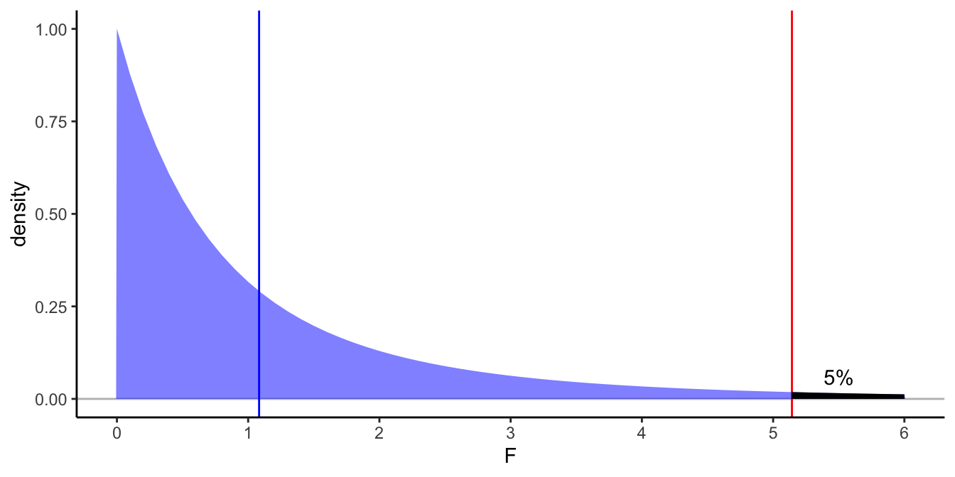
Figure 6.7: Density plot of the \(F\)-distribution with 2 and 6 degrees of freedom. In blue the observed \(F\)-statistic in the small data example, in red the critical value for an \(\alpha\) of 0.05. The blackened area under the curve is 5\(\%\).
6.11 Reporting ANOVA
In all cases where you have a categorical predictor variable with more than two categories, and where the null-hypothesis is about the equality of all group means, you have to use the factor variable in R associated with the original nominal variable. That is, don’t make dummy variables yourself, but let R do it for you. You then always report the corresponding \(F\)-statistic from the ANOVA table.
For this particular example, you report the results of the analysis of variance in the following way:
"The null-hypothesis that all 3 population means are equal was tested with an analysis of variance. The results showed that the null-hypothesis cannot be rejected, \(F(2,\ 6) = 1.08, MSE = 1.33, p = .40\)."
Always check the degrees of freedom for your \(F\)-statistic carefully. The first number refers to the degrees of freedom for the Mean Square Between: this is the number of groups minus 1 (\(K-1\)). This is equal to the number of dummy variables that are used in the linear model. This is also called the model degrees of freedom. The second number refers to the residual degrees of freedom: this is \(n - K - 1\) as we saw Chapter 5, where \(K\) is the number of dummy variables. In this ANOVA model you have 9 data points and you have 2 dummy variables for the three groups. So your residual degrees of freedom is \(9-2-1=6\). This residual degrees of freedom is equal to that of the \(t\)-statistic for multiple regression.
6.12 Relationship between \(F\)- and \(t\)-distributions
The \(t\)-distribution and the \(F\)-distribution have much in common. Here we will illustrate this. Suppose that we test the null-hypothesis that a certain population slope is 0. We perform a regression analysis and obtain a \(t\)-statistic of -2.40. Suppose our sample size was 42, so that our residual degrees of freedom equals \(42-2=40\). Figure 6.8 shows the theoretical \(t\)-distribution with 40 degrees of freedom. It also shows our value of -2.40. The shaded area represents the values for \(t\) that would be significant at an \(\alpha=0.05\).
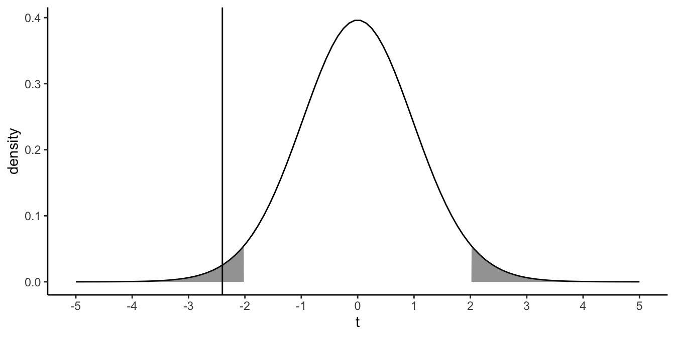
Figure 6.8: The vertical line represents a \(t\)-value of -2.40. The shaded area represents the extreme 5\(\%\) of the possible \(t\)-values
Now look closely at Figure 6.8. The density says something about the probability of drawing certain values. Imagine that you randomly pick numbers from this \(t\)-distribution. The density plot tells you that values around zero are more probable than values around 2 or -2, and that values around 2 or -2 are more probable than values around 3 or -3. Imagine that you pick a million values for \(t\), randomly from this \(t\)-distribution. Then imagine that you take the square of each value (thus, suppose as the first 3 randomly drawn \(t\)-values you get -3.12, 0.14, and -1.6, you then square these numbers to get the numbers 9.73, 0.02, and 2.79). If you then make a density plot of these one million squared numbers, you get the density plot in Figure 6.9. It turns out that this density is an \(F\)-distribution with 1 model degrees of freedom and 40 residual degrees of freedom.
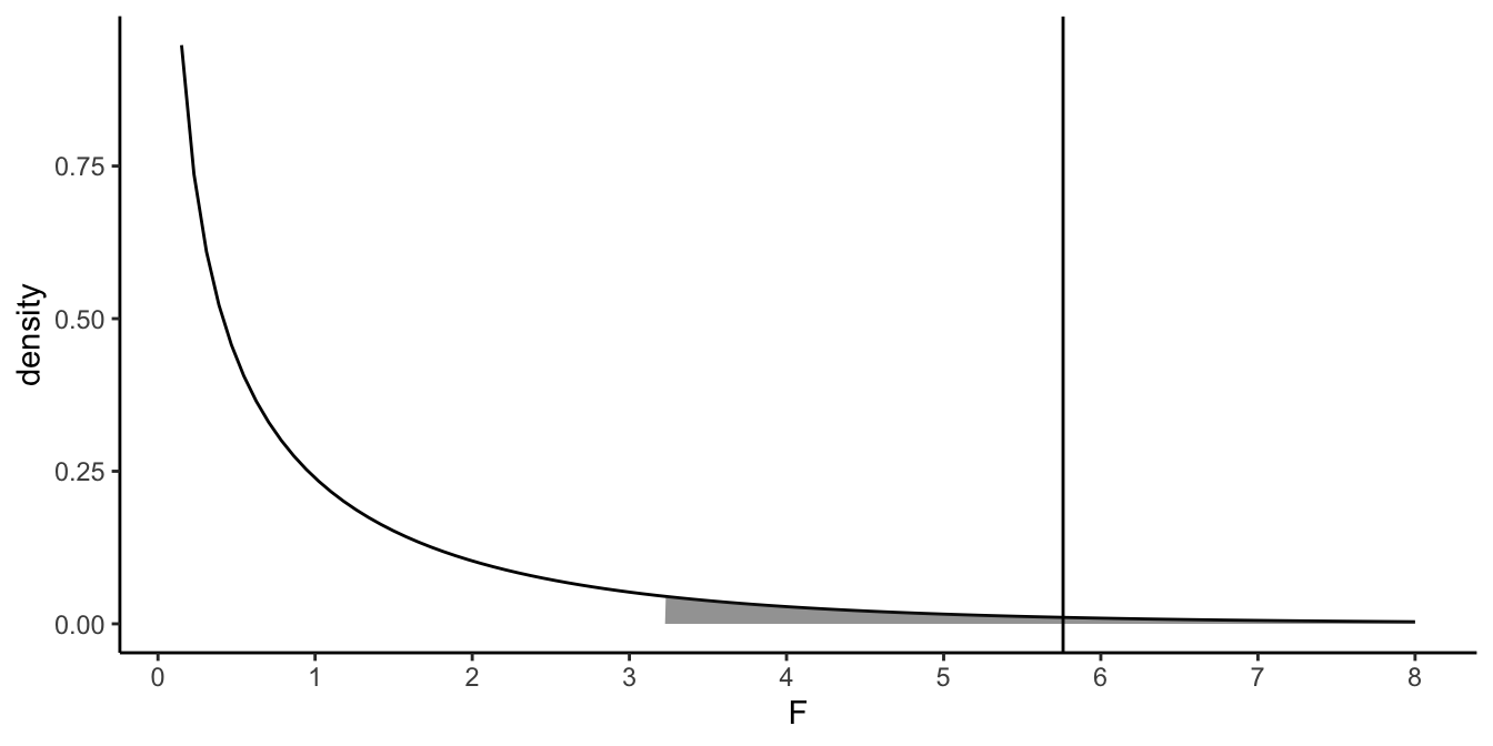
Figure 6.9: The \(F\)-distribution with 1 model degrees of freedom and 40 error degrees of freedom. The shaded area is the upper 5\(\%\) of the distribution. The vertical line represents the square of -2.40: 5.76
If we also square the observed test statistic \(t\)-value of -2.40, we obtain an \(F\)-value of 5.76. From online tables, we know that, with 1 model degrees of freedom and 40 residual degrees of freedom, the proportion of \(F\)-values larger than 5.76 equals 0.02. The proportion of \(t\)-values, with 40 (residual) degrees of freedom, larger than 2.40 or smaller than -2.40 is also 0.02. Thus, the two-sided \(p\)-value associated with a certain \(t\)-value, is equal to the (one-sided) \(p\)-value associated with an \(F\)-value that is the square of the \(t\)-value.
\[F(1, x) = t^2(x)\]
This means that if you see a \(t\)-statistic of say -2.40 reported with a residual degrees of freedom of 40, \(t(40)=-2.40\), you can equally report this as an \(F(1,\ 40)= (-2.40)^2 = 5.76\). Similarly, if you see a reported \(F\)-value of \(F(1, 67) = 49\), you could without problems turn this into a \(t(67) = 7\). Note however that this is only the case if the model degrees of freedom of the \(F\)-statistic is equal to 1. This means you cannot do this if you are comparing more than two groups means.