Chapter 7 Contrasts
7.1 Introduction
In Chapter 6 where we discussed ANOVA, we saw that we can make comparisons between means of different groups. Suppose we want to compare the mean height in three countries A, B and C. When we run a linear model, we see that usually the first group (country A) becomes the reference group. In the output then, the intercept is equal to the mean in this reference group, and the two slope parameters are the differences between countries B and A, and the difference between countries C and A, respectively. This choice of what comparisons are made, is the default choice. You may well have the desire to make other comparisons. Suppose you want to regard country C as the reference category, or perhaps you would like to make a comparison between the means of countries B and C? This chapter focuses on how to make choices regarding what comparisons you would like to make. We also explain how to do to it in R and at the same time tell you a bit more about how linear models are estimated in the first place.
7.2 The idea of a contrast
This chapter deals with contrasts. We start out by explaining what we mean with contrasts and what role they play in linear models with categorical variables. In later sections, we discuss how specifying contrasts can help us to make the standard lm() output more relevant and easier to interpret.
A contrast is a linear combination of parameters or statistics. Another word for a linear combination is a weighted sum.
Let’s focus on two sample statistics, the mean bloodpressure \(M_{Dutch}\) in a sample of two Dutch persons and the mean bloodpressure \(M_{German}\) in a sample of two German persons. We can take the sum of these two means and call it \(L1\).
\[L1 = M_{German} + M_{Dutch}\]
Note that this is equivalent to defining \(L1\) as
\[L1 = 1 \times M_{German} + 1 \times M_{Dutch}\] This is a weighted sum, where the weights for the two statistics are 1 and 1 respectively. Alternatively, you could use other weights, for example 1 and -1. Let’s call such a contrast \(L2\):
\[L2 = 1 \times M_{German} - 1 \times M_{Dutch}\] This \(L2\) could be simplified to
\[L2 = M_{German} - M_{Dutch}\] which shows that \(L2\) is then equal to the difference between the German mean and the Dutch mean. If \(L2\) is positive, it means that the German mean is higher than the Dutch mean. When \(L2\) is negative, it means that the Dutch mean is higher. We can also say that \(L2\) contrasts the German mean with the Dutch mean.
Example
If we define \(L2 = M_{German} - M_{Dutch}\) and we find that \(L2\) equals +2.13, it means that the mean of the Germans is 2.13 units higher than the mean of the Dutch. If we find a 95% confidence interval for \(L2\) of <1.99, 2.27>, this means that the best guess is that the German population mean is between 1.99 and 2.27 units higher than the Dutch population mean.
If we would fix the order of the two means \(M_{German}\) and \(M_{Dutch}\), we can make a nice short summary for a contrast. Suppose we order the groups alphabetically: first the Dutch, then the Germans. That means that we also fix the order of the weights: the first weight belongs to the group that comes first alphabetically, and the second weight belongs to the group that comes second alphabetically. Then we could summarise \(L1\) by stating only the weights: (1 1). A more common way to display these values is using a row vector:
\[ \textbf{L1} = \begin{bmatrix} 1 & 1 \end{bmatrix}\]
, representing \(1 \times M_{Dutch} + 1 \times M_{German}\). Contrast \(L2\) could be summarised as (-1 1), to represent \(-1 \times M_{Dutch} + 1\times M_{German}\). Written as a row vector we get
\[ \textbf{L2} = \begin{bmatrix} -1 & 1 \end{bmatrix}\]
We can combine these two row vectors by pasting them on top of each other and display them as a contrast matrix with 2 rows and two columns:
\[ \textbf{L} = \begin{bmatrix} \textbf{L1} \\ \textbf{L2} \end{bmatrix} = \begin{bmatrix} 1 & 1 \\ -1 & 1 \end{bmatrix}\]
In summary, a contrast is a weighted sum of group means, and can be summarised by the weights for the respective group means. Several contrasts, represented as row vectors, can be combined into a contrast matrix. Below we discuss why this simple idea of contrasts is of interest when discussing linear models. But first, let’s have a quick overview of what we learned in previous chapters.
7.3 A quick recap
Let’s briefly review what we learned earlier about linear models when dealing with categorical variables. In Chapter 4 we were introduced to the simplest linear model: a numeric dependent variable Y and one numeric independent variable X. In Chapter 6 we saw that we can also use this framework when we want to use a categorical variable X. Suppose that X has two categories, say “Dutch” and “German” to indicate the nationality of participants in a study on bloodpressure. We saw that we could create a numeric variable with only 1s and 0s that conveys the same information about nationality. Such a numeric variable with only 1s and 0s is usually called a dummy variable. Let’s use a dummy variable to code for nationality and call that variable German. All participants that are German are coded as 1 for this variable and all other participants are coded as 0. Table 7.1 shows a small imaginary data example on diastolic bloodpressure.
| participant | nationality | German | bp_diastolic |
|---|---|---|---|
| 1 | Dutch | 0 | 92 |
| 2 | German | 1 | 97 |
| 3 | German | 1 | 89 |
| 4 | Dutch | 0 | 92 |
We learned that we can plug such a dummy variable as a numeric predictor variable in a linear regression model, here with bp_diastolic (diastolic bloodpressure) as the dependent variable. The data and the OLS regression line are visualised in Figure 7.1.
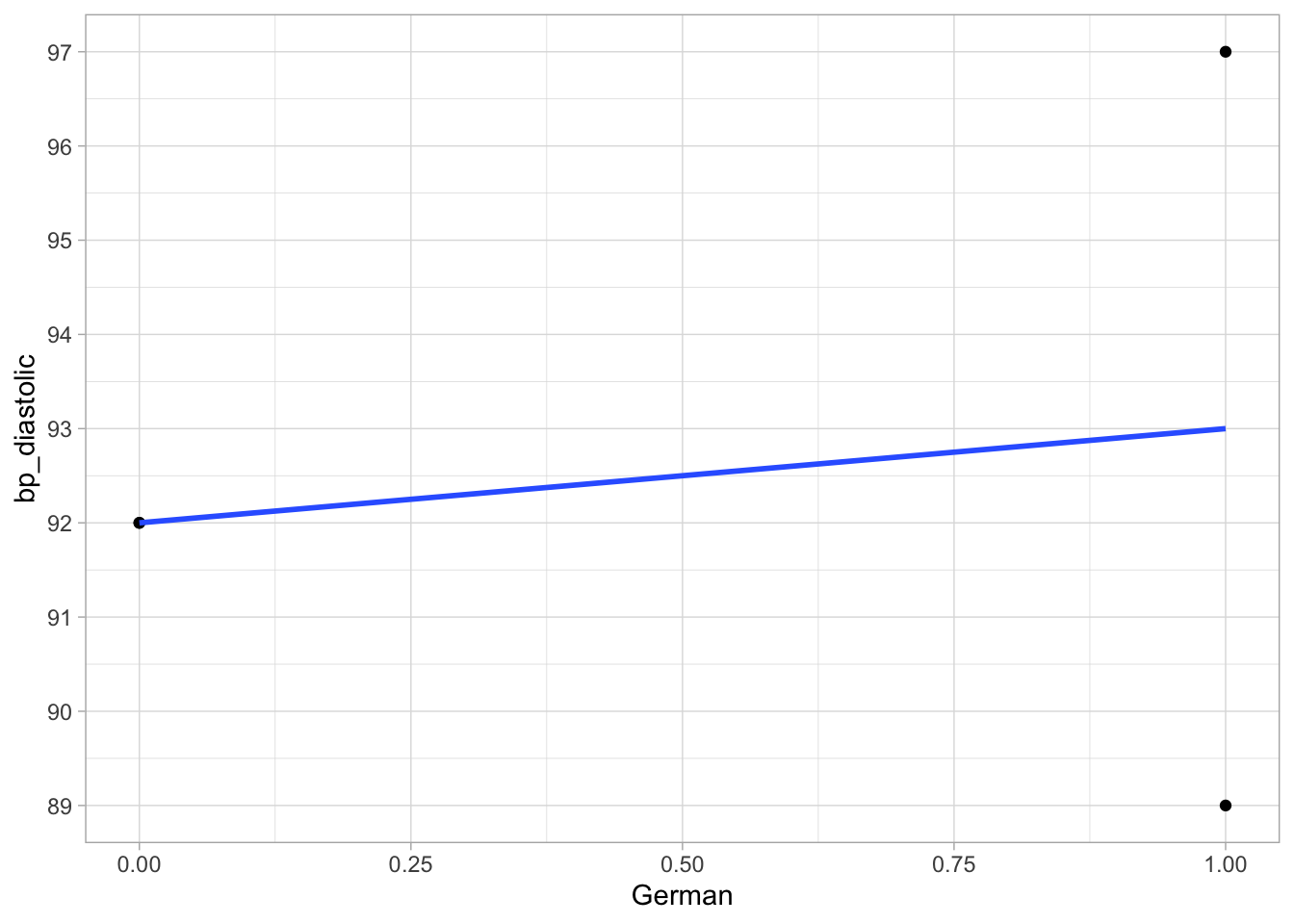
Figure 7.1: Linear regression of diastolic bloodpressure on the dummy variable German.
We learned that the slope in the model with such a dummy variable can be interpreted as the difference in the means for the two groups. In this case, the slope is equal to the difference in the means of the two groups in the sample data. The mean bloodpressure in the Dutch is \(\frac{92+92}{2}=\) 92 and in the Germans it is \(\frac{89+97}{2}=\) 93. The increase in mean bloodpressure if we move from German = 0 (Dutch) to German = 1 (German) is therefore equal to +1.
This is also what we see if R computes the regression for us, see Table 7.2.
| term | estimate | std.error | statistic | p.value |
|---|---|---|---|---|
| (Intercept) | 92 | 2.828 | 32.527 | 0.0009 |
| German | 1 | 4.000 | 0.250 | 0.8259 |
We see that being German has an effect of +1 units on the bloodpressure scale, with the individuals that are not German (Dutch) as the reference group. The intercept has the value 92 and that is the average bloodpressure in the non-German group. We can therefore view this +1 as the difference between mean German bloodpressure and mean Dutch bloodpressure.
Now suppose we do not have two groups, but three. We learned in Chapter 6 that we can have a hypothesis about the means of several groups. Suppose we have data from three groups, say Dutch, German and Italian. The data are in Table 7.3.
| participant | nationality | bp_diastolic |
|---|---|---|
| 1 | Dutch | 92 |
| 2 | German | 97 |
| 3 | German | 89 |
| 4 | Dutch | 92 |
| 5 | Italian | 91 |
| 6 | Italian | 96 |
When we run an ANOVA, the null hypothesis states that the means from the three groups are equal in the population. For example, the mean diastolic bloodpressure might be 92 for the Dutch, 93 for the Germans and 93.5 for the Italians, but this could result when the actual means in the population are the same: \(\mu_{Dutch}= \mu_{German}= \mu_{Italian}\).
If we would run an ANOVA we could get the following results
## # A tibble: 2 x 6
##   term           df sumsq meansq statistic p.value
##   <chr>       <int> <dbl>  <dbl>     <dbl>   <dbl>
## 1 nationality     2  2.33   1.17    0.0787   0.926
## 2 Residuals       3 44.5   14.8    NA       NA
We see an \(F\)-test with 2 and 3 degrees of freedom. The 2 results from the fact that we have three groups. This test is about the equality of the three group means. Compare this with the effects of the automatically created dummy variables in the lm() analysis below:
out %>% tidy()## # A tibble: 3 x 5
## term estimate std.error statistic p.value
## <chr> <dbl> <dbl> <dbl> <dbl>
## 1 (Intercept) 92.0 2.72 33.8 0.0000570
## 2 nationalityGerman 1.00 3.85 0.260 0.812
## 3 nationalityItalian 1.50 3.85 0.389 0.723In the output, the first \(t\)-test (33.8) is about the equality of the mean bloodpressure in the first group and 0. The second \(t\)-test (0.26) is about the equality of the means in groups 1 and 2, and the third \(t\)-test (0.389) is about the equality of the means in groups 1 and 3. The \(F\)-test from the ANOVA can be seen as a combination of two separate \(t\)-tests: the second and the third in this example, which are the ones about the equality of the last two group means and the first one. These two effects are from the two dummy variables created to code for the categorical variable nationality.
In the research you carry out, it is important to be clear on what you actually want to learn from the data. If you want to know if the data could have resulted from the situation where all population group means are equal, then the \(F\)-test is most appropriate. If you are more interested in whether the differences between certain countries and the first country (the reference country) are 0 in the population, the regular lm() table with the standard \(t\)-tests are more appropriate. If you are interested in other types of questions, then keep reading.
7.4 Contrasts and dummy coding
In the previous section we saw that when we run a linear model with a categorical predictor, we actually run a linear regression with a dummy variable. When the dummy varaible codes for the category German, we see that the slope is the same as the mean of the German category minus the mean of the reference group. And we see that the intercept is the same as the mean of the reference group (the non-German group). We see that the dummy variable is 1 for Germans and 0 for Dutch, and that the use of this dummy variable in the analysis results in two parameters: (1) the intercept and (2) the slope. Actually these two parameters represent two contrasts. The first parameter contrasts the difference between the Dutch mean and 0 (again, the Dutch come first alphabetically and then the weight for the Germans):
\[L1 = M_{Dutch} = M_{Dutch} - 0 = 1 \times M_{Dutch} - 0 \times M_{German} \]
In the R output, this parameter is called (Intercept). The second parameter contrasts the German mean with the Dutch mean:
\[L2 = M_{German} - M_{Dutch} = - 1 \times M_{Dutch} + 1 \times M_{German} \] This parameter is often denoted as the slope. In the R output above it is denoted as “nationalityGerman.”
These two contrasts can be represented in a contrast matrix containing two rows
\[ \textbf{L} = \begin{bmatrix} 1 & 0 \\ -1 & 1 \end{bmatrix}\]
Suppose we want to have some different output. Suppose instead we want to see in the output the mean of the Germans first and then the extra bloodpressure in the Dutch. Earlier we learned that we can get that by using a dummy variable for being Dutch, so that the German group becomes the reference group. Here, we focus on the contrasts. Suppose we want the Germans to form the reference group, then we have to estimate the contrast:
\[L3: M_{German} = 0\times M_{Dutch} + 1 \times M_{German}\]
and then we can contrast the Dutch with this reference group:
\[L4: M_{Dutch} - M_{German} = 1 \times M_{Dutch} -1 \times M_{German} \] We then have the following contrast matrix:
\[ \textbf{L} = \begin{bmatrix} 0 & 1 \\ 1 & -1 \end{bmatrix}\]
You see that when you make a choice regarding the dummy variable (either coding for being German or coding for being Dutch), this choice directly affects the contrasts that you make in the regression analysis (i.e., the output that you get). When using dummy variable German, the output gives contrasts \(L1\) and \(L2\), whereas using dummy variable Dutch leads to an output for contrasts \(L3\) and \(L4\).
To make this a bit more interesting, let’s look at a data example with 3 nationalities: Dutch, German and Italian. Suppose we want to use the German group as the reference group. We can then use the following contrast (the intercept):
\[L1: M_{German}\] Next, we are interested in the difference between the Dutch and this reference group:
\[L2 : M_{Dutch} - M_{German}\]
and the difference between the Italian and this reference group:
\[L3: M_{Italian} - M_{German}\] If we again order the three categories alphabetically, we can summarise these 3 contrasts with the contrast matrix
\[ \textbf{L} = \begin{bmatrix} 0 & 1 & 0\\ 1 & -1 & 0 \\ 0 & -1 & 1 \end{bmatrix}\]
(please check this for yourself).
Based on what we learned from previous chapters, we know we can obtain these comparisons when we compute a dummy variable for being Dutch and a dummy variable for being Italian and use these in a linear regression. We see these dummy variables Dutch and Italian in Table 7.4.
| participant | nationality | Dutch | Italian | bp_diastolic |
|---|---|---|---|---|
| 1 | Dutch | 1 | 0 | 92 |
| 2 | German | 0 | 0 | 97 |
| 3 | German | 0 | 0 | 89 |
| 4 | Dutch | 1 | 0 | 92 |
| 5 | Italian | 0 | 1 | 91 |
| 6 | Italian | 0 | 1 | 96 |
This section showed that if you change the dummy coding, you change the contrasts that you are computing in the analysis. There exists a close connection between the contrasts and the actual dummy variables that are used in an analysis. We will discuss that in the next section.
7.5 Connection between contrast and coding schemes
We saw that what dummy coding you use determines the contrasts you get in the output of a linear model. In this section we discuss this intricate connection. As we saw earlier, the contrasts can be represented as a matrix \(\mathbf{L}\) with each row representing a contrast. The way we code dummy variables, can be represented in a matrix \(\mathbf{S}\) where each column gives information about how to code a new numeric variable.
If you want the short story for how (dummy) coding and contrasts are related: matrix \(\mathbf{S}\) (the coding scheme) is the inverse of the contrast matrix \(\mathbf{L}\). That is, if you have matrix \(\mathbf{L}\) and you want to know the coding scheme \(\mathbf{S}\), you can simply ask R to compute the inverse of \(\mathbf{L}\). This also goes the other way around: if you know what coding is used, you can take the inverse of the coding scheme to determine what the output represents. If you want to know what is meant with the inverse, see advanced Section 7.5.1, although it is not strictly necessary to know it. In order to work with linear models in R, it is sufficient to know how to compute the inverse in R.
Click for more advanced material!
7.5.1 A closer look at the \(\mathbf{L}\) and \(\mathbf{S}\) matrices and their connection
By default, R orders the categories of a factor alphabetically. If we have two groups, R uses by default the following coding scheme:
\[ \textbf{S} = \begin{bmatrix} 1 & 0 \\ 1 & 1 \end{bmatrix}\]
This matrix has two rows and two columns. Each row represents a category. In our earlier example, the first category is “Dutch” and the second category is “German” (categories sorted alphabetically). Each column of the matrix \(\mathbf{S}\) represents a new numeric variable that R will compute in order to code for the categorical factor variable. The first column (representing a new numeric variable) says that for both categories (rows), the new variable gets the value 1. The second column holds a 0 and a 1. It says that the first category is coded as 0, and the second category is coded as 1.
Thus, this matrix says that we should create two new variables. They are displayed in Table 7.5, where we call them Intercept and German, respectively. Why we name the second new variable German is obvious: it’s simply a dummy variable for coding “German” as 1. Why we call the first variable Intercept is less obvious, but we will come back to that later.
| participant | nationality | Intercept | German | bp_diastolic |
|---|---|---|---|---|
| 1 | Dutch | 1 | 0 | 92 |
| 2 | German | 1 | 1 | 97 |
| 3 | German | 1 | 1 | 89 |
| 4 | Dutch | 1 | 0 | 92 |
Thus, with matrix \(\mathbf{S}\), you have all the information you need to perform a linear regression analysis with only numerical variables.
With matrix \(\mathbf{S}\) as the default, what kind of contrasts will we get, and how can we find out? It turns out that once you know \(\mathbf{S}\), you can immediately calculate (or have R calculate) what kind of contrast matrix \(\mathbf{L}\) you get. The connection between matrices \(\mathbf{L}\) and \(\mathbf{S}\) is the same as the connection between 4 and \(\frac{1}{4}\).
You might know that \(\frac{1}{4}\) is called the reciprocal of 4. The reciprocal of 4 can also be denoted by \(4^{-1}\). Thus we can write that the reciprocal of 4 is as follows:
\[4^{-1} = \frac{1}{4}\] We can say that if we have a quantity \(x\), the reciprocal of \(x\) is defined as that number when multiplied with \(x\), results in 1.
\[x x^{-1} = x^{-1} x = 1\]
Examples
- The reciprocal of 3 is equal to \(\frac{1}{3}\), because \(3 \times \frac{1}{3} = 1\).
- The reciprocal of \(\frac{1}{100}\) is equal to 100, because \(\frac{1}{100} \times 100 = 1\).
- The reciprocal of \(\frac{3}{4}\) is equal to \(\frac{4}{3}\), because \(\frac{3}{4}\times \frac{4}{3} = 1\).
Just like a number has a reciprocal, a matrix has an inverse. Similar to reciprocals, we use the “-1” to indicate the inverse of a matrix. We have that by definition, \(\mathbf{L}\mathbf{L}^{-1}=\mathbf{I}\) and \(\mathbf{S}\mathbf{S}^{-1}=\mathbf{I}\), where matrix \(\mathbf{I}\) is the matrix analogue of a 1, and its called an identity matrix. It turns out that the inverse of matrix \(\mathbf{L}\) is \(\mathbf{S}\): \(\mathbf{L}^{-1}=\mathbf{S}\), and the inverse of \(\mathbf{S}\) equals \(\mathbf{L}\): \(\mathbf{S}^{-1}=\mathbf{L}\). That implies we have that \(\mathbf{L} \mathbf{S} = \mathbf{I}\). The only difference with reciprocals is that \(\mathbf{L}\) and \(\mathbf{S}\) are matrices, so that we are in fact performing matrix algebra, which is a little bit different from algebra with single numbers. Nevertheless, it is true that if we matrix multiply \(\mathbf{L}\) and \(\mathbf{S}\), we get a matrix \(\mathbf{I}\). This matrix is as we said an identity matrix, which means it has only 1s on the diagonal (from top-left to bottom-right) and 0s elsewhere:
\[\mathbf{L}\mathbf{S} = \mathbf{S}\mathbf{L} = \mathbf{I} = \begin{bmatrix} 1 & 0 \\ 0 & 1 \end{bmatrix}\]
It turns out that if we have \(\mathbf{S}\) as defined above (the default coding scheme), the contrast matrix \(\mathbf{L}\) can only be
\[L = \begin{bmatrix} 1 & 0 \\ -1 & 1 \end{bmatrix}\]
or written in full:
\[ \mathbf{S}\mathbf{L} = \begin{bmatrix} 1 & 0 \\ 1 & 1 \end{bmatrix} \times \begin{bmatrix} 1 & 0 \\ -1 & 1 \end{bmatrix} = \begin{bmatrix} 1 & 0 \\ 0 & 1 \end{bmatrix} \]
Please note that you don’t have to know matrix algebra when studying this book, but it helps to understand what is going on when performing linear regression analysis with categorical variables. By having R do the matrix algebra for you, you can fully control what kind of output you want from an analysis.
Suppose we have matrix \(\mathbf{L}\) similar to above. We enter that matrix \(\mathbf{L}\) in R as follows:
L <- matrix(c(0,  1, 0,
              1, -1, 0,
              0, -1, 1), byrow = TRUE, nrow = 3)
L
## [,1] [,2] [,3]
## [1,] 0 1 0
## [2,] 1 -1 0
## [3,] 0 -1 1We take the inverse of \(\mathbf{L}\) to get matrix \(\mathbf{S}\) by using the ginv() function, that is given in package MASS.
library(MASS)
S <- ginv(L)
S %>% fractions() # to get more readable output
## [,1] [,2] [,3]
## [1,] 1 1 0
## [2,] 1 0 0
## [3,] 1 0 1The output is a matrix with 3 columns:
\[ \textbf{S} = \begin{bmatrix} 1 & 1 & 0\\ 1 & 0 & 0 \\ 1 & 0 & 1 \end{bmatrix}\]
This coding scheme matrix \(\mathbf{S}\) tells us what kind of variables to use to obtain these contrasts in \(\mathbf{L}\) in the output of the linear model. Each column of \(\mathbf{S}\) contains the information for each new variable. Since we have three columns, we know that we need to compute 3 variables. The first is a variable with the value 1 for all groups. We will come back to this variable of 1s later. The second is a dummy variable that codes the first group as 1 and the other two groups as 0. The third variable is also a dummy variable, coding 1 for group 3 and 0 for the other two groups.
Similarly, if you know the coding scheme, you can easily determine what the output will represent. For instance, let \(\mathbf{S}\) be the coding scheme for a dummy variable for group 1 and a dummy variable for group 2. If we enter that in R:
S <- matrix(c(1, 0,
              0, 1,
              0, 0), byrow = TRUE, nrow = 3)
For the reason explained in advanced Section 7.5.2 we add a variable of only 1s to represent the intercept.
S <- cbind(1, S)We can then determine what contrasts these variables will lead to by taking the inverse:
L <- ginv(S)
L %>% fractions() # for readability
## [,1] [,2] [,3]
## [1,] 0 0 1
## [2,] 1 0 -1
## [3,] 0 1 -1This matrix \(\mathbf{L}\) contains three rows, one for each contrast. The first row gives a contrast \(L1\) which is \(0 \times M_1 + 0 \times M_2 + 1 \times M_3\) which is equal to \(M_3\). The second row gives contrast \(1\times M_1 + 0 \times M_2 - 1\times M_3\) which amounts to the first group mean minus the last one, \(M_1 - M_3\). The third row gives the contrast \(0\times M_1 + 1 \times M_2 - 1\times M_3\) which is \(M_2 - M_3\).
Remember, contrast matrix \(\mathbf{L}\) is organised in rows, whereas coding scheme matrix \(\mathbf{S}\) is organised in columns.
With this in hand, we can first start with a contrast matrix \(\mathbf{L}\), and then we see what type of variables we should code.
Let’s return to the three-category example, with Dutch, German and Italian bloodpressure measurements. Suppose we want to have as a first contrast \(L1\), the Italian mean. Next, we we want to see the German compared to the Italian mean (\(L2\)), and last the Dutch mean compared with the Italian mean (\(L3\)).
The first contrast \(L1\) is the Italian, which, if we order alphabetically, can be written as
\[L1: M_{Italian} = M_{Italian} - 0 = 0 \times M_{Dutch} + 0\times M_{German} + 1 \times M_{Italian}\] The second contrast can be written as
\[L2: M_{German} - M_{Italian} = 0 \times M_{Dutch} + 1\times M_{German} - 1 \times M_{Italian}\] The third contrast can be written as
\[L3: M_{Dutch} - M_{Italian} = 1 \times M_{Dutch} + 0\times M_{German} - 1 \times M_{Italian}\]
These contrasts form the contrast matrix \(\mathbf{L}\):
\[ \textbf{L} = \begin{bmatrix} 0 & 0 & 1 \\ 0 & 1 & -1\\ 1 & 0 & -1 \end{bmatrix}\]
If we don’t know matrix algebra, but want to see what the inverse of this matrix is, we can type in the matrix that we want to invert:
L <- matrix(c(0, 0, 1,
              0, 1,-1,
              1, 0,-1), byrow = T, nrow = 3, ncol = 3)
L
## [,1] [,2] [,3]
## [1,] 0 0 1
## [2,] 0 1 -1
## [3,] 1 0 -1and next let R compute the inverse of \(\mathbf{L}\).
S <- ginv(L)
S %>% fractions() # simplify output
## [,1] [,2] [,3]
## [1,] 1 0 1
## [2,] 1 1 0
## [3,] 1 0 0Thus, \(\mathbf{S}\) is the inverse of the matrix with the contrasts that we want to calculate. The first column indicates a variable with only 1s for all three categories. The second column indicates that we should create a dummy variable with 1s for the second category (German) and 0s for the first category (Dutch) and the third category (Italian). The third column tells us that the third variable should consist of 1s for Dutch, 0s for Germans and 0s for Italians.
You may wonder, what is this variable with only 1s doing in this story? Didn’t we learn that we only need to compute 2 dummy variables for a categorical variable with 3 categories?
Click for more advanced material!
7.5.2 A closer look at the intercept represented as a variable with 1s
In most regression analyses, we want to include an intercept in the linear model. This happens so often that we forget that we have a choice here. For instance, in R, an intercept is included by default. For example, if you use the code with the formula bp_diastolic ~ nationality, you get the exact same result as with bp_diastolic ~ 1 + nationality. In other words, by default, R computes a variable that consists of only 1s. This can be seen if we use the model.matrix() function. This function shows the actual variables that are computed by R and used in the analysis.
lm(bp_diastolic ~ nationality, data = bloodpressure) %>%
  model.matrix()
## (Intercept) nationalityGerman nationalityItalian
## 1 1 0 0
## 2 1 1 0
## 3 1 1 0
## 4 1 0 0
## 5 1 0 1
## 6 1 0 1
## attr(,"assign")
## [1] 0 1 1
## attr(,"contrasts")
## attr(,"contrasts")$nationality
## [1] "contr.treatment"In the output, we see the actual numeric variables that are used in the analysis for the 6 observations in the data set (six rows).
We see a variable called (Intercept) with only 1s and two dummy variables, one coding for Germans, with the name nationalityGerman, and one coding for Italians with the name nationalityItalian. These variable names we see again when we look at the results of the lm() analysis:
lm(bp_diastolic ~ nationality, data = bloodpressure) %>%
  tidy()
## # A tibble: 3 x 5
## term estimate std.error statistic p.value
## <chr> <dbl> <dbl> <dbl> <dbl>
## 1 (Intercept) 92.0 2.72 33.8 0.0000570
## 2 nationalityGerman 1.00 3.85 0.260 0.812
## 3 nationalityItalian 1.50 3.85 0.389 0.723Now the names of the newly computed variables have become the names of parameters (the intercept and slope parameters). These parameter values actually represent the (default) contrasts \(L1\), \(L2\) and \(L3\), here quantified as 92.0, 1.0 and 1.5, respectively. The ‘intercept’ of 92.0 is simply the quantity that we find for the first contrast (the first row in the contrast matrix \(\mathbf{L}\)).
In summary, when you have three groups, you can invent a quantitative variable called (intercept) that is equal to 1 for all observations in your data matrix. If you then also invent a dummy variable for being German and a dummy variable for being Italian, and submit these three variables to a linear model analysis, the output will yield the mean of the Dutch, the difference between the German mean and the Dutch mean, and the difference between the Italian mean and the Dutch mean. In the code below, you see what is actually going on: the computation of the three variables and submitting these three variables to an lm() analysis. Note that R by default includes an intercept. To suppress this behaviour, we include -1 in the formula:
dummy_German   <- c(0, 1, 1, 0, 0, 0)
dummy_Italian  <- c(0, 0, 0, 0, 1, 1)
iNtErCePt      <- c(1, 1, 1, 1, 1, 1)
bp_diastolic   <- c(92, 97, 89, 92, 91, 96)

lm(bp_diastolic ~ iNtErCePt + dummy_German + dummy_Italian - 1) %>%
  tidy()
## # A tibble: 3 x 5
## term estimate std.error statistic p.value
## <chr> <dbl> <dbl> <dbl> <dbl>
## 1 iNtErCePt 92.0 2.72 33.8 0.0000570
## 2 dummy_German 1.00 3.85 0.260 0.812
## 3 dummy_Italian 1.50 3.85 0.389 0.723You see that you get the exact same results as in the default way, by specifying a categorical variable nationality:
nationality <- factor(c(1, 2, 2, 1, 3,3 ),
                      labels = c("Dutch", "German", "Italian"))

lm(bp_diastolic ~ nationality) %>%
  tidy()
## # A tibble: 3 x 5
## term estimate std.error statistic p.value
## <chr> <dbl> <dbl> <dbl> <dbl>
## 1 (Intercept) 92.0 2.72 33.8 0.0000570
## 2 nationalityGerman 1.00 3.85 0.260 0.812
## 3 nationalityItalian 1.50 3.85 0.389 0.723Or when doing the dummy coding yourself:
lm(bp_diastolic ~ dummy_German + dummy_Italian) %>%
  tidy()
## # A tibble: 3 x 5
## term estimate std.error statistic p.value
## <chr> <dbl> <dbl> <dbl> <dbl>
## 1 (Intercept) 92.0 2.72 33.8 0.0000570
## 2 dummy_German 1.00 3.85 0.260 0.812
## 3 dummy_Italian 1.50 3.85 0.389 0.723and in a way where we explicitly include an intercept of 1s:
lm(bp_diastolic ~ 1 + nationality) %>%
  tidy()
## # A tibble: 3 x 5
## term estimate std.error statistic p.value
## <chr> <dbl> <dbl> <dbl> <dbl>
## 1 (Intercept) 92.0 2.72 33.8 0.0000570
## 2 nationalityGerman 1.00 3.85 0.260 0.812
## 3 nationalityItalian 1.50 3.85 0.389 0.723lm(bp_diastolic ~ 1 + dummy_German + dummy_Italian) %>%
tidy()## # A tibble: 3 x 5
## term estimate std.error statistic p.value
## <chr> <dbl> <dbl> <dbl> <dbl>
## 1 (Intercept) 92.0 2.72 33.8 0.0000570
## 2 dummy_German 1.00 3.85 0.260 0.812
## 3 dummy_Italian 1.50 3.85 0.389 0.723with the only difference that the first parameter is now called (Intercept).
In conclusion: linear models by default include an ‘intercept’ that is actually coded as an independent variable consisting of all 1s.
7.6 Choosing the reference group in R for dummy coding
Let’s see how to run an analysis in R, when we want to control what contrasts are actually computed. This time, we want to let the Germans form the reference group, and then compare the Dutch and Italian means with the German mean.
Let’s first put the data from Table 7.3 in R, so that you can follow along using your own computer (copy the code below into an R-script).
nationality <- c("Dutch", "German", "German", "Dutch", "Italian", "Italian")
bp_diastolic <- c(92, 97, 89, 92, 91, 96)
bloodpressure <- tibble(participant, nationality, bp_diastolic)
bloodpressure
## # A tibble: 6 x 3
## participant nationality bp_diastolic
## <dbl> <chr> <dbl>
## 1 1 Dutch 92
## 2 2 German 97
## 3 3 German 89
## 4 4 Dutch 92
## 5 5 Italian 91
## 6 6 Italian 96Note that we omit dummy variables for now. Next we turn the nationality variable in the tibble bloodpressure into a factor variable. This ensures that R knows that it is a categorical variable.
bloodpressure <-
  bloodpressure %>% mutate(nationality = as.factor(nationality))
If we then look at this factor,
bloodpressure$nationality## [1] Dutch German German Dutch Italian Italian
## Levels: Dutch German Italianwe see that it has three levels. with the levels() function, we see that the first level is Dutch, the second level is German, and the third level is Italian. This is default behaviour: R chooses the order alphabetically.
levels(bloodpressure$nationality)## [1] "Dutch" "German" "Italian"This means that if we run a standard lm() analysis, the first level (the Dutch) will form the reference group, and that the two slope parameters stand for the contrasts of the bloodpressure in Germans and Italians vs the Dutch, respectively:
bloodpressure %>%
  lm(bp_diastolic ~ nationality, data = .)
##
## Call:
## lm(formula = bp_diastolic ~ nationality, data = .)
##
## Coefficients:
## (Intercept) nationalityGerman nationalityItalian
## 92.0 1.0 1.5In the case that we want to use the Germans as the reference group instead of the Dutch, we have to specify a set of contrasts that is different from this default set of contrasts.
One way to easily do this is to permanently set the reference group to another level of the nationality variable. We work with the variable nationality in the dataframe (or tibble) called bloodpressure. We use the relevel() function to change the reference group to “German.”
bloodpressure <- bloodpressure %>%
  mutate(nationality = relevel(nationality, ref = "German"))
If we check this by using the function levels() again, we see that the first group is now German, and no longer Dutch:
levels(bloodpressure$nationality)## [1] "German" "Dutch" "Italian"If we run an lm() analysis, we see from the output that the reference group is now indeed the German group (i.e., with contrasts for being Dutch and Italian).
bloodpressure %>% lm(bp_diastolic ~ nationality, data = .)##
## Call:
## lm(formula = bp_diastolic ~ nationality, data = .)
##
## Coefficients:
## (Intercept) nationalityDutch nationalityItalian
## 93.0 -1.0 0.5To check this fully, we can ask R to show us the dummy variables that it created for the analysis, using the function model.matrix().
bloodpressure %>%
  lm(bp_diastolic ~ nationality, data = .) %>%
  model.matrix()
## (Intercept) nationalityDutch nationalityItalian
## 1 1 1 0
## 2 1 0 0
## 3 1 0 0
## 4 1 1 0
## 5 1 0 1
## 6 1 0 1
## attr(,"assign")
## [1] 0 1 1
## attr(,"contrasts")
## attr(,"contrasts")$nationality
## [1] "contr.treatment"We see that R created a dummy variable for being Dutch (named nationalityDutch), and another dummy variable for being Italian (named nationalityItalian). Therefore, the reference group is now formed by the Germans. Note that R also created a variable called (Intercept), that consists of only 1s for all six individuals.
The variable nationality in the dataframe bloodpressure is now permanently altered. From now on, every time we use this variable in an analysis, the reference group will be formed by the Germans. By using mutate() and relevel() again, we can change everything back or pick another reference group.
This fixing of the reference category is very helpful in data analysis for experimental data. Suppose a researcher wants to quantify the effects of vaccine A and vaccine B on hospitalisation for COVID-19. She randomly assigns individuals to one of three groups: A, B and C, where group C is the control condition in which individuals receive a saline injection (placebo). Individuals in group A and group B get vaccines A and B, respectively. In order to quantify the effect of vaccine A, you would like to contrast group A with group C, and in order to quantify the effect of vaccine B, you would like to contrast group B with group C. In that case, it is helpful if the reference group is group C. By default, R uses the first category as the reference category, when ordered alphanumerically. By default therefore, R would choose group A as the reference group. R would then by default compute the contrast between B and A, and between C and A, apart from the mean of group A (the intercept). By changing the reference category to group C, the output would be more helpful to answer the research question.
Summary
General steps to take for using dummy coding and choosing the reference category:
- Use
levels()to check what group is named first. That group will generally be the reference group. For example, dolevels(data$variable). - If the reference group is not the right one, use
mutate()andrelevel()to change the reference group, for example do something like:data <- data %>% mutate(variable = relevel(variable, ref = "German")). - Verify with
levels()whether the right reference category is now mentioned first. Any new analysis usinglm()will now yield an analysis with dummy variables for all categories except the first one.
7.7 Alternative coding schemes
By default, R uses dummy coding. Contrasts that are computed by using dummy variables are called treatment contrasts: these contrasts are the difference between the individual groups and the reference group. Similar to defining the reference group for a particular variable (so that the first parameter value in the output is the mean of this reference group, usually termed (Intercept)), you can also set all contrasts that are used in the linear model analysis. For instance by typing
contrasts(bloodpressure$nationality)## Dutch Italian
## German 0 0
## Dutch 1 0
## Italian 0 1you see that the first variable that is created (the first column) is a dummy variable for being German, and the second variable is a dummy for being Italian. What you see in the contrast() matrix is not the contrasts per se, but the coding scheme for the new variables that are created by R. Note that the default variable with 1s (the intercept) is not displayed.
This default treatment coding (dummy coding) is fine for linear regression, but not so great for ANOVAs. We will come back to this issue in a later section when discussing moderation. For now it suffices to know that if you are interested in an ANOVA rather than a linear regression analysis, it is best to use effects coding (sometimes called sum-to-zero contrasts). Above we see that the first column after the contrasts() function (called Dutch) sums to 1, and the second column (called Italian) also sums to 1. In effects coding on the other hand, the weights for each contrast sum to 0 (hence the name sum-to-zero contrasts). Effects coding is also useful if we have specific research questions where we are interested in differences between combinations of groups. We will see in a moment what that means. Below we discuss effects coding in more detail, and also discuss other standard ways of coding (Helmert contrasts and successive differences contrast coding).
7.7.1 Effects coding
Below we will illustrate how to use and interpret a linear model when we apply effects coding. You can type along in R.
First, let’s check that we have everything in the original alphabetical order. This makes it easier to not get distracted by details.
levels(bloodpressure$nationality) # German is now the first group## [1] "German" "Dutch" "Italian"# change the order such that "Dutch" becomes the first group
bloodpressure <- bloodpressure %>%
mutate(nationality = relevel(nationality, ref = "Dutch"))
levels(bloodpressure$nationality) # Dutch is now the first group## [1] "Dutch" "German" "Italian"Next, we need to change the default dummy coding into effects coding for the nationality variable in the bloodpressure dataframe. We do that by again fixing something permanently for this variable. We use contr.sum which stands for sum-to-zero coding.
contrasts(bloodpressure$nationality) <- contr.sumWhen we run contrasts() again, we see a different set of columns, where each column now sums to 0. We no longer see dummy coding.
contrasts(bloodpressure$nationality)## [,1] [,2]
## Dutch 1 0
## German 0 1
## Italian -1 -1The values in this coding scheme matrix are used to code for the new numeric variables. The first column says that a variable should be created with 1s for Dutch, 0s for Germans and -1s for Italians. The second column indicates that another variable should be created with 0s for Dutch, 1s for Germans and -1s for Italians. Any new analysis with the variable nationality in the dataframe bloodpressure will now by default use this sum-to-zero coding scheme. If we run a linear model analysis with this factor variable, we see that we get very different values for the parameters.
bloodpressure %>%
lm(bp_diastolic ~ nationality, data = .) %>%
tidy()## # A tibble: 3 x 5
## term estimate std.error statistic p.value
## <chr> <dbl> <dbl> <dbl> <dbl>
## 1 (Intercept) 92.8 1.57 59.0 0.0000107
## 2 nationality1 -0.833 2.22 -0.375 0.733
## 3 nationality2 0.167 2.22 0.0750 0.945Let’s check that we understand how the new variables are computed.
bloodpressure %>%
lm(bp_diastolic ~ nationality, data = .) %>%
model.matrix() ## (Intercept) nationality1 nationality2
## 1 1 1 0
## 2 1 0 1
## 3 1 0 1
## 4 1 1 0
## 5 1 -1 -1
## 6 1 -1 -1
## attr(,"assign")
## [1] 0 1 1
## attr(,"contrasts")
## attr(,"contrasts")$nationality
##         [,1] [,2]
## Dutch      1    0
## German     0    1
## Italian -1 -1We still have a variable called (Intercept) with only 1s, which is used by default, as we saw earlier. There are also two other new variables, one called nationality1 and the other called nationality2, where there are 1s, 0s and -1s.
Based on this coding scheme it is hard to say what the new values in the output represent. But we saw earlier that the output values are simply the values for the contrasts, and the contrasts can be determined by taking the inverse of the coding scheme matrix \(\mathbf{S}\).
Matrix \(\mathbf{S}\) consists now of the effects coding scheme. S is therefore the same as the output of contrasts(bloodpressure$nationality).
S <- contrasts(bloodpressure$nationality)
S
## [,1] [,2]
## Dutch 1 0
## German 0 1
## Italian -1 -1We see that it has the two new numeric variables. We miss however the variable with 1s that is used by default in the analysis. If we add that we get the full matrix S with the three new variables.
S <- cbind(1, S)
S
## [,1] [,2] [,3]
## Dutch 1 1 0
## German 1 0 1
## Italian 1 -1 -1Next we take the inverse
L <- ginv(S)
L
## [,1] [,2] [,3]
## [1,] 0.3333333 0.3333333 0.3333333
## [2,] 0.6666667 -0.3333333 -0.3333333
## [3,] -0.3333333 0.6666667 -0.3333333L %>% fractions() # to make it more readable## [,1] [,2] [,3]
## [1,] 1/3 1/3 1/3
## [2,] 2/3 -1/3 -1/3
## [3,] -1/3 2/3 -1/3This gives us what we need to know about how to interpret the output. Briefly, the first parameter in the output now represents what is called the grand mean. This is the mean of all group means.
The second parameter is the difference between on the one hand the Dutch mean (the first group of the factor nationality) and on the other hand the mean of German and Italian mean, multiplied by a factor \(c = \frac{k-1}{k}\), with \(k\) being the number of groups. In this example, the number of groups equals 3, so the multiplication factor equals .
The third parameter is the difference between on the one hand the German mean (the second group of the factor nationality) and on the other hand the mean of the Dutch and Italian mean, multiplied by \(c = \frac{2}{3}\).
Let’s check whether this makes sense. Let’s get an overview of the group means in the data, and the coefficients again:
bloodpressure %>%
  group_by(nationality) %>%
  summarise(mean = mean(bp_diastolic))
## # A tibble: 3 x 2
## nationality mean
## <fct> <dbl>
## 1 Dutch 92
## 2 German 93
## 3 Italian 93.5bloodpressure %>% lm(bp_diastolic ~ nationality, data = .)##
## Call:
## lm(formula = bp_diastolic ~ nationality, data = .)
##
## Coefficients:
## (Intercept) nationality1 nationality2
## 92.8333 -0.8333 0.1667The first parameter equals 92.833 and this is equal to the grand mean \(\frac{(92 + 93 + 93.5)}{3} = 92.833\).
The second parameter equals -0.833 and this is equal to the difference between the Dutch mean 92 and the German and Italian means combined, \(\frac{(93 + 93.5)}{2} = 93.25\), so \(92 - 93.25 = -1.25\), multiplied by \(\frac{2}{3}\): \(-1.25 \times \frac{2}{3} = -0.833\). This multiplication may seem mysterious but is explained in Section @ref().
The third parameter equals 0.167 and this is indeed equal to the difference between the German mean 93 and the Dutch and Italian means combined, \(\frac{(92 + 93.5)}{2} = 92.75\), so \(93 - 92.75 = 0.25\), again multiplied by \(\frac{2}{3}\): \(0.25 \times \frac{2}{3} = 0.167\). This multiplication is also explained in Section @ref().
Even though the values themselves are a bit hard to interpret directly (because of the mysterious but explainable multiplication \(c\)), effects coding is interesting in all cases where you want to test any hypothesis about one group versus the other groups. As we saw above, the second parameter in the output is about the difference between the first group and all of the other groups (in this case groups 2 and 3). The \(t\)-test that goes along with that parameter informs us about the null-hypothesis that the first group has the same population mean as the mean of all the other group means. This is handy in a situation where you for example want to compare the control/placebo condition with the experimental conditions combined: do the various treatments in general result in a different mean than when doing nothing?
Suppose for example that we do a study on various types of therapy to quit smoking. In one group, people are put on a waiting list, in a second group people receive treatment using nicotine patches and in a third group, people receive treatment using cognitive behavioural therapy.
If your main questions are (1) what is the effect of nicotine patches on the number of cigarettes smoked, and (2) what is the effect of cognitive behavioural therapy on number of cigarettes smoked, you may want to go for the default dummy coding strategy and make sure that the control condition is the first level of your factor. The parameters and the \(t\)-tests that are relevant for your research questions are then in the second and third row of your regression table.
However, if your main question is: “Do treatments like nicotine patches and cognitive behavioural therapy help reduce the number of cigarettes smoked, compared to doing nothing?” you might want to opt for a sum-to-zero (effects coding) strategy, where you make sure that the control condition (waiting list) is the first level of your factor. The relevant null-hypothesis test for your research question is then given in the second line of your regression table (contrasting the control group with the two treatments groups).
Interpretation of effects coding output explained in more detail
Here we explain how to determine what a different coding scheme means for the interpretation of the output. It shows for example where the \(\frac{2}{3}\) comes from in the three-group example above.
We ended up with the following contrast matrix:
L %>% fractions()## [,1] [,2] [,3]
## [1,] 1/3 1/3 1/3
## [2,] 2/3 -1/3 -1/3
## [3,] -1/3 2/3 -1/3The first row represents the contrast
\[L1: 1/3 \times M_{Dutch} + 1/3 \times M_{German} + 1/3 \times M_{Italian}\]
Note that this is equivalent to the mean of the three group means (the grand mean):
\[L1: \frac{M_{Dutch} + M_{German} + M_{Italian} }{3}\] In other words, the first value we see in the output (often called intercept) will be the general mean bloodpressure averaged over these three countries. Let’s check whether that is the case. What are the mean bloodpressures in all of our three groups?
bloodpressure %>%
  group_by(nationality) %>%
  summarise(mean = mean(bp_diastolic))
## # A tibble: 3 x 2
## nationality mean
## <fct> <dbl>
## 1 Dutch 92
## 2 German 93
## 3 Italian 93.5If we take the mean of these three means, we obtain \((92 + 93 + 93.5)/3 = 92.8\) in our sample. In the output we indeed find that the first parameter value in our linear model analysis is equal to 92.8.
bloodpressure %>% lm(bp_diastolic ~ nationality, data = .)##
## Call:
## lm(formula = bp_diastolic ~ nationality, data = .)
##
## Coefficients:
## (Intercept) nationality1 nationality2
## 92.8333 -0.8333 0.1667The weights in the second row represent the second contrast:
\[L2: 2/3 \times M_{Dutch} -1/3 \times M_{German} -1/3 \times M_{Italian}\] which is equal to
\[L2: 2/3 \times ( M_{Dutch} - 1/2 \times M_{German} - 1/2 \times M_{Italian})\] In other words, \(L2\) is about the difference between on the one hand the Dutch mean and on the other hand the mean of the German and Italian means:
\[L2: 2/3 \times (M_{Dutch} - \frac{ M_{German} + M_{Italian}}{2})\] If the Dutch mean is larger than the German and Italian means combined, it means that \(L2\) will be positive. \(L2\) will be negative if the Dutch mean is below the German and Italian means combined. This \(L2\) is actually 2/3 times this difference. \(L2\) is the value displayed in the output. If we want to know the actual difference between the two means, we have to divide this value by 2/3.
If we look at the output for the second contrast, we see the value -0.833. If we divide that by 2/3 to get the actual difference in means, we obtain -1.2489. Now compare that value with the actual group means to check whether our interpretation is correct:
bloodpressure %>%
  group_by(nationality) %>%
  summarise(mean = mean(bp_diastolic))
## # A tibble: 3 x 2
## nationality mean
## <fct> <dbl>
## 1 Dutch 92
## 2 German 93
## 3 Italian 93.5We see that the German and Italian means are 93 and 93.5, respectively. We can take the mean of these two means to obtain the mean of the German and Italians combined:
(93 + 93.5) / 2## [1] 93.25which is equal to the -1.2489 above (allowing for rounding error).
The difference between the Dutch mean of 92 and this mean of 93.25 is -1.25. \(L2\) quantifies the difference in means with on the one hand the Dutch (the reference group!) and with the German and Italians means combined, multiplied by a factor 0.667. The second value in the output is therefore \(2/3 \times (M_{Dutch} - (M_{German} + M_{Italian})/2\), which is equal to \(0.667 \times -1.25 = -0.8338\). If it is large and positive it means that the Dutch mean is much larger than the other two means combined.
Now let’s look at the third contrast, which corresponds to the third parameter value in the output.
\[L3: -1/3 \times M_{Dutch} + 2/3\times M_{German} -1/3 \times M_{Italian}\]
This can be simplified to
\[L3: 2/3 \times (-0.5 \times M_{Dutch} + 1 \times M_{German} -0.5 \times M_{Italian})\] and then written as
\[L3: 2/3 \times (1 \times M_{German} -0.5 \times M_{Dutch} -0.5 \times M_{Italian})\]
which is the same as
\[L3: 2/3 \times (M_{German} - \frac{(M_{Dutch} + M_{Italian})}{2})\] In other words, \(L3\) is the difference between on the one hand the German mean and on the other hand the Dutch and Italian means combined, and then multiplied by 2/3.
In the sample means we see that the Dutch and Italian means combined is equal to \(\frac{92 + 93.5}{2} = 92.75\) and the German mean is 93. The difference between these two means is \(93 - 92.75 = 0.25\). If we multiply this by 2/3 we should get \(L3\): \(2/3 * 0.25 = 0.16675\). This is exactly what we see in the lm() output (allowing for rounding errors).
bloodpressure %>% lm(bp_diastolic ~ nationality, data = .)##
## Call:
## lm(formula = bp_diastolic ~ nationality, data = .)
##
## Coefficients:
## (Intercept) nationality1 nationality2
## 92.8333 -0.8333 0.1667If your study happens to have more than 3 groups, the multiplication factor \(c\) depends on the number of groups k: \(c = \frac{k-1}{k}\). Why this is so, can be seen if we take the example of \(k = 5\) groups. The coding scheme for sum-to-zero contrasts is generated by contr.sum. We indicate that we have 5 groups:
S <- contr.sum(5) # coding scheme matrix for 5 groups.Next we add the default variable with 1s:
S <- cbind(1, S)And then take the inverse to obtain the contrast matrix \(\mathbf{L}\):
L <- ginv(S)
L
## [,1] [,2] [,3] [,4] [,5]
## [1,] 0.2 0.2 0.2 0.2 0.2
## [2,] 0.8 -0.2 -0.2 -0.2 -0.2
## [3,] -0.2 0.8 -0.2 -0.2 -0.2
## [4,] -0.2 -0.2 0.8 -0.2 -0.2
## [5,] -0.2 -0.2 -0.2 0.8 -0.2We see in the second row that the first group is contrasted with the other 4 groups, multiplied by 0.8, which equals \(\frac{4}{5}\). In the next rows we see that each group (except the last one) is contrasted with all other groups, multiplied by \(\frac{4}{5}\). Try for yourself what the multiplication factor should be in case you have 10 groups.
In the previous section we saw that there are two different ways of carrying out a linear model analysis with categorical variables. The R default way is to use dummy coding, and the second way is effects coding. Unless you are particularly interested in an ANOVA with multiple independent categorical variables, or about combinations of groups, the default way with dummy coding is just fine.
In previous chapters we learned how to read the output from an lm() analysis when it is based on dummy coding. In the previous section we saw how to figure out what the numbers in the output represent in case of effects coding. Now we will look at a number of other alternatives of coding categorical variables, after which we will look into how to make user-specified contrasts, that help you answer your particular research question.
7.7.2 Helmert contrasts
One other well-known coding scheme is a Helmert coding scheme. We can specify we want Helmert contrasts for the nationality variable if we code the following
contrasts(bloodpressure$nationality) <- contr.helmert
contrasts(bloodpressure$nationality)
## [,1] [,2]
## Dutch -1 -1
## German 1 -1
## Italian 0 2The first column indicates how the first new variable is coded (Dutch as -1, Germans as 1 and Italians as 0), and the second column indicates a new variable with -1s for Germans and Dutch, and 2s for Italians. By default another variable is computed as 1s for all groups, representing some kind of intercept.
If we do the same trick to this matrix as before, by adding a column of 1s and then using ginv(), we get the following weights for the contrasts that we are quantifying this way
S <- cbind(1, contrasts(bloodpressure$nationality))
L <- ginv(S)
L %>% fractions()
## [,1] [,2] [,3]
## [1,] 1/3 1/3 1/3
## [2,] -1/2 1/2 0
## [3,] -1/6 -1/6 1/3Again each row gives the weights for the contrasts that are computed. Similar as with effects coding, the first contrast represents the grand mean (the mean of the group means):
\[L1: \frac{M_{German} + M_{Dutch} + M_{Italian}}{3}\]
The second row represents the difference between Dutch and German means, multiplied by 0.5:
\[L2: - \frac{1}{2} \times M_{German} + \frac{1}{2} \times M_{Dutch} + 0 \times M_{Italian}= \frac{1}{2} (M_{Dutch} - M_{German})\]
and the third row represents the difference between the Italian mean on the one hand, and the German and Dutch means combined, multiplied by 0.33.
\[ -\frac{1}{6} \times M_{Dutch} - \frac{1}{6} \times M_{German} + \frac{1}{3} \times M_{Italian} = \frac{1}{3} (M_{Italian} - \frac{M_{German} + M_{Dutch}}{2})\] In general, with a Helmert coding scheme (1) the first group is compared to the second group, (2) the first and second group combined compared to the third group, (3) the first, second and third group combined to the fourth group, and so on. Let’s imagine we have a country factor variable with 5 levels.
country <- c("A", "B", "C", "D", "E") %>% as.factor()
contrasts(country) <- contr.helmert
contrasts(country)
## [,1] [,2] [,3] [,4]
## A -1 -1 -1 -1
## B 1 -1 -1 -1
## C 0 2 -1 -1
## D 0 0 3 -1
## E 0 0 0 4then we do the trick to get the rows with the contrasts weights
S <- cbind(1, contrasts(country))
L <- ginv(S)
L %>% fractions()
## [,1] [,2] [,3] [,4] [,5]
## [1,] 1/5 1/5 1/5 1/5 1/5
## [2,] -1/2 1/2 0 0 0
## [3,] -1/6 -1/6 1/3 0 0
## [4,] -1/12 -1/12 -1/12 1/4 0
## [5,] -1/20 -1/20 -1/20 -1/20 1/5Then we see that the first contrast is the general mean. The second row is a comparison between A and B, the third one a comparison between (A+B) and C, the fourth one a comparison between (A+B+C) and D, and the fifth one a comparison between (A+B+C+D) with E. To put it differently, the Helmert contrasts compare each level with the average of the ‘preceding’ levels. Thus, we can compare categories of a variable with the mean of the preceding categories of the variable.
Helmert contrasts are useful when you have a particular logic for ordering the levels of a categorical variable. An example where a Helmert contrast might be useful is when you want to know the minimal effective dose in a dose-response study. Suppose we have a new medicine and we want to know how much of it is needed to end a headache. We split individuals with headache into four groups. In group A, people take a placebo pill, in group B people take 1 tablet of the new medicine, in group C people take 3 tablets, and in group D people take 4 tablets. In the data analysis, we first want to establish whether 1 tablet leads to a significant reduction compared to placebo. If that is not the case, we can test whether 3 tablets (group C) works better than either 1 tablet or no tablet (groups A and B combined). If that doesn’t show a significant improvement either, we may want to compare 6 tablets (group D) versus fewer tablets (groups A, B and C combined).
There are a couple of standard options in R for coding your variables. Successive differences contrast coding is also an option for meaningfully ordered categories. It compares the first level with the second level, the second level with the third level, the third level with the fourth level, and so on. The function to be used is contr.sdif. It could also be useful for a dose-response study.
One other example is contr.SAS. When used, it also computes dummy variables, but by default it will use the last category as the reference group.
Overview
Pre-set coding schemes in R
- Default is dummy coding (referring to the coding scheme \(\mathbf{S}\)), also called treatments contrasts (referring to matrix \(\mathbf{L}\)). R computes the coding scheme matrix by using
contr.treatment. With this coding, the first level of the factor variable is used as the reference group. Alternatively, withcontr.SAS, dummy coding is used with the last level of the factor variable as the reference group. - For ANOVAs, generally sum-to-zero coding is used, also called effects coding. R computes the coding scheme matrix using
contr.sum. - For categories that are ordered meaningfully, Helmert contrasts are often used. R computes the coding scheme matrix using
contr.helmert. Another option is successive differences contrast coding, usingcontr.sdif, available in theMASSpackage.
7.8 Custom-made contrasts
Sometimes, the standard contrasts are not what you are looking for. Suppose you do a wine study, where you have 10 different wines made from 10 different grapes evaluated by 10 different groups of people. Each person tastes only 1 wine and gives a score between 1 (worst quality imaginable) and 100 (best quality imaginable). Table 7.6 gives an overview of the wines made from the various grapes.
| ID | grape | origin | colour |
|---|---|---|---|
| 1 | Cabernet Sauvignon | French | Red |
| 2 | Merlot | French | Red |
| 3 | Airén | Spanish | White |
| 4 | Tempranillo | Spanish | Red |
| 5 | Chardonnay | French | White |
| 6 | Syrah (Shiraz) | French | Red |
| 7 | Garnacha (Garnache) | Spanish | Red |
| 8 | Sauvignon Blanc | French | White |
| 9 | Trebbiano Toscana (Ugni Blanc) | Italian | White |
| 10 | Pinot Noir | French | Red |
Suppose we would like to answer the following questions:
- what is the difference in quality experienced between the red and the white wines?
- what is the difference in quality experienced between French origin and Spanish origin grapes?
- what is the difference in quality experienced between the Italian origin grapes and the other two origins?
One way of addressing these questions is translating them into 3 contrasts for the factor variable ID. Suppose that the ordering of the grapes is similar to above, where Cabernet Sauvignon is the first level, Merlot is the second level, etc.
Contrast \(L1\) is about the difference between the mean of 6 red wine grapes and the mean of 4 white wine grapes:
\[L1: \frac{M_1 + M_2 + M_4 + M_6 + M_7 + M_10}{6} - \frac{M_3 + M_5 + M_8 + M_9}{4} \] This is equivalent to:
\[L1: \frac{1}{6}M_1 + \frac{1}{6}M_2 - \frac{1}{4}M_3 + \frac{1}{6}M_4 - \frac{1}{4}M_5 + \frac{1}{6}M_6 + \frac{1}{6}M_7 - \frac{1}{4}M_8 - \frac{1}{4}M_9 + \frac{1}{6}M_{10}\] We can store this contrast for the variable grape as row vector
\[\begin{bmatrix} \frac{1}{6} & \frac{1}{6} & -\frac{1}{4} & \frac{1}{6} & -\frac{1}{4} & \frac{1}{6} & \frac{1}{6} & -\frac{1}{4} & -\frac{1}{4} &\frac{1}{6} \end{bmatrix}\]
The second question can be answered by the following contrast where we have the mean of the 6 French mean ratings minus the mean of the 3 Spanish mean ratings:
\[L2: \frac{M_1 + M_2 + M_5 + M_6 + M_8 + M_10}{6} - \frac{M_3 + M_4 + M_7}{3}\] This is equivalent to
\[L2: \frac{1}{6}M_1 + \frac{1}{6}M_2 - \frac{1}{3}M_3 - \frac{1}{3}M_4 + \frac{1}{6}M_5 + \frac{1}{6}M_6 - \frac{1}{3}M_7 + \frac{1}{6}M_8 + 0 \times M_9 + \frac{1}{6}M_{10}\] We can store this contrast for the variable grape as row vector
\[\begin{bmatrix} \frac{1}{6} & \frac{1}{6} & -\frac{1}{3} &- \frac{1}{3} & \frac{1}{6} & \frac{1}{6} & -\frac{1}{3} & \frac{1}{6} & 0 &\frac{1}{6} \end{bmatrix}\]
The third question can be stated as the contrast
\[L3: M_{9} - \frac{\left(\frac{M_1 + M_2 + M_5 + M_6 + M_8 + M_{10}}{6} + \frac{M_3 + M_4 + M_7}{3}\right)} {2}\] In other words, we take the grand mean for the 6 French wines, the grand mean of the 3 Spanish wines, and take the average of these two grand means. We then contrast this grand mean with the mean rating of the single Italian wine. This contrast is equivalent to
\[L3: -\frac{1}{12}M_1 - \frac{1}{12}M_2 - \frac{1}{6}M_3 - \frac{1}{6}M_4 - \frac{1}{12}M_5 - \frac{1}{12}M_6 - \frac{1}{6}M_7 - \frac{1}{12}M_8 + 1 \times M_9 - \frac{1}{12} M_{10} \]
and can be stored in row vector
\[\begin{bmatrix} -\frac{1}{12} & -\frac{1}{12} & -\frac{1}{6} & -\frac{1}{6} & -\frac{1}{12} & -\frac{1}{12}& -\frac{1}{6} & -\frac{1}{12} & 1 & -\frac{1}{12} \end{bmatrix}\]
Combining the three row vectors, you get the contrast matrix \(\mathbf{L}\)
\[ \begin{bmatrix} \frac{1}{6} & \frac{1}{6} & -\frac{1}{4} & \frac{1}{6} & -\frac{1}{4} & \frac{1}{6} & \frac{1}{6} & -\frac{1}{4} & -\frac{1}{4} &\frac{1}{6} \\ \frac{1}{6} & \frac{1}{6} & -\frac{1}{3} &- \frac{1}{3} & \frac{1}{6} & \frac{1}{6} & -\frac{1}{3} & \frac{1}{6} & 0 &\frac{1}{6} \\ -\frac{1}{12} & -\frac{1}{12} & -\frac{1}{6} & -\frac{1}{6} & -\frac{1}{12} & -\frac{1}{12}& -\frac{1}{6} & -\frac{1}{12} & 1 & -\frac{1}{12} \end{bmatrix}\]
We can enter this matrix \(\mathbf{L}\) in R, and then compute the inverse:
l1 <- c(1/6 , 1/6  , -1/4 , 1/6 , -1/4 , 1/6 , 1/6 , -1/4 , -1/4 ,1/6)
l2 <- c(1/6 , 1/6  , -1/3 ,-1/3  , 1/6 , 1/6 , -1/3  , 1/6, 0 ,1/6 )
l3 <- c(-1/12 , -1/12  , -1/6 ,-1/6 , -1/12 , -1/12 , -1/6 , -1/12 , 1 ,-1/12)

L <- rbind(l1, l2, l3) # bind the rows together
L %>% fractions()
## [,1] [,2] [,3] [,4] [,5] [,6] [,7] [,8] [,9] [,10]
## l1 1/6 1/6 -1/4 1/6 -1/4 1/6 1/6 -1/4 -1/4 1/6
## l2 1/6 1/6 -1/3 -1/3 1/6 1/6 -1/3 1/6 0 1/6
## l3 -1/12 -1/12 -1/6 -1/6 -1/12 -1/12 -1/6 -1/12 1 -1/12S <- ginv(L) # compute the inverse
S ## [,1] [,2] [,3]
## [1,] 0.4000000000000000222045 0.3333333 0.0000000000000002220446
## [2,] 0.4000000000000001887379 0.3333333 0.0000000000000002081668
## [3,] -0.8000000000000000444089 -0.6166667 -0.3000000000000000444089
## [4,] 0.3999999999999998001599 -0.6666667 -0.0000000000000001665335
## [5,] -0.7999999999999999333866 0.3833333 -0.2999999999999999333866
## [6,] 0.4000000000000000777156 0.3333333 0.0000000000000001387779
## [7,] 0.3999999999999998001599 -0.6666667 -0.0000000000000001665335
## [8,] -0.7999999999999999333866 0.3833333 -0.2999999999999999333866
## [9,] -0.0000000000000002775558 -0.1500000 0.9000000000000000222045
## [10,] 0.4000000000000000777156 0.3333333 0.0000000000000001387779Note that we have three new variables to be computed. An intercept is missing, but R will include that by default when running a linear model.
# let's invent some data, giving two ratings for each of the 10 wines
winedata <- tibble(rating = c(70,88,81,25,59,2,93,27,32,23,13,21,8,7,76,5,57,8,20,96),
                   ID = rep(1:10, 2) %>% as.factor(),
                   grape = c("Cabernet Sauvignon",
                             "Merlot",
                             "Airén",
                             "Tempranillo",
                             "Chardonnay",
                             "Syrah (Shiraz)",
                             "Garnacha (Garnache)",
                             "Sauvignon Blanc",
                             "Trebbiano Toscana (Ugni Blanc)",
                             "Pinot Noir") %>% rep(2),
                   colour = factor(c(1, 1, 2, 1, 2, 1, 1, 2, 2, 1),
                                   labels = c("Red", "White")) %>% rep(2),
                   origin = factor(c(1, 1, 3, 3, 1, 1, 3, 1, 2, 1),
                                   labels = c("French", "Italian", "Spanish")) %>% rep(2))
Let’s look at the group means per grape:
winedata %>%
  group_by(grape) %>%
  summarise(mean = mean(rating))
## # A tibble: 10 x 2
## grape mean
## <chr> <dbl>
## 1 Airén 44.5
## 2 Cabernet Sauvignon 41.5
## 3 Chardonnay 67.5
## 4 Garnacha (Garnache) 75
## 5 Merlot 54.5
## 6 Pinot Noir 59.5
## 7 Sauvignon Blanc 17.5
## 8 Syrah (Shiraz) 3.5
## 9 Tempranillo 16
## 10 Trebbiano Toscana (Ugni Blanc) 26For the first research question, we want to estimate the difference in mean rating between the red wines and the white wines.
winedata %>%
  group_by(grape, colour) %>%
  summarise(mean = mean(rating)) %>%
  ungroup(grape) %>%
  group_by(colour) %>%
  summarise(grandmean = mean(mean))
## `summarise()` has grouped output by 'grape'. You can override using the `.groups` argument.## # A tibble: 2 x 2
## colour grandmean
## <fct> <dbl>
## 1 Red 41.7
## 2 White 38.9The grand means tell us that the difference observed in the data equals \(41.7-38.9=2.8\).
The grand means of the French and Spanish wine grapes (research question 2) are:
# computing grand means for french, spanish and italian wines
winedata %>%
  group_by(grape, origin) %>%
  summarise(mean = mean(rating)) %>%
  ungroup(grape) %>%
  group_by(origin) %>%
  summarise(grandmean = mean(mean))
## `summarise()` has grouped output by 'grape'. You can override using the `.groups` argument.## # A tibble: 3 x 2
## origin grandmean
## <fct> <dbl>
## 1 French 40.7
## 2 Italian 26
## 3 Spanish 45.2We see that the difference between the French and Spanish grand means equals \(40.7-45.2 = -4.5\).
The third question was about the Italian mean versus the mean of the grand means of the French and Spanish wines.
winedata %>%
  filter(origin == "Italian") %>%
  summarise(mean = mean(rating))   # computing the mean for the Italian wine
## # A tibble: 1 x 1
## mean
## <dbl>
## 1 26winedata %>%
filter(origin != "Italian") %>%
group_by(grape, origin) %>%
summarise(mean = mean(rating)) %>% # means per wine
ungroup(grape) %>%
group_by(origin) %>%
summarise(grandmean = mean(mean)) %>% # means of the means per wine per origin
summarise(grandgrandmean = mean(grandmean)) # the mean of the two grandmeans## `summarise()` has grouped output by 'grape'. You can override using the `.groups` argument.## # A tibble: 1 x 1
## grandgrandmean
## <dbl>
## 1 42.9The output tells us that the difference in rating of the Italian wines and the other wines combined equals \(26-42.9= -16.9\).
If we want to have information about these differences in the population, such as standard errors, confidence intervals and null-hypothesis testing, R needs the coding scheme matrix and run the linear model. We can do that by providing the \(\mathbf{S}\) matrix for the relevant factor in the analysis.
We tell R to run a linear model, with rating as the dependent variable, ID as the independent variable, and that we want to see the contrasts that are associated with coding scheme matrix \(\mathbf{S}\).
## # A tibble: 4 x 7
##   term        estimate std.error statistic  p.value conf.low conf.high
##   <chr>          <dbl>     <dbl>     <dbl>    <dbl>    <dbl>     <dbl>
## 1 (Intercept)    40.5       7.96     5.10  0.000108     23.7      57.4
## 2 ID1             2.79     16.2      0.172 0.866       -31.6      37.2
## 3 ID2            -4.50     17.8     -0.253 0.804       -42.2      33.2
## 4 ID3           -16.9      26.7     -0.634 0.535       -73.5      39.6
## [,1] [,2] [,3] [,4] [,5] [,6]
## [1,] 0.10000000 0.10000000 0.1000000 0.1000000 0.10000000 0.10000000
## [2,] 0.16666667 0.16666667 -0.2500000 0.1666667 -0.25000000 0.16666667
## [3,] 0.16666667 0.16666667 -0.3333333 -0.3333333 0.16666667 0.16666667
## [4,] -0.08333333 -0.08333333 -0.1666667 -0.1666667 -0.08333333 -0.08333333
## [,7] [,8] [,9] [,10]
## [1,] 0.1000000 0.10000000 0.0999999999999999916733 0.10000000
## [2,] 0.1666667 -0.25000000 -0.2500000000000000555112 0.16666667
## [3,] -0.3333333 0.16666667 -0.0000000000000002081668 0.16666667
## [4,] -0.1666667 -0.08333333 0.9999999999999996669331 -0.08333333In the output we see the expected values of 2.79 for research question 1, -4.50 for research question 2 and -16.9 for research question 3. In addition, we see standard errors, null-hypothesis tests and 95% confidence intervals for these contrasts.
Note that we also see an intercept that was included automatically. In order to see what it represents, we can add this intercept of 1s to S and take the inverse to obtain the contrast matrix
cbind(1, S) %>% ginv()## [,1] [,2] [,3] [,4] [,5] [,6]
## [1,] 0.10000000 0.10000000 0.1000000 0.1000000 0.10000000 0.10000000
## [2,] 0.16666667 0.16666667 -0.2500000 0.1666667 -0.25000000 0.16666667
## [3,] 0.16666667 0.16666667 -0.3333333 -0.3333333 0.16666667 0.16666667
## [4,] -0.08333333 -0.08333333 -0.1666667 -0.1666667 -0.08333333 -0.08333333
## [,7] [,8] [,9] [,10]
## [1,] 0.1000000 0.10000000 0.0999999999999999916733 0.10000000
## [2,] 0.1666667 -0.25000000 -0.2500000000000000555112 0.16666667
## [3,] -0.3333333 0.16666667 -0.0000000000000002081668 0.16666667
## [4,] -0.1666667 -0.08333333 0.9999999999999996669331 -0.08333333We see that the first row yields the grand mean over all 10 wines. You may ignore this value in the output, if it is not of interest.
You may wonder, could this not be done differently? We do not have to use the ID factor for our analysis. Perhaps it would make more sense to work with the independent variables origin and colour. Research question 1 could be answered by contrasting the categories red and white of the colour variable. Research question 2 could be answered by contrasting the categories French and Spanish of the origin variable. And the last question by contrasting the Italian categories and the French and Spanish categories together. Contrasting red with white wine could be done by using dummy coding, taking the white wine as the reference category. white comes last in the alphabet, so we could use the default contr.SAS function for the colour variable
contrasts(winedata$colour) <- contr.SASFrench comes before Italian, and Italian comes before Spanish. If we would like to compare Spanish and French with Italian, and Spanish and French with eachother, we could get these contrasts if we would use Helmert coding, with Italian as the last category, and French and Spanish as levels 1 and 2. We could accomplish this by re-specifying the origin factor variable:
winedata <- winedata %>%
  mutate(origin = factor(origin, levels = c("French", "Spanish", "Italian")))
winedata$origin  # check that Italian comes last
## [1] French French Spanish Spanish French French Spanish French Italian
## [10] French French French Spanish Spanish French French Spanish French
## [19] Italian French
## Levels: French Spanish ItalianNow make sure Helmert coding is used for this factor:
contrasts(winedata$origin) <- contr.helmert We can now run a linear model with independent factors origin and colour
winedata %>%
  lm(rating ~ colour + origin, data = .) %>%
  tidy()
## # A tibble: 4 x 5
## term estimate std.error statistic p.value
## <chr> <dbl> <dbl> <dbl> <dbl>
## 1 (Intercept) 37.9 13.0 2.93 0.00986
## 2 colour1 -1.50 17.8 -0.0843 0.934
## 3 origin1 2.25 8.89 0.253 0.804
## 4 origin2 -5.97 9.73 -0.614 0.548winedata %>%
lm(rating ~ ID, contrasts = list(ID = S), data = .) %>%
tidy()## # A tibble: 4 x 5
## term estimate std.error statistic p.value
## <chr> <dbl> <dbl> <dbl> <dbl>
## 1 (Intercept) 40.5 7.96 5.10 0.000108
## 2 ID1 2.79 16.2 0.172 0.866
## 3 ID2 -4.50 17.8 -0.253 0.804
## 4 ID3 -16.9 26.7 -0.634 0.535winedata %>%
lm(rating ~ colour + origin, data = .) %>%
model.matrix()## (Intercept) colour1 origin1 origin2
## 1 1 1 -1 -1
## 2 1 1 -1 -1
## 3 1 0 1 -1
## 4 1 1 1 -1
## 5 1 0 -1 -1
## 6 1 1 -1 -1
## 7 1 1 1 -1
## 8 1 0 -1 -1
## 9 1 0 0 2
## 10 1 1 -1 -1
## 11 1 1 -1 -1
## 12 1 1 -1 -1
## 13 1 0 1 -1
## 14 1 1 1 -1
## 15 1 0 -1 -1
## 16 1 1 -1 -1
## 17 1 1 1 -1
## 18 1 0 -1 -1
## 19 1 0 0 2
## 20 1 1 -1 -1
## attr(,"assign")
## [1] 0 1 2 2
## attr(,"contrasts")
## attr(,"contrasts")$colour
## 1
## Red 1
## White 0
##
## attr(,"contrasts")$origin
## [,1] [,2]
## French -1 -1
## Spanish 1 -1
## Italian 0 2winedata %>%
lm(rating ~ ID, contrasts = list(ID = S), data = .) %>%
model.matrix()## (Intercept) ID1 ID2 ID3
## 1 1 0.4000000000000000222045 0.3333333 0.0000000000000002220446
## 2 1 0.4000000000000001887379 0.3333333 0.0000000000000002081668
## 3 1 -0.8000000000000000444089 -0.6166667 -0.3000000000000000444089
## 4 1 0.3999999999999998001599 -0.6666667 -0.0000000000000001665335
## 5 1 -0.7999999999999999333866 0.3833333 -0.2999999999999999333866
## 6 1 0.4000000000000000777156 0.3333333 0.0000000000000001387779
## 7 1 0.3999999999999998001599 -0.6666667 -0.0000000000000001665335
## 8 1 -0.7999999999999999333866 0.3833333 -0.2999999999999999333866
## 9 1 -0.0000000000000002775558 -0.1500000 0.9000000000000000222045
## 10 1 0.4000000000000000777156 0.3333333 0.0000000000000001387779
## 11 1 0.4000000000000000222045 0.3333333 0.0000000000000002220446
## 12 1 0.4000000000000001887379 0.3333333 0.0000000000000002081668
## 13 1 -0.8000000000000000444089 -0.6166667 -0.3000000000000000444089
## 14 1 0.3999999999999998001599 -0.6666667 -0.0000000000000001665335
## 15 1 -0.7999999999999999333866 0.3833333 -0.2999999999999999333866
## 16 1 0.4000000000000000777156 0.3333333 0.0000000000000001387779
## 17 1 0.3999999999999998001599 -0.6666667 -0.0000000000000001665335
## 18 1 -0.7999999999999999333866 0.3833333 -0.2999999999999999333866
## 19 1 -0.0000000000000002775558 -0.1500000 0.9000000000000000222045
## 20 1 0.4000000000000000777156 0.3333333 0.0000000000000001387779
## attr(,"assign")
## [1] 0 1 1 1
## attr(,"contrasts")
## attr(,"contrasts")$ID
## [,1] [,2] [,3]
## 1 0.4000000000000000222045 0.3333333 0.0000000000000002220446
## 2 0.4000000000000001887379 0.3333333 0.0000000000000002081668
## 3 -0.8000000000000000444089 -0.6166667 -0.3000000000000000444089
## 4 0.3999999999999998001599 -0.6666667 -0.0000000000000001665335
## 5 -0.7999999999999999333866 0.3833333 -0.2999999999999999333866
## 6 0.4000000000000000777156 0.3333333 0.0000000000000001387779
## 7 0.3999999999999998001599 -0.6666667 -0.0000000000000001665335
## 8 -0.7999999999999999333866 0.3833333 -0.2999999999999999333866
## 9 -0.0000000000000002775558 -0.1500000 0.9000000000000000222045
## 10 0.4000000000000000777156 0.3333333 0.0000000000000001387779Overview
Using user-defined contrast in an lm() analysis
- Check the order of your levels using
levels(). - Specify your contrast vectors and combine them into a matrix \(\mathbf{L}\).
- Have R compute matrix \(\mathbf{S}\), the inverse of matrix \(\mathbf{L}\), using
ginv(). - Run the linear model, specifying that you want to use coding matrix \(\mathbf{S}\) to compute results for your contrasts, using
contrasts = list(indepvar = S)whereindepvarshould be replaced with the independent variable in your model. - R will automatically generate an intercept. Its value in the output will be the grand mean. The remaining parameters are estimates for your contrasts in \(\mathbf{L}\).
–> –> –> –> –> –> –> –> –> –> –>