Chapter 13 Generalised linear models: logistic regression
library(tidyverse)
library(knitr)
library(broom)
13.1 Introduction
In previous chapters we were introduced to the linear model, with its basic form
\[\begin{aligned} Y &= b_0 + b_1 X_1 + \dots + b_n X_n + e \\ e &\sim N(0, \sigma_e^2)\end{aligned}\]
Two basic assumptions of this model are the additivity in the parameters, and the normally distributed residual \(e\). Additivity in the parameters means that the effects of intercept and the independent variables \(X_1, X_2, \dots X_n\) are additive: the assumption is that you can sum these effects to come to a predicted value for \(Y\). So that is also true when we include an interaction effect to account for a moderation,
\[\begin{aligned} Y &= b_0 + b_1 X_1 + b_2 X_2 + b_3 X_1 X_2 + e \\ e &\sim N(0, \sigma_e^2)\end{aligned}\]
or when we use a quadratic term to account for another type of non-linearity in the data:
\[\begin{aligned} Y &= b_0 + b_1 X_1 + b_2 X_1 X_1 + e \\ e &\sim N(0, \sigma_e^2)\end{aligned}\]
In all these models, the assumption is that the effects of the parameters (\(b_0\), \(b_1\), \(b_2\)) can be summed.
The other major assumption of linear (mixed) models is the normal distribution of the residuals. As we have seen in for instance Chapter 8, sometimes the residuals are not normally distributed. Remember that with a normal distribution \(N(0,\sigma^2)\), in principle all values between \(-\infty\) and \(+\infty\) are possible, but they tend to concentrate around the value of 0, in the shape of the bell-curve. Figure 13.1 shows the normal distribution \(N(0,\sigma^2=4)\): it is centred around 0 and has variance 4. Note that the inflexion point, that is the point where the decrease in density tends to decelerate, is exactly at the values -2 and +2. These are equal to the square root of the variance, which is the standard deviation, \(-\sigma\) and \(+\sigma\).
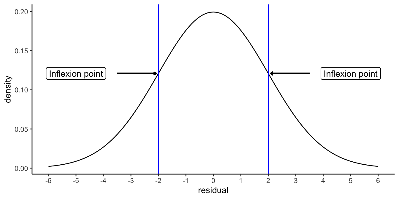
Figure 13.1: Density function of the normal distribution, with mean 0 and variance 4 (standard deviation 2). Inflexion points are positioned at residual values of minus 1 standard deviation and plus 1 standard deviation.
A normal distribution is suitable for continuous dependent variables. For most measured variables this is not true. Think for example of temperature measures: if the thermometer gives degrees Celsius with a precision of only 1 decimal, we can never have values of say 10.07 or -56.789. Our actual data will in fact be discrete, showing rounded values like 10.1, 10.2, 10.3, but never any values in between.
Nevertheless, the normal distribution can still be used in many such cases. Take for instance a data set where the temperature in Amsterdam in summer was predicted on the basis of a linear model. Fig 13.2 shows the distribution of the residuals for that model. The temperature measures were discrete with a precision of one tenth of a degree Celsius, but the distribution seems well approximated by a normal curve.
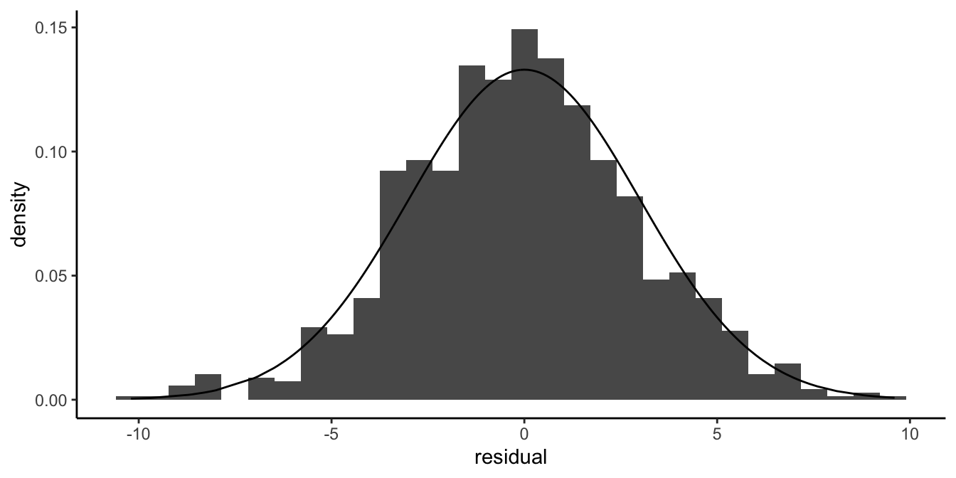
Figure 13.2: Even if residuals are really discrete, the normal distribution can be a good approximation of their distribution.
But let’s look at an example where the discreteness is more prominent. In Figure 13.3 we see the residuals of an analysis of exam results. Students had to do an assignment that had to meet 4 criteria: 1) originality, 2) language, 3) structure, and 4) literature review. Each criterion was scored as either fulfilled (1) or not fulfilled (0). The score for the assignment was determined on the basis of the number of criteria that were met, so the scores could be 0, 1, 2, 3 or 4. In an analysis, this score was predicted on the basis of the average exam score on previous assignments, using a linear model.
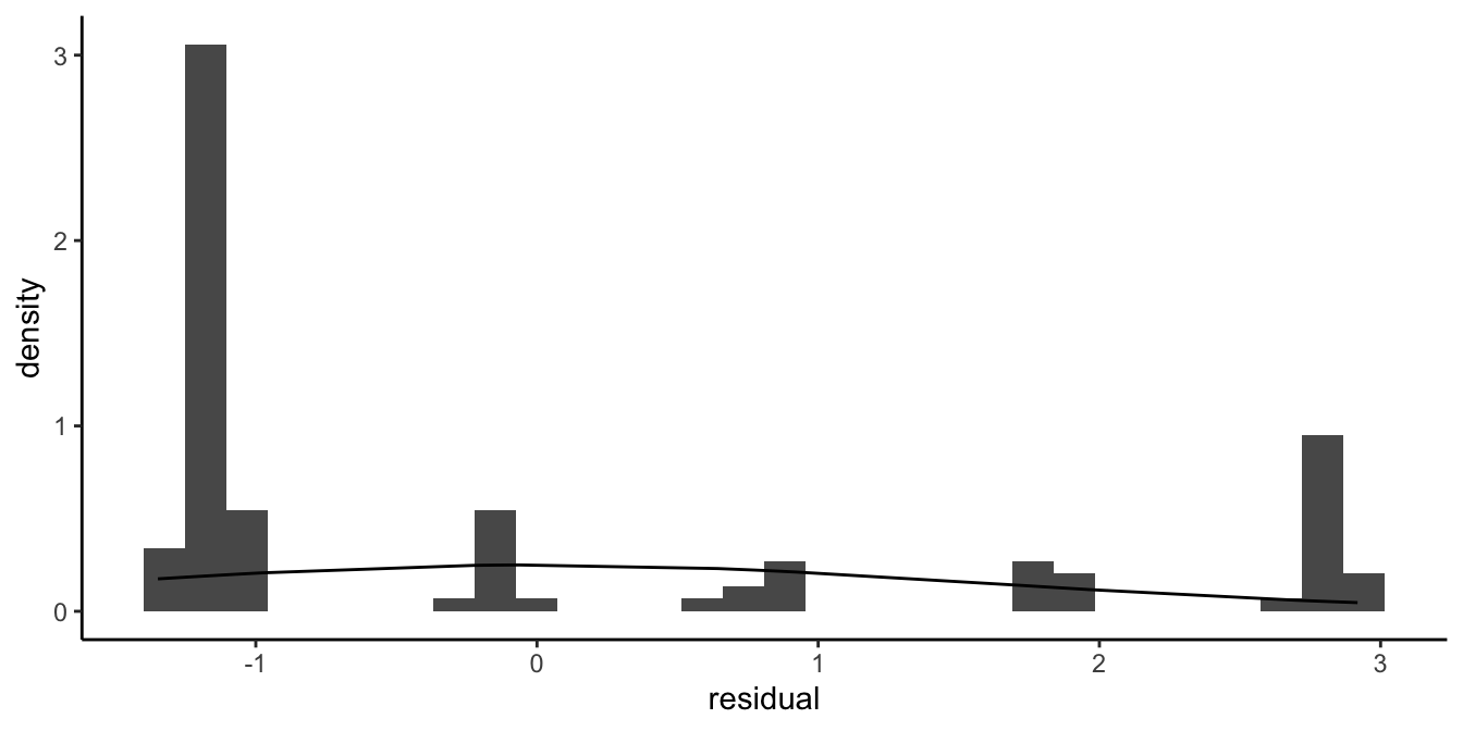
Figure 13.3: Count data example where the normal distribution is not a good approximation of the distribution of the residuals.
Figure 13.3 shows that the residuals are very discrete, and that the continuous normal distribution is a very bad approximation of the histogram. We often see this phenomenon when our data consist of counts with a limited maximum number.
An even more extreme case we observe when our dependent variable consists of whether or not students passed the assignment: only those assignments that fulfilled all 4 criteria are regarded as sufficient. If we score all students with a sufficient assignment as passed (scored as a value of 1) and all students with an insufficient assignment as failed (scored as a value of 0) and we predict this score by the average exam score on previous assignments using a linear model, we get the residuals displayed in Figure 13.4.
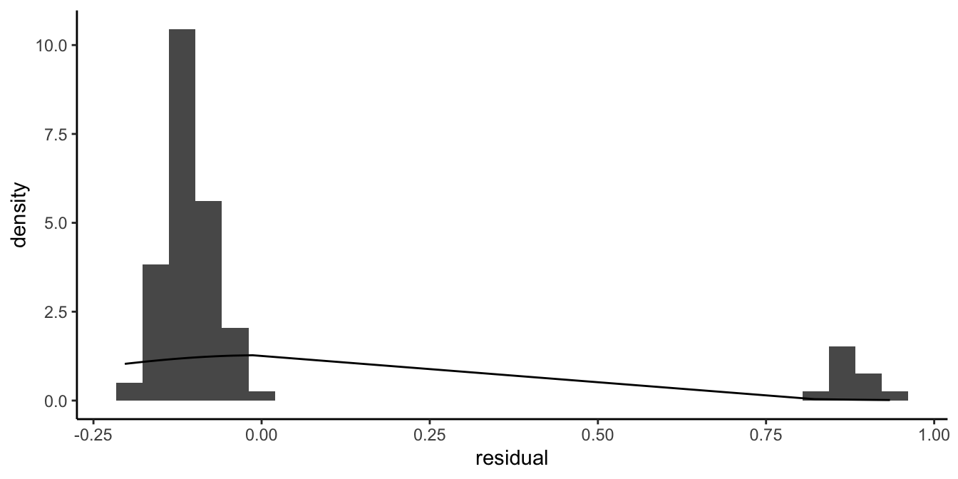
Figure 13.4: Dichotomous data example where the normal distribution is not a good approximation of the distribution of the residuals.
Here it is also evident that a normal approximation of the residuals will not do. When the dependent variable has only 2 possible values, a linear model will never work because the residuals can never have a distribution that is even remotely looking normal.
In this chapter and the next we will discuss how generalised linear models can be used to analyse data sets where the assumption of normally distributed residuals is not tenable. First we discuss the case where the dependent variable has only 2 possible values (dichotomous dependent variables like yes/no or pass/fail, heads/tails, 1/0). In Chapter 14, we will discuss the case where the dependent variable consists of counts (\(0, 1, 2, 3, 4, \dots\)).
13.2 Logistic regression
Imagine that we analyse results on an exam for third grade children. These children are usually either 6 or 7 years old, depending on what month they were born in. The exam is on February 1st. A researcher wants to know whether the age of the child can explain why some children pass the test and others fail. She computes the age of the child in months. Each child that passes the exam gets a score of 1 and all the others get a score of 0. Figure 13.5 plots the data.
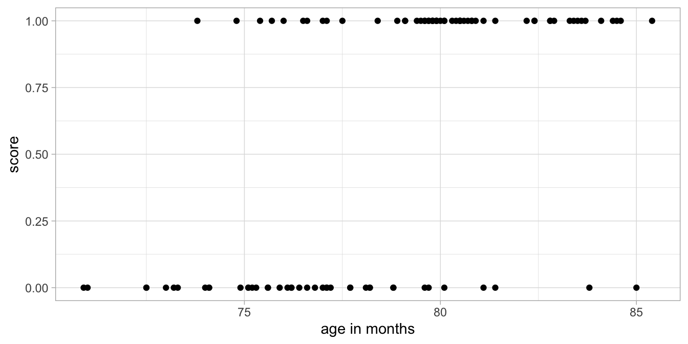
Figure 13.5: Data example: Exam outcome (score) as a function of age, where 1 means pass and 0 means fail.
She wants to use the following linear model:
\[\begin{aligned} \texttt{score} &= b_0 + b_1 \texttt{age} + e \\ e &\sim N(0, \sigma_e^2)\end{aligned}\]
Figure 13.6
shows the data with the estimated regression line and Figure
13.7 shows the
distribution of the residuals as a function of age.
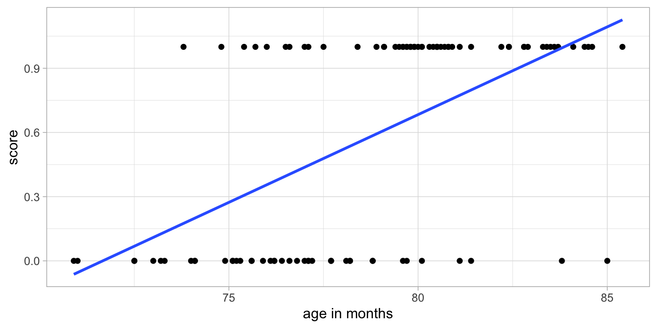
Figure 13.6: Example exam data with a linear regression line.
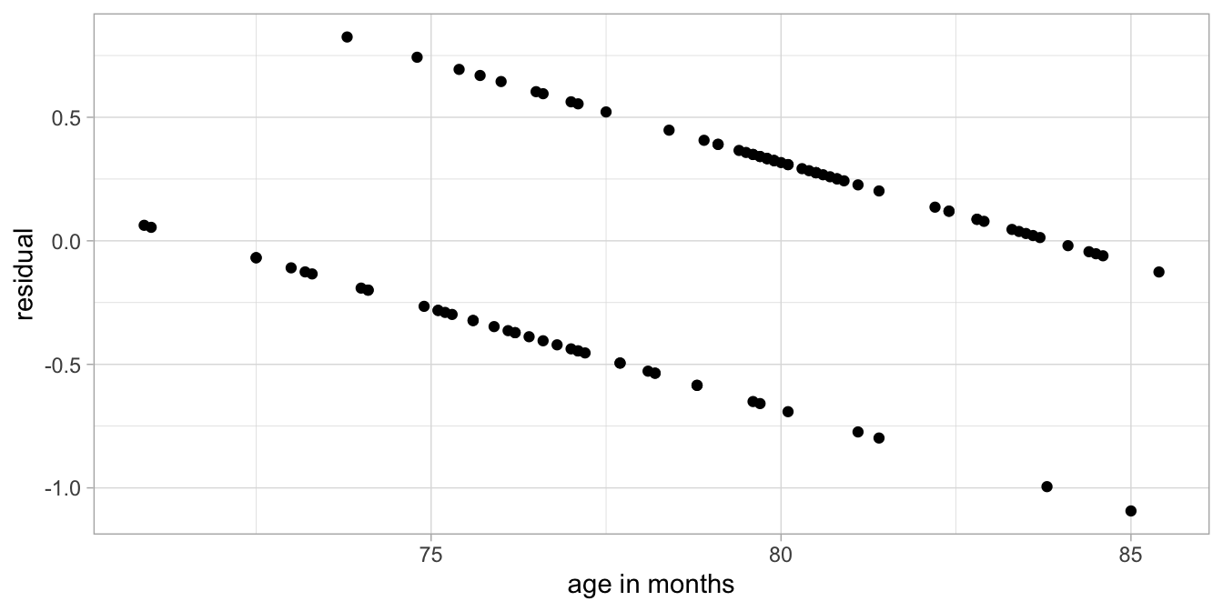
Figure 13.7: Residuals as a function of age, after a linear regression analysis of the exam data.
Clearly a linear model is not appropriate. Here, the assumption that the dependent variable, score in this case, is scattered randomly around the predicted value with a normal distribution is not reasonable. The main problem is that the dependent variable score can only have 2 values: 0 and 1. When we have a dependent variable that is categorical, so not continuous, we generally use logistic regression. In this chapter we cover the case when the dependent variable takes binary values, like 0 and 1.
13.2.1 Bernoulli distribution
Rather than using a normal distribution, we could try a Bernoulli distribution. The Bernoulli distribution is the distribution of a coin flip. For example, if the probability of heads is 0.1, we can expect that if we flip the coin 100 times, on average we expect to see 10 times heads and 90 times tails. Our best bet then is that the outcome is tails. However, if we actually flip the coin, we might see heads anyway. There is some randomness to be expected. Let \(Y\) be the outcome of a coin flip: heads or tails. If we have a Bernoulli distribution for variable \(Y\) with probability \(p\) for heads, we expect to see heads \(p\) times, but we actually observe heads or tails (\(Y\)).
\[Y \sim Bern(p)\]
The same is true for the normal distribution in the linear model case: we expect that the observed value of \(Y\) is exactly equal to its predicted value (\(b_0 + b_1 X\)), but we observe \(Y\) that it is most often different.
\[Y \sim N(\mu= b_0 + b_1 X, \sigma^2_e)\]
In our example of passing the exam by the third graders, the pass rate could also be conceived as the outcome of a coin flip: pass instead of heads and fail instead of tails. So would it be an idea to predict the probability of passing the exam on the basis of age? And then for every predicted probability, we allow for the fact that actually the observed success can differ. Our linear model could then look like this:
\[\begin{aligned} p_i &= b_0 + b_1 \texttt{age}_i \\ \texttt{score}_i &\sim Bern(p_i)\end{aligned}\]
So for each child \(i\), we predict the probability of success, \(p_i\), on the basis of her/his age. Next, the randomness in the data comes from the fact that a probability is only a probability, so that the observed success of a child \(\texttt{score}_i\), is like a coin toss with probability of \(p_i\) for success.
For example, suppose that we have a child with an age of 80 months, and we have \(b_0=-3.8\) and \(b_1=0.05\). Then the predicted probability \(p_i\) is equal to \(-3.8 + 0.05 \times 80 = 0.20\). The best bet for such a child would be that it fails the exam. But, although 0.20 is a small probability, there is a chance that the child passes the exam. This model also means that if we would have 100 children of age 80 months, we would expect that 20 of these children would pass the test and 80 would fail. But we can’t make exact predictions for one individual alone: we don’t know exactly which child will pass and which child won’t. Note that this is similar to the normally distributed residual in the linear model: in the linear model we expect a child to have a certain value for \(Y\), but we know that there will be a deviation from this predicted value: the residual. For a whole group of children with the same predicted value for \(Y\), we know that the whole group will show residuals that have a normal distribution. But we’re not sure what the residual will be for each individual child.
Unfortunately, this model for probabilities is not very helpful. If we use a linear model for the probability, this means that we can predict probability values of less than 0 and more than 1, and this is not possible for probabilities. If we use the above values of \(b_0=-3.8\) and \(b_1=0.05\), we predict a probability of -.3 for a child of 70 months and a probability of 1.2 for a child of 100 months. Those values are meaningless, since probabilities are always between 0 and 1!
13.2.2 Odds and logodds
Instead of predicting probabilities, we could predict odds. The nice property of odds is that they can have very large values, much larger than 1.
What are odds again? Odds are a different way of talking about probability. Suppose the probability of winning the lottery is 1%. Then the probability of loosing is \(99\%\). This is equal to saying that the odds of winning against loosing are 1 to 99, or \(1:99\), because the probability of winning is 99 times smaller than the probability of loosing.
As another example, suppose the probability of being alive tomorrow is equal to 0.9999. Then the probability of not being alive tomorrow is \(1-0.9999=0.0001\). Then the probability of being alive tomorrow is \(0.9999/0.0001=9999\) times larger than the the probability of not being alive. Therefore the odds of being alive tomorrow against being dead is 9999 to 1 (9999:1).
If we have a slightly biased coin, the probability of heads might be 0.6. The probability of tails is then 0.4. Then the probability of heads is then 1.5 times larger than the probability of heads (0.6/0.4=1.5). So the odds of heads against tails is then 1.5 to 1. For the sake of clarity, odds are often multiplied by a constant to get integers, so we can also say the odds of heads against tails are 3 to 2. Similarly, if the probability of heads were 0.61, the odds of heads against tails would be 0.61 to 0.39, which can be modified into 61 to 39.
Now that we know how to go from probability statements to statements about odds, how do we go from odds to probability? If someone says the odds of heads against tails is 10 to 1, this means that for every 10 heads, there will be 1 tails. In other words, if there were 11 coin tosses, 10 would be heads and 1 would be tails. We can therefore transform odds back to probabilities by noting that 10 out of 11 coin tosses is heads, so \(10/11 = 0.91\), and 1 out of 11 is tails, so \(1/11=0.09\).
If someone says the odds of winning a gold medal at the Olympics is a thousand to one (1000:1), this means that if there were \(1000+1=1001\) opportunities, there would be a gold medal in 1000 cases and failure in only one. This corresponds to a probability of 1000/1001 for winning and 1/1001 for failure.
As a last example, if at the horse races, the odds of Bruno winning
against Sacha are four to five (4:5), this means that for every 4
winnings by Bruno, there would be 5 winnings by Sacha. So out of a total
of 9 winnings, 4 will be by Bruno and 5 will be by Sacha. The
probability of Bruno outrunning Sacha is then \(4/9=0.44\).
If we would summarise the odds by doing the division, we have just one
number. For example, if the odds are 4 to 5 (4:5), the odds are
\(4/5=0.8\), and if the odds are a thousand to one (1000:1), then we can
also say the odds are 1000. Odds, unlike probabilities, can have values
that are larger than 1.
However, note that odds can never be negative: a very small odds is one to a thousand (1:1000). This can be summarised as an odds of 0.000999001, but that is still larger than 0. In summary: probabilities range from 0 to 1, and odds from 0 to infinity.
Because odds can never be negative, mathematicians have proposed to use the natural logarithm27 of the odds as the preferred transformation of probabilities. For example, suppose we have a probability of heads of 0.42. This can be transformed into an odds by noting that in 100 coin tosses, we would expect 42 times heads and 58 times tails. So the odds are 42:58, which is equal to \(\frac{42}{58}=0.7241379\). The natural logarithm of 0.7241379 equals -0.3227734 (use the ln button on your calculator!). If we have a value between 0 and 1 and we take the logarithm of that value, we always get a value smaller than 0. In short: a probability is never negative, but the corresponding logarithm of the odds can be negative.
Figure 13.8
shows the relationship between a probability (with values between 0 and
1) and the natural logarithm of the corresponding odds (the logodds).
The result is a mirrored S-shaped curve on its side. For large
probabilities close to one, the equivalent logodds becomes infinitely
positive, and for very small probabilities close to zero, the equivalent
logodds becomes infinitely negative. A logodds of 0 is equal to a
probability of 0.5. If a logodds is larger than 0, it means the
probability is larger than 0.5, and if a logodds is smaller than 0
(negative), the probability is smaller than 0.5.
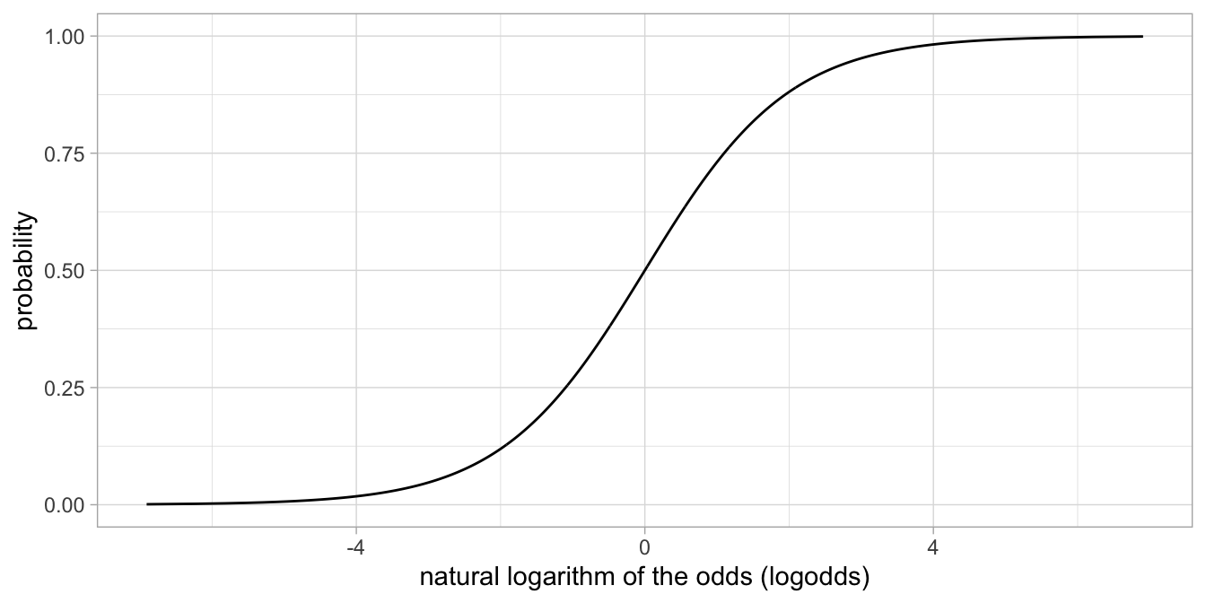
Figure 13.8: The relationship between a probability and the natural logarithm of the corresponding odds.
In summary, if we use a linear model to predict probabilities, we have the problem of predicted probabilities smaller than 0 and larger than 1 that are meaningless. If we use a linear model to predict odds we have the problem of predicted odds smaller than 0 that are meaningless: they are impossible! If on the other hand we use a linear model to predict the natural logarithm of odds (logodds), we have no problem whatsoever. We therefore propose to use a linear model to predict logodds: the natural logarithm of the odds that correspond to a particular probability.
Returning back to our example of the children passing the exam, suppose
we have the following linear equation for the relationship between age
and the logarithm of the odds of passing the exam
\[\begin{aligned} \texttt{logodds}=-33.15 + 0.42 \times \texttt{age}, \nonumber\end{aligned}\]
This equation predicts that a child aged 70 months has a logodds of \(-33.15 + 0.42 \times 70 =-3.75\). In order to transform that logodds back to a probability, we first have to take the exponential of the logodds28 to get the odds:
\[\begin{aligned} \texttt{odds} = \textrm{exp}(\texttt{logodds})= e^{\texttt{logodds}}=e^{-3.75}=0.02 \nonumber\end{aligned}\]
An odds of 0.02 means that the odds of passing the exam is 0.02 to 1 (0.02:1). So out of \(1 + 0.02= 1.02\) times, we expect 0.02 successes and 1 failure. The probability of success is therefore \(\frac{0.02}{1+0.02} = 0.02\). Thus, based on this equation, the expected probability of passing the exam for a child of 70 months equals \(0.02\).
If you find that easier, you can also memorise the following formula for the relationship between a logodds of \(x\) and the corresponding probability:
\[\begin{equation} p_x = \frac{\textrm{exp}(x)}{1+\textrm{exp}(x)} \tag{13.1} \end{equation}\]
Thus, if you have a logodds \(x\) of \(-3.75\), the odds equals \(\textrm{exp}(-3.75)=0.02\), and the corresponding probability is \(\frac{0.02}{1+0.02} = 0.02\).
13.2.3 Logistic link function
In previous pages we have seen that logodds have the nice property of having meaningful values between \(-\infty\) and \(+\infty\). This makes them suitable for linear models. In essence, our linear model for our exam data in children might then look like this:
\[\begin{aligned} \texttt{logodds}_{pass}&= b_0 + b_1 \texttt{age}\\ Y &\sim Bern(p_{pass})\end{aligned}\]
Note that we can write the odds as \(p/(1-p)\), \(p\) is a probability (or a proportion). So the logodds that corresponds to the probability of passing the exam, \(p_{pass}\), can be written as \(ln\frac{p_{pass}}{1- p_{pass}}\), so that we have
\[\begin{aligned} \textrm{ln}\frac{p_{pass}}{1- p_{pass}}&= b_0 + b_1 \texttt{age} \\ Y &\sim Bern(p_{pass})\end{aligned}\]
Note that we do not have a residual any more: the randomness around the predicted values is no longer modelled using a residual \(e\) that is normally distributed, but is now modelled by a \(Y\)-variable with a Bernoulli distribution. Also note the strange relationship between the probability parameter \(p_{pass}\) for the Bernoulli distribution, and the dependent variable for the linear equation \(b_0+b_1 age\). The linear model predicts the logodds, but for the Bernoulli distribution, we use the probability. But it turns out that this model is very flexible and useful in many real-life problems. This model is often called a logit model: one often writes that the logit of the probability is predicted by a linear model.
\[\begin{aligned} \textrm{logit}(p_{pass}) &= b_0 + b_1 \texttt{age} \\ Y &\sim Bern(p_{pass})\end{aligned}\]
In essence, the logit function transforms a \(p\)-value into a logodds:
\[\textrm{logit}(p)= \textrm{ln}( \frac{p}{1-p} ) \nonumber\]
So what does it look like, a linear model for logodds (or logits of probabilities)?
In Figure 13.9 we show a hypothetical example of a linear model for the logit of probabilities of passing an exam. These logits or logodds are predicted by age using a straight, linear regression line.
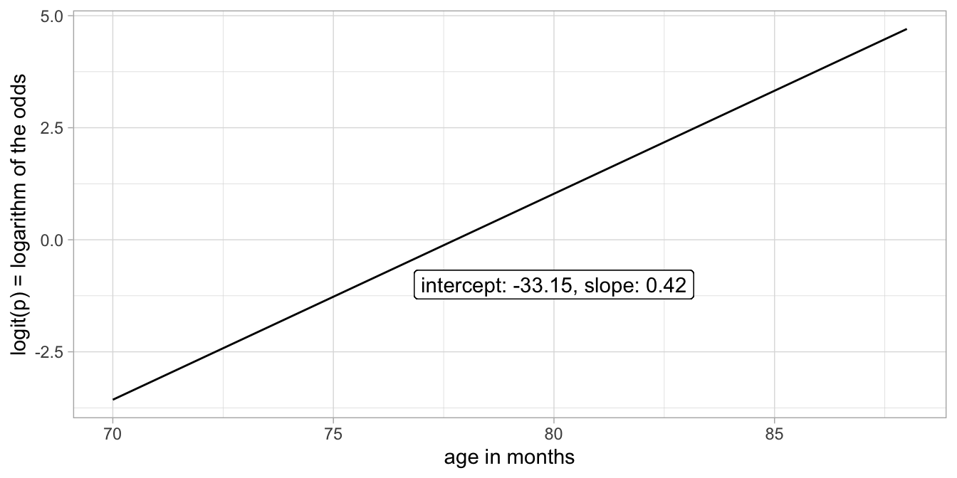
Figure 13.9: Example of a linear model for the logit of probabilities of passing an exam.
When we take all these predicted logodds and convert them back to probabilities, we obtain the plot in Figure 13.10. Note the change in the scale of the vertical axis, the rest of the plot is the same as in Figure 13.9.
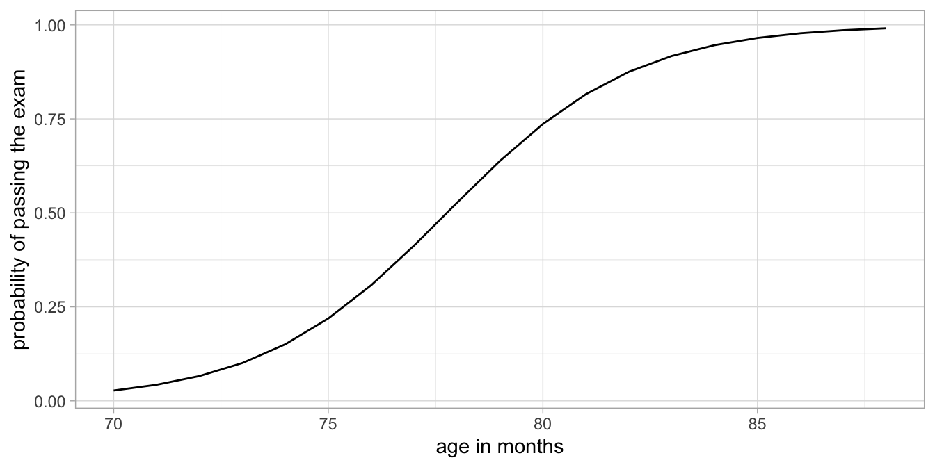
Figure 13.10: Example with logodds transformed into probabilties (vertical axis).
Here again we see the S-shape relationship between probabilities and the logodds. We see that our model predicts probabilities close to 0 for very young ages, and probabilities close to 1 for very old ages. There is a clear positive effect of age on the probability of passing the exam. But note that the relationship is not linear on the scale of the probabilities: it is linear on the scale of the logit of the probabilities, see Figure 13.9, but non-linear on the scale of the probabilities themselves, see Figure 13.10.
The curvilinear shape we see in Figure
13.10 is
called a logistic curve. It is based on the logistic function: here
\(p\) is a logistic function of age (and note the similarity with
Equation (13.1)):
\[p = \textrm{logistic}(b_0 + b_1 \texttt{age}) = \frac{\textrm{exp}(b_0 + b_1 \texttt{age})}{1+\textrm{exp}(b_0+ b_1 \texttt{age})} \nonumber\]
In summary, if we go from logodds to probabilities, we use the logistic function, \(\textrm{logistic}(x)=\frac{\textrm{exp}(x)}{1+\textrm{exp}(x)}\). If we go from probabilities to logodds, we use the logit function, \(\textrm{logit}(p)=\textrm{ln}\frac{p}{1-p}\). The logistic regression model is a generalised linear model with a logit link function, because the linear equation \(b_0 + b_1 X\) predicts the logit of a probability. It is also often said that we’re dealing with a logistic link function, because the linear equation gives a value that we have to subject to the logistic function to get the probability. Both terms, logit link function and logistic link function are used.
If we go back to our data on the third-grade children that either passed
or failed the exam, we see that this curve gives a description of our
data, see Figure 13.11. The model predicts that around the age of 78
months, the probability of passing the exam is around 0.50. We indeed
see in Figure 13.11 that around this age some children pass the exam
(score = 1) and some don’t (score = 0). On the basis of this
analysis there seems to be a positive relationship between age in
third-grade children and the probability of passing the exam in this
sample.
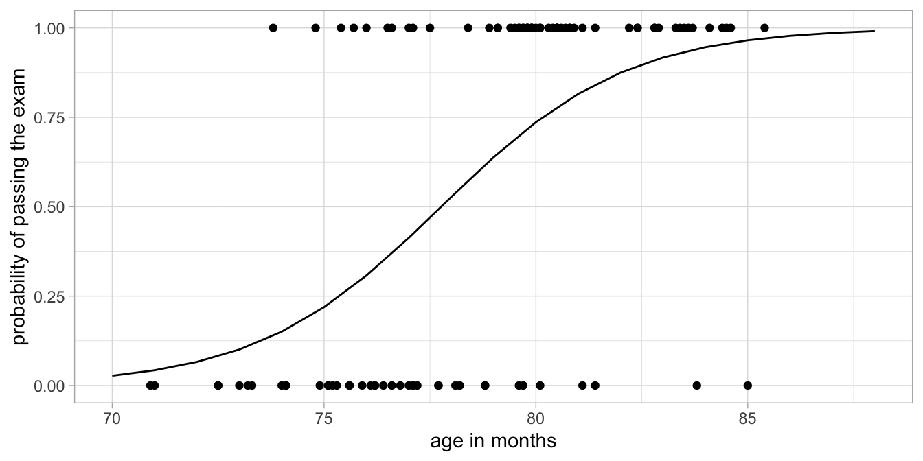
Figure 13.11: Transformed regression line and raw data points.
What we have done here is a logistic regression of passing the exam on age. It is called logistic because the curve in Figure 13.11 has a logistic shape. Logistic regression is one specific form of a generalised linear model. Here we have applied a generalised linear model with a so-called logit link function: instead of modelling dependent variable \(Y\) directly, we have modelled the logit of the probabilities of obtaining a \(Y\)-value of 1. There are many other link functions possible. One of them we will see in the chapter on generalised linear models for count data (Chapt. 14). But first, let’s see how logistic regression can be performed in R, and how we should interpret the output.
| train | age | sex_male | income | business |
|---|---|---|---|---|
| 1 | 35.11738 | 1 | 7544 | 1 |
| 1 | 66.66322 | 1 | 7096 | 0 |
| 0 | 42.76555 | 1 | 29261 | 1 |
| 0 | 72.63010 | 0 | 24977 | 0 |
| 1 | 76.24944 | 0 | 876 | 1 |
| 0 | 19.87006 | 1 | 126943 | 1 |
13.3 Logistic regression in R
Imagine a data set on travellers from Amsterdam to Paris. From 1000
travellers, randomly sampled in 2017, we know whether they took the
train to Paris, or whether they used other means of transportation. Of
these travellers, we know their age, sex, yearly income, and whether
they are travelling for business or not. Part of the data are displayed
in Table 13.1. A score of 1 on the variable train means they
took the train, a score of 0 means they did not.
Suppose we want to know what kind of people are more likely to take the train to Paris. We can use a logistic regression analysis to predict whether people take the train or not, on the basis of their age, sex, income, and main purpose of the trip.
Let’s see whether income predicts the probability of taking the train.
The function that we use in R is the glm() function, which stands for
Generalised Linear Model. We can use the following code:
model.train <- data.train %>%
glm(train ~ income,
data = .,
family = binomial(link = logit))
train is our dependent variable, income is our independent variable,
and these variables are stored in the data frame called data.train.
But further we have to specify that we want to use the Bernoulli
distribution and a logit link function. So link = logit. But why a
binomial distribution? Well, the Bernoulli distribution (one coin flip)
is a special case of the Binomial distribution (the distribution of
several coin flips). So here we use a binomial distribution for one coin
flip, which is equivalent to a Bernoulli distribution. Actually, the
code can be a little bit shorter, because the logit link function is the
default option with the binomial distribution:
model.train <- data.train %>%
glm(train ~ income,
data = .,
family = binomial)
Below, we see the parameter estimates from this generalised linear model run on the train data.
model.train %>%
  tidy()
## # A tibble: 2 x 5
## term estimate std.error statistic p.value
## <chr> <dbl> <dbl> <dbl> <dbl>
## 1 (Intercept) 90.0 32.5 2.77 0.00564
## 2 income -0.00817 0.00297 -2.75 0.00603The parameter estimates table from a glm() analysis looks very much
like that of the ordinary linear model and the linear mixed model. An
important difference is that the statistics shown are no longer
\(t\)-statistics, but \(z\)-statistics. This is because with logistic
models, the ratio \(b_1/SE\) does not have a \(t\)-distribution. In ordinary
linear models, the ratio \(b_1/SE\) has a \(t\)-distribution because in
linear models, the variance of the residuals, \(\sigma^2_e\), has to be
estimated (as it is unknown). If the residual variance were known,
\(b_1/SE\) would have a standard normal distribution. In logistic models,
there is no \(\sigma^2_e\) that needs to be estimated (it is by default
1), so the ratio \(b_1/SE\) has a standard normal distribution. One could
therefore calculate a \(z\)-statistic \(z=b_1/SE\) and see whether that
value is smaller than 1.96 or larger than 1.96, if you want to test with
a Type I error rate of 0.05.
The interpretation of the slope parameters is very similar to other
linear models. Note that we have the following equation for the logistic
model:
\[\begin{aligned} \textrm{logit}(p_{\texttt{train}}) &= b_0 + b_1 \texttt{income} \nonumber \\ \texttt{train} &\sim Bern(p_{\texttt{train}})\end{aligned}\]
If we fill in the values from the R output, we get
\[\begin{aligned} \textrm{logit}(p_{\texttt{train}}) &= 90.0 - 0.008 \times \texttt{income} \nonumber \\ \texttt{train} &\sim Bern(p_{\texttt{train}})\end{aligned}\]
We can interpret these results by making some predictions. Imagine a traveller with a yearly income of 11,000 Euros. Then the predicted logodds equals \(90.0 - 0.00817 \times 11000= 0.13\). When we transform this back to a probability, we get \(\frac{\textrm{exp}(0.13) } {1+ \textrm{exp}(0.13) }= 0.53\). So this model predicts that for people with a yearly income of 11,000, about 53% of them take the train (if they travel at all, that is!).
Now imagine a traveller with a yearly income of 100,000. Then the predicted logodds equals \(90.0 - 0.00817 \times 100000 = -727\). When we transform this back to a probability, we get \(\frac{\textrm{exp}(-727) } {1+ \textrm{exp}(-727) }= 0.00\). So this model predicts that for people with a yearly income of 100,000, close to none of them take the train. Going from 11,000 to 100,000 is a big difference. But the change in probabilities is also huge: the probability goes down from 0.53 to 0.00.
We found a difference in probability of taking the train for people with different incomes in this sample of 1000 travellers, but is there also an effect of income in the entire population of travellers between Amsterdam and Paris? The regression table shows us that the effect of income, \(- 0.00817\), is statistically significant at an \(\alpha\) of 5%, \(z = -2.75, p = .006\).
"In a logistic regression with dependent variable taking the train and independent variable income, the null-hypothesis was tested that income is not related to whether people take the train or not. Results showed that the null-hypothesis could be rejected, \(b_{income} = -0.00817, z = -2.75, p = .006\). We conclude that in the population of travellers to Paris, a higher income is associated with a lower probability of travelling by train."
Note that similar to other linear models, the intercept can be interpreted as the predicted logodds for people that have values 0 for all other variables in the model. Therefore, an intercept of 90.0 means in this case that the predicted logodds for people with zero income equals 90.0. This is equivalent to a probability very close to 1.
The natural logarithm of a number is its logarithm to the base of the constant \(e\), where \(e\) is approximately equal to 2.7. The natural logarithm of \(x\) is generally written as \(\textrm{ln} x\) or \(\textrm{log}^e x\). The natural logarithm of \(x\) is the power to which \(e\) needs to be raised to equal \(x\). For example, \(\textrm{ln}(2)\) is 0.69, because \(e^{0.69} = 2\), and \(\textrm{ln}(0.2)=-1.6\) because \(e^{-1.6}=0.2\). The natural logarithm of \(e\) itself, \(\textrm{ln}(e)\), is 1, because \(e^1 = e\), while the natural logarithm of 1, \(\textrm{ln}(1)\), is 0, since \(e^0 = 1\).↩︎
If we know \(\textrm{ln}(x)=60\), we have to infer that \(x\) equals \(e^{60}\), because \(\textrm{ln}(e^{60})=60\) by definition of the natural logarithm, see previous footnote. Therefore, if we know that \(\textrm{ln}(x)=c\), we know that \(x\) equals \(e^c\). The exponent of \(c\), \(e^c\), is often written as \(\textrm{exp}(c)\). So if we know that the logarithm of the odds equals \(c\), \(\texttt{logodds}=\textrm{ln}(\texttt{oddsratio})=c\), then the odds is equal to \(\textrm{exp}(c)\).↩︎