Chapter 10 Lab 8 - 03/12/2021
In this lecture: - we give some hint on Rmarkdown and how you must know it to perform the exam PSBF - we study multiple linear regression in R
10.1 RMarkdown
RMarkdown is the best framework for data science (official website: https://rmarkdown.rstudio.com/). It makes it possible to obtain reproducible reports that include text, R code and the corresponding output. See this video for an introduction to RMarkdown: https://vimeo.com/178485416. To use RMarkdown you have to install the rmarkdown and knitr package.
For the exercise part of the PBSF exam you will receive a RMarkdown document, i.e. a file with .Rmd extension (see for example the file PSBF_Exam_FacSimile.Rmd available in the PSBF Moodle page). You can open the file (by double clicking) with RStudio.
In the top part of the file, as shown in Figure 10.1, you just have to write your Surname, Name and Student ID. The rest must not be modified. You can compile the RMarkdown file to obtain an html file by using the Knit button, see the yellow circle in Figure 10.1. If the compilation concludes correctly a web page will be opened with your html document. Moreover, the file PSBF_Exam_FacSimile.html will be saved in the same folder. If you want to see the web page directly in the bottom right panel of RStudio click on the wheel button (see the purple circle in Figure 10.1) and select Preview in Viewer Pane (then compile again your document with Knit, you will see your document in the Viewer pane).
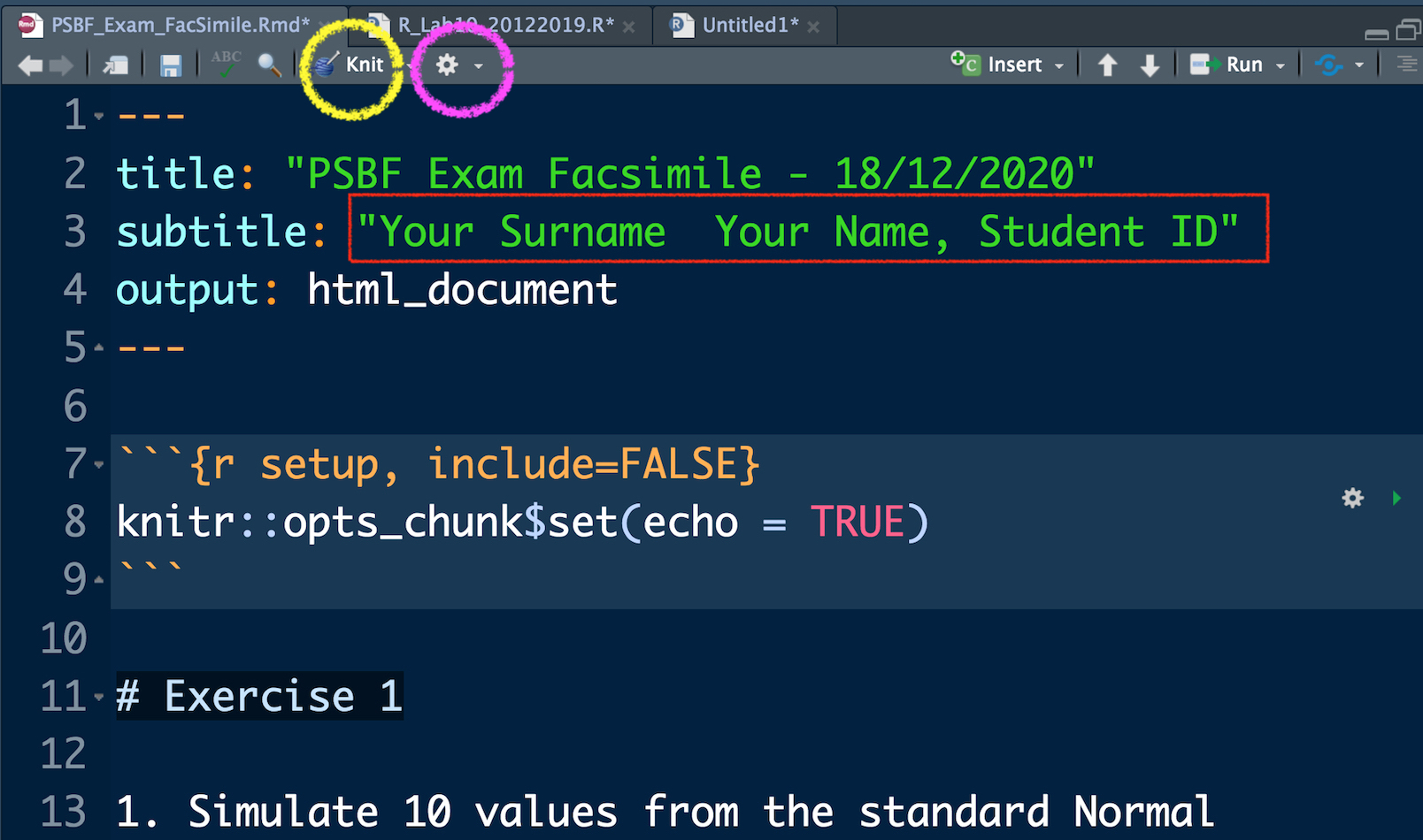
Figure 10.1: Top part of the RMarkdown file
In Figure 10.2 you can view the beginning of Exercise 1 (see the purple rectangle) and the first sub-exercise (1.). This must not be modified. You have instead to write your code and your comments (preceded by #) in the yellow area delimited by the symbols ```{r} and ``` (this area is known as code chunk). To check what your code produces you can:
- run separately each line of code by using Ctrl/Cmd Enter. This is the approach you have used so far, you will find your results in the console and the new objects in your environment (see top right panel).
- Use the arrow located in the right part of the code chunk (see the orange arrow in Figure 10.2 ). This will run all the code lines included in the chunk. You will find your results in the console and the new objects in your environment (see top right panel).
In any case you have to compile your document (using the Knit button) after each sub-exercise. This will make you possible to check the final html file step by step. At the end of your exam you will have to deliver both the .Rmd and .html file (you will upload them to the PSBF Moodle page).
Remember that if a code gives you errors or doesn’t work you can always keep it in your .Rmd file by commenting it out.
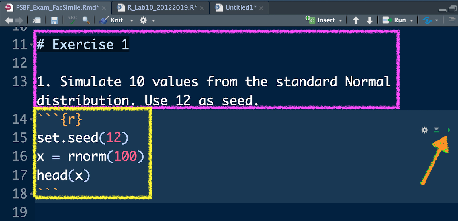
Figure 10.2: Text of an exercise in RMarkdown and code chunk
10.2 Preliminaries on multiple linear regrssion
We introduce the multiple linear regression model, given by the following equation: \[ Y = \beta_0+\beta_1 X_1 +\beta_2X_2+\ldots+\beta_pX_p+ \epsilon \] where \(\beta_0\) is the intercept and \(\beta_j\) is the coefficient of regressor \(X_j\) (\(j=1,\ldots,p\)). The term \(\epsilon\) represents the error with mean equal to zero and variance \(\sigma^2_\epsilon\).
We will use the same data of Lab 7 (file datareg_logreturns.csv) and regarding the daily log-returns (i.e. relative changes) of:
- the NASDAQ index
- ibm, lenovo, apple, amazon, yahoo
- gold
- the SP500 index
- the CBOE treasury note Interest Rate (10 Year)
We start with data import and structure check:
data_logreturns = read.csv("files/datareg_logreturns.csv", sep=";")
str(data_logreturns)
## 'data.frame': 1258 obs. of 10 variables:
## $ Date : chr "27/10/2011" "28/10/2011" "31/10/2011" "01/11/2011" ...
## $ ibm : num 0.02126 0.00841 -0.01516 -0.01792 0.01407 ...
## $ lenovo: num -0.00698 -0.02268 -0.04022 -0.00374 0.07641 ...
## $ apple : num 0.010158 0.000642 -0.00042 -0.020642 0.002267 ...
## $ amazon: num 0.04137 0.04972 -0.01769 -0.00663 0.01646 ...
## $ yahoo : num 0.02004 -0.00422 -0.05716 -0.04646 0.01132 ...
## $ nasdaq: num 0.032645 -0.000541 -0.019456 -0.029276 0.012587 ...
## $ gold : num -0.023184 0.006459 0.030717 0.043197 -0.000674 ...
## $ SP : num 0.033717 0.000389 -0.025049 -0.02834 0.015976 ...
## $ rate : num 0.0836 -0.0379 -0.0585 -0.0834 0.0025 ...10.3 Multiple linear regression model
We start by implementing (again) the simple linear regression model already described in Section 9.1.2, which considers nasdq as dependent (response) variable and SP as independent variable.
mod1 = lm(nasdaq ~ SP, data=data_logreturns)
summary(mod1)
##
## Call:
## lm(formula = nasdaq ~ SP, data = data_logreturns)
##
## Residuals:
## Min 1Q Median 3Q Max
## -0.0128494 -0.0018423 0.0002159 0.0020178 0.0115080
##
## Coefficients:
## Estimate Std. Error t value Pr(>|t|)
## (Intercept) 7.443e-05 8.777e-05 0.848 0.397
## SP 1.085e+00 1.019e-02 106.471 <2e-16 ***
## ---
## Signif. codes: 0 '***' 0.001 '**' 0.01 '*' 0.05 '.' 0.1 ' ' 1
##
## Residual standard error: 0.003109 on 1256 degrees of freedom
## Multiple R-squared: 0.9003, Adjusted R-squared: 0.9002
## F-statistic: 1.134e+04 on 1 and 1256 DF, p-value: < 2.2e-16anova(mod1)## Analysis of Variance Table
##
## Response: nasdaq
## Df Sum Sq Mean Sq F value Pr(>F)
## SP 1 0.109579 0.10958 11336 < 2.2e-16 ***
## Residuals 1256 0.012141 0.00001
## ---
## Signif. codes: 0 '***' 0.001 '**' 0.01 '*' 0.05 '.' 0.1 ' ' 1We implement now the full model by including all the available \(p=8\) regressors. In the R function lm the regressors are specified by name and separated by +:
mod2 = lm(nasdaq ~ ibm + lenovo + apple + amazon + yahoo + gold + SP + rate,
          data= data_logreturns)
summary(mod2)
##
## Call:
## lm(formula = nasdaq ~ ibm + lenovo + apple + amazon + yahoo +
## gold + SP + rate, data = data_logreturns)
##
## Residuals:
## Min 1Q Median 3Q Max
## -0.011522 -0.001574 0.000089 0.001626 0.010487
##
## Coefficients:
## Estimate Std. Error t value Pr(>|t|)
## (Intercept) 6.097e-06 7.208e-05 0.085 0.9326
## ibm -9.625e-03 7.666e-03 -1.256 0.2095
## lenovo 5.123e-03 3.361e-03 1.524 0.1277
## apple 9.209e-02 5.008e-03 18.389 <2e-16 ***
## amazon 5.706e-02 4.285e-03 13.316 <2e-16 ***
## yahoo 3.901e-02 4.681e-03 8.333 <2e-16 ***
## gold -5.936e-03 2.931e-03 -2.025 0.0431 *
## SP 8.884e-01 1.462e-02 60.762 <2e-16 ***
## rate 2.604e-03 3.471e-03 0.750 0.4532
## ---
## Signif. codes: 0 '***' 0.001 '**' 0.01 '*' 0.05 '.' 0.1 ' ' 1
##
## Residual standard error: 0.002547 on 1249 degrees of freedom
## Multiple R-squared: 0.9334, Adjusted R-squared: 0.933
## F-statistic: 2189 on 8 and 1249 DF, p-value: < 2.2e-16In the summary table we have the parameter estimates (\(\hat \beta_0,\hat \beta_1,\ldots,\hat\beta_p\) and \(\sigma_\epsilon=\sqrt{\frac{SSE}{n-1-p}}\)) with the corresponding standard errors (i.e. estimate precision). By means of the t value and the corresponding p-value we can test the hypotheses \(H_0:\beta_j=0\) vs \(H_1:\beta_j\neq 0\) separately for each covariate coefficient (then \(j=1,\ldots,p\)). In the considered case we do not reject the \(H_0\) hypothesis for the following regressors: ibm, lenovo, rate (i.e. the corresponding parameters can be considered null and there is no evidence of a linear relationship). Note that for gold there is a weak evidence from the data against \(H_0\).
Which is the interpretation of the generic \(\hat\beta_j\)? For apple for example the interpretation is the following: when the apple log-return change by one unit, we expect the nasdaq log return to increase by 0.0920924 (when all other covariates are held fixed).
10.3.1 Analysis of variance (sequential and global F tests)
We now apply the function anova to the multiple regression model. This provides us with sequential tests on the single regressors (which are entered one at a time in a hierarchical fashion) and it is useful to assess the effect of adding a new predictor in a given order.
anova(mod2)## Analysis of Variance Table
##
## Response: nasdaq
## Df Sum Sq Mean Sq F value Pr(>F)
## ibm 1 0.040144 0.040144 6186.8396 <2e-16 ***
## lenovo 1 0.006941 0.006941 1069.7375 <2e-16 ***
## apple 1 0.020520 0.020520 3162.4311 <2e-16 ***
## amazon 1 0.013850 0.013850 2134.4469 <2e-16 ***
## yahoo 1 0.006197 0.006197 955.0328 <2e-16 ***
## gold 1 0.000006 0.000006 0.8585 0.3543
## SP 1 0.025956 0.025956 4000.1962 <2e-16 ***
## rate 1 0.000004 0.000004 0.5629 0.4532
## Residuals 1249 0.008104 0.000006
## ---
## Signif. codes: 0 '***' 0.001 '**' 0.01 '*' 0.05 '.' 0.1 ' ' 1In the anova table 0.0081042 is the value of SSE (note that it is lower than the corresponding value observed for mod1).
As shown also in Figure 10.3 and 10.4, the SS values reported in column Sum Sq should be read as the increase in \(SS_R\) when a new variable is added to the predictors already in the model. It’s important to point out that the order of the regressors (used in the lm formula) is relevant and has an effect on the output of the anova function.
The value 0.0401439 represents the additional SSR of the model \(Y=\beta_0+\beta_1 ibm+\epsilon\) with respect to the model with no regressors
\(Y=\beta_0+\epsilon\) (for the latter SSR=0). Note that the two models differs just in one predictor (that’s why df=1). Analyzing the corresponding F-statistic value (with 1 and 1249 degrees of freedom) and p-value, we conclude that the coefficient of ibm is significantly different from zero (and thus ibm is an useful predictor). Similarly, the value 0.0069411 represents the additional SSR of the model \(Y=\beta_0+\beta_1 ibm+\beta_2 lenovo + \epsilon\) with respect to the model containing only ibm: \(Y=\beta_0+\beta_1 ibm+\epsilon\). Also in this case the p-value leads to conclude that lenovo is an useful covariate. This reasoning can be repeated step by step for all the regressors. At the end by summing all the sequential additional SSRs we obtain the total SSR for the model with \(p=8\) regressors:
mod2_an = anova(mod2)
SSR = sum(mod2_an$`Sum Sq`[1:8])
SSR
## [1] 0.1136159The values of SSE instead is contained in the last line of the anova tables under the name Residuals:
SSE = mod2_an$`Sum Sq`[9]
SSE
## [1] 0.008104249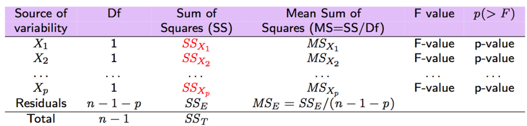
Figure 10.3: Sequential F-tests in case of multiple regression
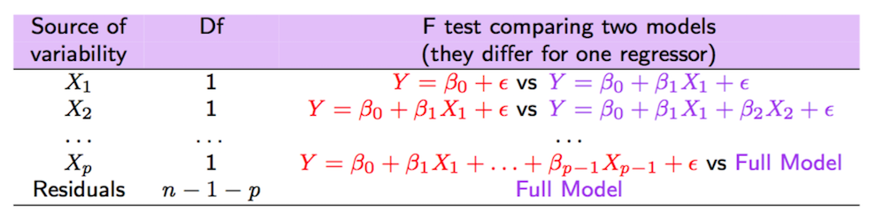
Figure 10.4: Sequential F-tests in case of multiple regression
The values of SSR and SSE can then be used for the global F-test also reported in the last of the summary output. The considered hypotheses are: \(H_0: \beta_1=\beta_2=\ldots=\beta_p=0\) (this corresponds to the model \(Y=\beta_0+\epsilon\)) vs \(H_1: \text{at least one } \beta\neq 0\). As reported in Figure 10.5, the corresponding F-statistic is given by
\[
\text{F-value}=\frac{SS_R/p}{SS_E/(n-1-p)}=\frac{MS_R}{MS_E}
\]
which is a value of the F distribution with \(p\) and \(n-1-p\) degrees of freedom.
If we reject \(H_0\) it means that at least one of the covariates has predictive power in our linear model, i.e. that using a regression is predictively better than
just using the average \(\bar y\) (this is the best prediction in the case of the trivial model with no regressors, \(Y=\beta_0+\epsilon\)).
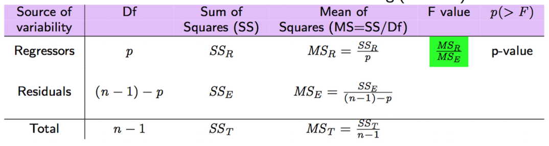
Figure 10.5: Global F-tests for the multiple regression model.
The p-value of this test is reported in the last line of the summary output. (## F-statistic: 2189 on 8 and 1249 DF, p-value: < 2.2e-16). As expected, the p-values is very small and there is evidence for rejecting \(H_0\).
10.3.2 Adjusted \(R^2\)
By using SSR, SSE, SST and the corresponding degrees of freedom (see Figure 10.5), it is possible to compute the adjusted \(R^2\) goodness of fit index: \[ adjR^2 =1- \frac{\frac{SS_E}{n-1-p}}{\frac{SS_T}{n-1}}=1-\frac{MS_E}{MS_T} \] As in the formula of \(adjR^2\) we consider \(p\), there is a penalization for the number of regressors. Thus, \(adjR^2\), differently from the standard \(R^2\) introduced in Section 9.1.3, can increase or decrease. In particular, it increases only when the added variables decrease the SSE enough to compensate for the increase in \(p\).
It can be computed manually as follows:
p = 8
n = nrow(data_logreturns)
SST = sum((data_logreturns$nasdaq - mean(data_logreturns$nasdaq))^2)
1 - (SSE/(n-1-p))/(SST/(n-1))
## [1] 0.9329925but it is also reported in the summary output: Adjusted R-squared: 0.933. This value denotes a very high goodness of fit.
10.3.3 Remove non significant regressors one by one
From the t tests reported in the summary output of mod2, we observed that some of the regressors are not significant. For this reason we remove them one by one, starting from the one with the highest p-value (rate). The following is the new model:
mod3 = lm(nasdaq ~ ibm + lenovo + apple + amazon + yahoo + gold + SP, data= data_logreturns)
summary(mod3)
##
## Call:
## lm(formula = nasdaq ~ ibm + lenovo + apple + amazon + yahoo +
## gold + SP, data = data_logreturns)
##
## Residuals:
## Min 1Q Median 3Q Max
## -0.0114711 -0.0015527 0.0000856 0.0016361 0.0104669
##
## Coefficients:
## Estimate Std. Error t value Pr(>|t|)
## (Intercept) 4.496e-06 7.204e-05 0.062 0.9502
## ibm -9.537e-03 7.664e-03 -1.244 0.2136
## lenovo 5.244e-03 3.357e-03 1.562 0.1185
## apple 9.211e-02 5.007e-03 18.396 <2e-16 ***
## amazon 5.692e-02 4.280e-03 13.298 <2e-16 ***
## yahoo 3.906e-02 4.680e-03 8.346 <2e-16 ***
## gold -6.045e-03 2.927e-03 -2.066 0.0391 *
## SP 8.913e-01 1.409e-02 63.258 <2e-16 ***
## ---
## Signif. codes: 0 '***' 0.001 '**' 0.01 '*' 0.05 '.' 0.1 ' ' 1
##
## Residual standard error: 0.002547 on 1250 degrees of freedom
## Multiple R-squared: 0.9334, Adjusted R-squared: 0.933
## F-statistic: 2502 on 7 and 1250 DF, p-value: < 2.2e-16We note that \(R^2_{adj}\) doesn’t change (thus including rate doesn’t decrease the SSE significantly). We go on by removing ibm which still has a high p-value:
mod4 = lm(nasdaq ~  lenovo + apple + amazon + yahoo + gold + SP, data= data_logreturns)
summary(mod4)
##
## Call:
## lm(formula = nasdaq ~ lenovo + apple + amazon + yahoo + gold +
## SP, data = data_logreturns)
##
## Residuals:
## Min 1Q Median 3Q Max
## -0.0111649 -0.0015513 0.0000687 0.0016327 0.0108501
##
## Coefficients:
## Estimate Std. Error t value Pr(>|t|)
## (Intercept) 8.350e-06 7.199e-05 0.116 0.9077
## lenovo 5.410e-03 3.355e-03 1.612 0.1071
## apple 9.214e-02 5.008e-03 18.398 <2e-16 ***
## amazon 5.711e-02 4.278e-03 13.349 <2e-16 ***
## yahoo 3.941e-02 4.672e-03 8.435 <2e-16 ***
## gold -5.886e-03 2.925e-03 -2.013 0.0444 *
## SP 8.823e-01 1.208e-02 73.027 <2e-16 ***
## ---
## Signif. codes: 0 '***' 0.001 '**' 0.01 '*' 0.05 '.' 0.1 ' ' 1
##
## Residual standard error: 0.002547 on 1251 degrees of freedom
## Multiple R-squared: 0.9333, Adjusted R-squared: 0.933
## F-statistic: 2918 on 6 and 1251 DF, p-value: < 2.2e-16We note that \(R^2_{adj}\) doesn’t change. We go on by removing lenovo:
mod5 = lm(nasdaq ~  apple + amazon +
 yahoo + gold + SP, data= data_logreturns)
summary(mod5)
##
## Call:
## lm(formula = nasdaq ~ apple + amazon + yahoo + gold + SP, data = data_logreturns)
##
## Residuals:
## Min 1Q Median 3Q Max
## -0.0114026 -0.0015730 0.0000785 0.0016151 0.0107557
##
## Coefficients:
## Estimate Std. Error t value Pr(>|t|)
## (Intercept) 6.403e-06 7.202e-05 0.089 0.929
## apple 9.191e-02 5.009e-03 18.348 <2e-16 ***
## amazon 5.702e-02 4.281e-03 13.321 <2e-16 ***
## yahoo 3.987e-02 4.666e-03 8.545 <2e-16 ***
## gold -5.763e-03 2.925e-03 -1.970 0.049 *
## SP 8.871e-01 1.171e-02 75.727 <2e-16 ***
## ---
## Signif. codes: 0 '***' 0.001 '**' 0.01 '*' 0.05 '.' 0.1 ' ' 1
##
## Residual standard error: 0.002549 on 1252 degrees of freedom
## Multiple R-squared: 0.9332, Adjusted R-squared: 0.9329
## F-statistic: 3496 on 5 and 1252 DF, p-value: < 2.2e-16The p-value of gold is very close to alpha=0.05. This is a weak evidence against the hypothesis \(H0:\beta_{gold}=0\). We try to remove also gold and see what happens:
mod6 = lm(nasdaq ~  apple + amazon +
yahoo  + SP, data= data_logreturns)
summary(mod6)
##
## Call:
## lm(formula = nasdaq ~ apple + amazon + yahoo + SP, data = data_logreturns)
##
## Residuals:
## Min 1Q Median 3Q Max
## -0.0114132 -0.0015924 0.0000558 0.0016247 0.0106998
##
## Coefficients:
## Estimate Std. Error t value Pr(>|t|)
## (Intercept) 7.367e-06 7.211e-05 0.102 0.919
## apple 9.186e-02 5.015e-03 18.318 <2e-16 ***
## amazon 5.731e-02 4.283e-03 13.380 <2e-16 ***
## yahoo 3.964e-02 4.670e-03 8.489 <2e-16 ***
## SP 8.871e-01 1.173e-02 75.638 <2e-16 ***
## ---
## Signif. codes: 0 '***' 0.001 '**' 0.01 '*' 0.05 '.' 0.1 ' ' 1
##
## Residual standard error: 0.002552 on 1253 degrees of freedom
## Multiple R-squared: 0.933, Adjusted R-squared: 0.9327
## F-statistic: 4359 on 4 and 1253 DF, p-value: < 2.2e-16We observe that \(R^2_{adj}\) of mod6 is very similar to the one of mod5 (and it’s still a very high goodness of fit!) but mod6 is more parsimonious because it has one parameter less (it’s less complex). For this reason mod6 should be preferred.
10.3.4 AIC computation
To compare models it is also possible to use the Akaike Information Criterion (AIC) given, in the case of multiple regression model, by \[ \text{AIC}=c + n \log({\hat\sigma^2_\epsilon})+2(1+p). \] where \(c\) is a constant not important for model comparison. The criterion for AIC is : the lower, the better.
It is possible to compute the AIC by using the extractAIC function:
extractAIC(mod5)## [1] 6.00 -15019.69extractAIC(mod6)## [1] 5.0 -15017.8The function returns a vector of length 2: the first element represents the total number of parameters (\(p\) + 1 (intercept)), while the second elements is the AIC value. In this case the AIC is lower for mod5; indeed the two AIC values are very similar. For this reason, considering also what it was said in the previous Section, we still prefer mod6 because it has a very high goodness of fit but it’s less complex.
10.4 An authomatic procedure
As an alternative we can use the step() that implement a sequential procedure to find an optimal (actually it is sub-optimal model)
mod_step<- step(mod2)## Start: AIC=-15018.43
## nasdaq ~ ibm + lenovo + apple + amazon + yahoo + gold + SP +
## rate
##
## Df Sum of Sq RSS AIC
## - rate 1 0.0000037 0.008108 -15020
## - ibm 1 0.0000102 0.008114 -15019
## <none> 0.008104 -15018
## - lenovo 1 0.0000151 0.008119 -15018
## - gold 1 0.0000266 0.008131 -15016
## - yahoo 1 0.0004506 0.008555 -14952
## - amazon 1 0.0011505 0.009255 -14853
## - apple 1 0.0021942 0.010298 -14719
## - SP 1 0.0239564 0.032061 -13290
##
## Step: AIC=-15019.86
## nasdaq ~ ibm + lenovo + apple + amazon + yahoo + gold + SP
##
## Df Sum of Sq RSS AIC
## - ibm 1 0.0000100 0.008118 -15020
## <none> 0.008108 -15020
## - lenovo 1 0.0000158 0.008124 -15019
## - gold 1 0.0000277 0.008136 -15018
## - yahoo 1 0.0004518 0.008560 -14954
## - amazon 1 0.0011470 0.009255 -14855
## - apple 1 0.0021951 0.010303 -14720
## - SP 1 0.0259556 0.034064 -13216
##
## Step: AIC=-15020.3
## nasdaq ~ lenovo + apple + amazon + yahoo + gold + SP
##
## Df Sum of Sq RSS AIC
## <none> 0.008118 -15020
## - lenovo 1 0.000017 0.008135 -15020
## - gold 1 0.000026 0.008144 -15018
## - yahoo 1 0.000462 0.008580 -14953
## - amazon 1 0.001156 0.009274 -14855
## - apple 1 0.002196 0.010314 -14721
## - SP 1 0.034606 0.042724 -12933summary(mod_step)##
## Call:
## lm(formula = nasdaq ~ lenovo + apple + amazon + yahoo + gold +
## SP, data = data_logreturns)
##
## Residuals:
## Min 1Q Median 3Q Max
## -0.0111649 -0.0015513 0.0000687 0.0016327 0.0108501
##
## Coefficients:
## Estimate Std. Error t value Pr(>|t|)
## (Intercept) 8.350e-06 7.199e-05 0.116 0.9077
## lenovo 5.410e-03 3.355e-03 1.612 0.1071
## apple 9.214e-02 5.008e-03 18.398 <2e-16 ***
## amazon 5.711e-02 4.278e-03 13.349 <2e-16 ***
## yahoo 3.941e-02 4.672e-03 8.435 <2e-16 ***
## gold -5.886e-03 2.925e-03 -2.013 0.0444 *
## SP 8.823e-01 1.208e-02 73.027 <2e-16 ***
## ---
## Signif. codes: 0 '***' 0.001 '**' 0.01 '*' 0.05 '.' 0.1 ' ' 1
##
## Residual standard error: 0.002547 on 1251 degrees of freedom
## Multiple R-squared: 0.9333, Adjusted R-squared: 0.933
## F-statistic: 2918 on 6 and 1251 DF, p-value: < 2.2e-16we can compare the AIC index between model 6 and the model identified by the step function
extractAIC(mod_step)## [1] 7.0 -15020.3extractAIC(mod6)## [1] 5.0 -15017.8As expected model 6 expresses an higher value of the AIC, nevertheless we still decide to consider this model, having in mind the considerations we have made above.
10.4.1 Plot of observed and predicted values
In the case of multiple regression model it is not possible to plot the estimated regression model, as we did for the simple regression model in Section 9.1.2. This is because it’s a multivariate hyperplane which can not be represented in a 2-D plot. However we can plot together the observed (\(y\)) and predicted values (\(\hat y\), also known as fitted values) of the response variable to have an idea of how good the model is in prediction:
plot(data_logreturns$nasdaq,mod6$fitted.values)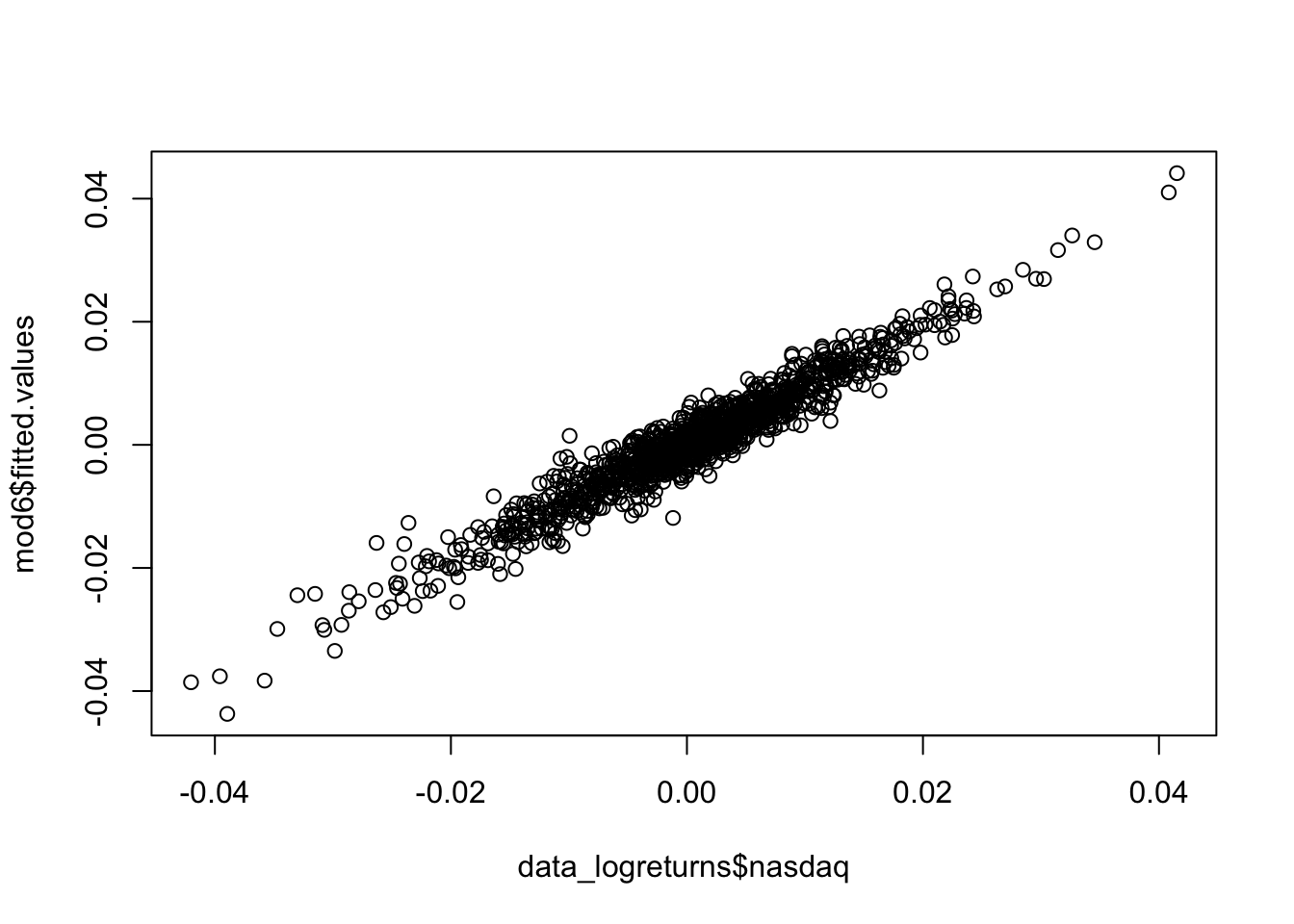
The cloud of points is thin and narrow and this is a sign of a strong linear relationship (correlation is equal to 0.9658989) and a good performance of the model.
10.5 Variance Inflation Factor
The variance inflation factor (VIF) tells how much the variance of \(\hat \beta_j\) for a given regressor \(X_j\) is increased by having other predictors in the model (\(j=1,\ldots,p\)). It is given by \[ VIF_j = \frac{1}{1-R^2_j}\geq 1 \] where \(R^2_j\) is the goodness of fit index for the model which has \(X_j\) has dependent variable and the other remaining regressors as independent variables.
Note that \(VIF_j\) doesn’t provide any information about the relationship between the response and \(X_j\). Rather, it tells us only how correlated \(X_j\) is with the other predictors. We want VIF to be close to one (the latter is the value of VIF when all the regressors are independent).
In R VIF can by computed by using the vif function contained in the faraway library:
library(faraway)
vif(mod6)
## apple amazon yahoo SP
## 1.335137 1.370225 1.381315 1.967353All the four values (one for each regressor in the model) are close to one, so we can conclude that there are no problems of collinearity. A standard threshold for identifying problematic collinearity situation is the value of 5 (or 10).
10.6 Exercise Lab 8
10.6.1 Exercise 1
A linear regression model with three predictor variables was fit to a dataset with 40 observations. The correlation between the observed data \(y\) and the predicted values \(\hat y\) is 0.65. The total sum of squares (SST) is 100.
What is the value of the non-adjusted goodness of fit index (\(R^2\))? You have to think of an alternative way to compute \(R^2\)… see theory lectures. Comment the value.
What is the value of the residual sum of squares (SSE)?
What is the value of the regression sum of squares (SSR)?
What is the estimate of \({\sigma^2_\epsilon}\)?
Fill in the following ANOVA table. To compute the p-value associated to the F-value of the F statistic you have to use the
pffunction (see?pf):
| Source of variability | Df | Sum of Squares (SS) | Mean Sum of Squares (MS) | F value | p(>F) |
|---|---|---|---|---|---|
| Regressors | … | … | … | … | … |
| Residuals | … | … | … | ||
| Total | … | … |
- What do you think about the fitted model?
10.6.2 Exercise 2
- Complete the following ANOVA table for the linear regression model \(Y=\beta_0+\beta_1X_1+\beta_2X_2+\epsilon\). Explain all the steps of your computations. Suggestion: start with the degrees of freedom and then the p-value. To obtain the F-value given the p-value you will need the
qffunction (see?qf).
| Source of variability | Df | Sum of Squares (SS) | Mean Sum of Squares (MS) | F value | p(>F) |
|---|---|---|---|---|---|
| Regressors | … | … | … | … | 0.04 |
| Residuals | … | 5.66 | … | ||
| Total | 15 | … |
What do you think about the fitted model?
Determine the value of \(R^2\) and of the adjusted \(R^2\). Comment.
10.6.3 Exercise 3
Use again the data in the prices_5Y.csv file alty used for Lab 7. They refer to daily prices (Adj.Close) for the period 05/11/2012-03/11/2017 for the following assets: Apple (AAPL), Intel (INTC), Microsoft (MSFT) and Google (GOOGL). Import the data in R.
Create a new data frame containing the log returns for all the assets.
Estimate the parameters of the multiple linear model which considers
GOOGLas dependent variable and includes all the remaining explanatory variables. Are all the coefficients significantly different from zero? Comment the results.Do you suggest to remove some of the regressors?
Comment about the goodness of fit of the model.
Comment the
anovatable for the multiple linear regression model. Moreover, derive from the table the values of SSR, SSE and SST.Compute manually the value of the F-statistic reported in the last line of the
summaryoutput. Compute also the corresponding p-value and comment the result.Plot the observed and predicted values of the response variable.