Chapter 9 Lab 7 - 26/11/2021
In this lecture we will will introduce the simple linear regression model.
We will use the data stored in the datareg_logreturns.csv file regarding the daily log-returns (i.e. relative changes) of:
- the NASDAQ index
- ibm, lenovo, apple, amazon, yahoo
- gold
- the SP500 index
- the CBOE treasury note Interest Rate (10 Year)
We consider as response variable (dependent variable) the log-returns of the NASDAQ index. All the others are independent variables (asa regressors, covariates or features).
We start with data import and its structure check:
datareg = read.csv("files/datareg_logreturns.csv", sep=";")
str(datareg)
## 'data.frame': 1258 obs. of 10 variables:
## $ Date : chr "27/10/2011" "28/10/2011" "31/10/2011" "01/11/2011" ...
## $ ibm : num 0.02126 0.00841 -0.01516 -0.01792 0.01407 ...
## $ lenovo: num -0.00698 -0.02268 -0.04022 -0.00374 0.07641 ...
## $ apple : num 0.010158 0.000642 -0.00042 -0.020642 0.002267 ...
## $ amazon: num 0.04137 0.04972 -0.01769 -0.00663 0.01646 ...
## $ yahoo : num 0.02004 -0.00422 -0.05716 -0.04646 0.01132 ...
## $ nasdaq: num 0.032645 -0.000541 -0.019456 -0.029276 0.012587 ...
## $ gold : num -0.023184 0.006459 0.030717 0.043197 -0.000674 ...
## $ SP : num 0.033717 0.000389 -0.025049 -0.02834 0.015976 ...
## $ rate : num 0.0836 -0.0379 -0.0585 -0.0834 0.0025 ...9.1 Simple linear regression model
9.1.1 Covariance and correlation
The linear relationship existing between two quantitative variables can by studied by using the scatterplot or by means of the covariance and correlation index. For example the following code produce the scatterplot between a couple of variables (ibm - independent variable - and nasdaq - dependent variable):
plot(datareg$ibm, datareg$nasdaq)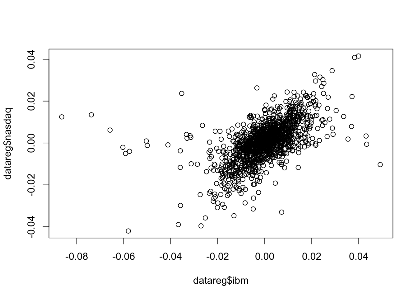
It is clear that a positive relationship exists between the two variables (see the cloud of points with increasing direction). We observe also tail dependence in the plot (high/low values of ibm occur jointly with high/low values of nasdaq). However also some observations connected with tail independence are visible in the plot (see the points corresponding to low negative values of ibm and positive values of nasdaq).
To compute the covariance and correlation index we use the cov and cor functions:
cov(datareg$ibm, datareg$nasdaq) ## [1] 6.783533e-05cor(datareg$ibm, datareg$nasdaq)## [1] 0.5742862We observe that both the indexes are positive, as expected given the shape of the cloud of points. The value 0.57 denotes an average level of linear association.
It is also possible to get the variance-covariance matrix and the correlation matrix with cov(x) and
cor(x), where x is a data frame or a selection of some columns in it. Before proceeding we have to remove the first column containing the dates (we overwrite datareg with a new data frame created started from datareg and by selecting all the columns except the first one):
datareg = datareg[,-1]
cov(datareg) #variance-covariance matrix
## ibm lenovo apple amazon yahoo
## ibm 1.440880e-04 5.018175e-05 6.154061e-05 6.708451e-05 5.879838e-05
## lenovo 5.018175e-05 5.243653e-04 5.723924e-05 7.734088e-05 9.423343e-05
## apple 6.154061e-05 5.723924e-05 2.750300e-04 7.906427e-05 7.324756e-05
## amazon 6.708451e-05 7.734088e-05 7.906427e-05 3.869414e-04 1.287336e-04
## yahoo 5.879838e-05 9.423343e-05 7.324756e-05 1.287336e-04 3.281435e-04
## nasdaq 6.783533e-05 7.653079e-05 9.610814e-05 1.105234e-04 9.789117e-05
## gold -1.043981e-05 1.450081e-05 1.706496e-06 -1.298227e-05 7.818512e-06
## SP 6.406188e-05 6.842926e-05 7.147921e-05 8.565277e-05 7.978556e-05
## rate 7.738766e-05 1.000652e-04 8.378584e-05 8.419878e-05 9.519658e-05
## nasdaq gold SP rate
## ibm 6.783533e-05 -1.043981e-05 6.406188e-05 7.738766e-05
## lenovo 7.653079e-05 1.450081e-05 6.842926e-05 1.000652e-04
## apple 9.610814e-05 1.706496e-06 7.147921e-05 8.378584e-05
## amazon 1.105234e-04 -1.298227e-05 8.565277e-05 8.419878e-05
## yahoo 9.789117e-05 7.818512e-06 7.978556e-05 9.519658e-05
## nasdaq 9.683385e-05 -3.823920e-06 8.037427e-05 9.373488e-05
## gold -3.823920e-06 6.049650e-04 -7.393048e-08 -2.435893e-05
## SP 8.037427e-05 -7.393048e-08 7.410393e-05 8.577946e-05
## rate 9.373488e-05 -2.435893e-05 8.577946e-05 5.306421e-04cor(datareg) #correlation matrix## ibm lenovo apple amazon yahoo nasdaq
## ibm 1.0000000 0.18256390 0.309141875 0.28410946 0.27040797 0.57428618
## lenovo 0.1825639 1.00000000 0.150725539 0.17169970 0.22717272 0.33962969
## apple 0.3091419 0.15072554 1.000000000 0.24236375 0.24382108 0.58892032
## amazon 0.2841095 0.17169970 0.242363747 1.00000000 0.36127453 0.57097612
## yahoo 0.2704080 0.22717272 0.243821083 0.36127453 1.00000000 0.54915892
## nasdaq 0.5742862 0.33962969 0.588920320 0.57097612 0.54915892 1.00000000
## gold -0.0353601 0.02574602 0.004183599 -0.02683262 0.01754798 -0.01579902
## SP 0.6199620 0.34713968 0.500690167 0.50582255 0.51164856 0.94881773
## rate 0.2798703 0.18969900 0.219320776 0.18581568 0.22813327 0.41351071
## gold SP rate
## ibm -0.0353601041 0.6199619759 0.27987034
## lenovo 0.0257460172 0.3471396840 0.18969900
## apple 0.0041835993 0.5006901672 0.21932078
## amazon -0.0268326183 0.5058225541 0.18581568
## yahoo 0.0175479795 0.5116485609 0.22813327
## nasdaq -0.0157990161 0.9488177268 0.41351071
## gold 1.0000000000 -0.0003491707 -0.04299245
## SP -0.0003491707 1.0000000000 0.43257539
## rate -0.0429924489 0.4325753882 1.00000000Note that the correlation matrix is a 9x9 symmetric (so that for example Cor(ibm,nasdaq)=Cor(nasdaq,ibm)) matrix; moreover, all the values in the the diagonal are equal to one.
It is possible to consider also all the possible couples of variable in datareg and get a matrix of scatterplots by using the function pairs(x), where x is a data frame or a selection of some columns in it.
pairs(datareg)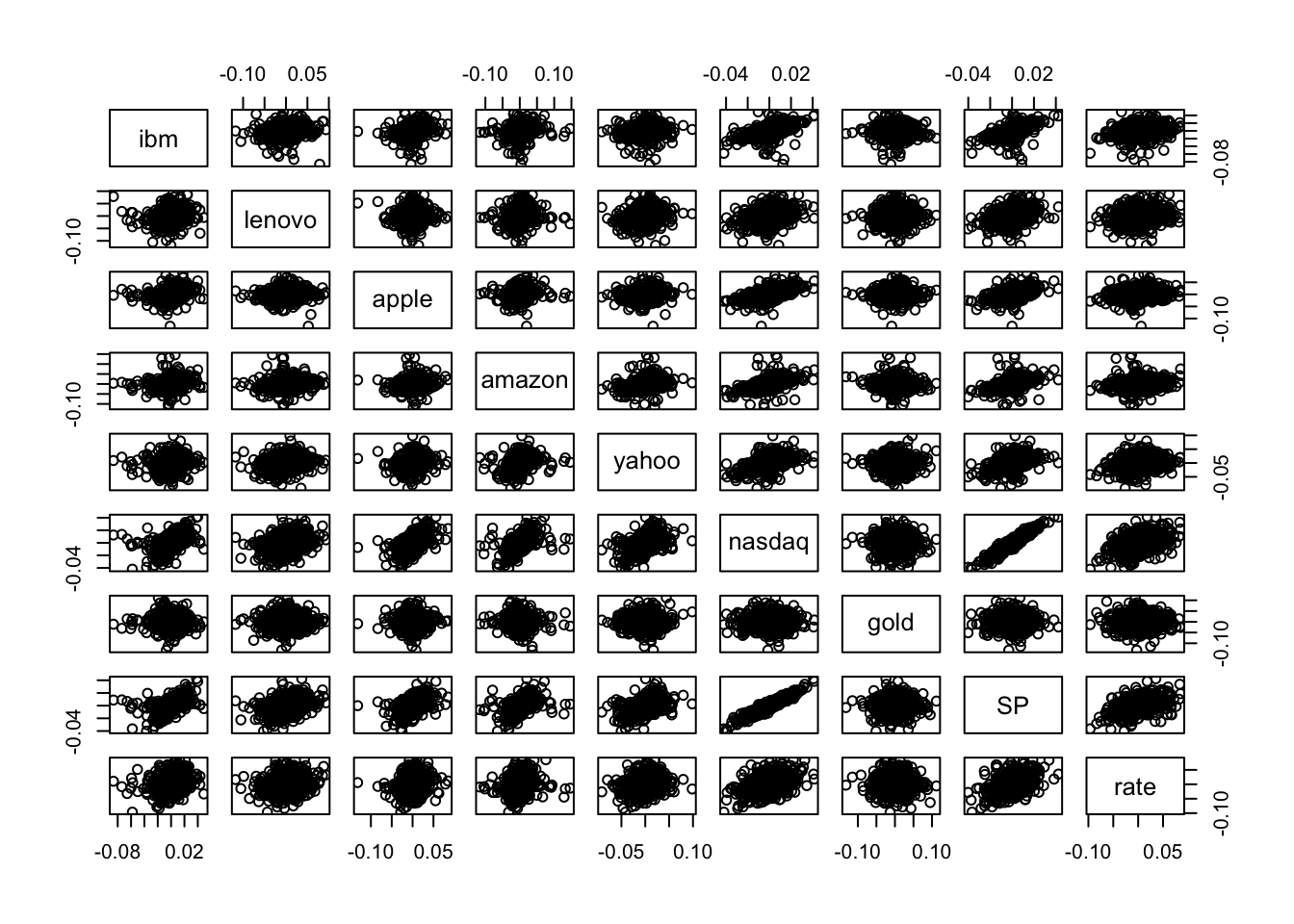 Note that the scatterplot matrix is not symmetric: for example the plot in the second row and first column is not equal to the plot in the first row and second column because the axes are exchanged (in the former lenovo is represented on the y-axis, while in the latter lenovo is on the x-axis).
In the scatterplot matrix just two cases show a thin cloud of points denoting a strong linear relationship: the plots referred to nasdaq and SP. As reported also in the correlation matrix, the correlation between these two variables is very close to one and equal to
cor(datareg$nasdaq,datareg$SP)## [1] 0.9488177Thus, we decide to use SP as regressor in the simple regression model that will be estimated in the following section.
9.1.2 Simple linear regression model
Consider nasdq as dependent (response) variable and SP as independent variable, thus in this case the number of regressor is \(p=1\). The linear model equation is given by
\[
Y = \beta_0+\beta_1 X + \epsilon
\]
where \(\beta_0\) is the intercept and \(\beta_1\) the slope. The term \(\epsilon\) represents the error with mean equal to zero and variance \(\sigma^2_\epsilon\).
The function to be used in R to estimate a linear regression model is lm (linear model):
lm(nameofy ~ nameofx, data=nameofdataframe)The \(\sim\) symbol (tilde) can be obtained by:
- pressing ALT and 5 with Mac
- pressing ALT 1, 2 and 6 with Windows equipped with numeric keypad
- pressing ALT and Fn and 1, 2 and 6 with Windows without numeric keypad
The model we are interested in can be estimated as follows:
mod1 = lm(nasdaq ~ SP, data=datareg)The object mod1 is a list containing 12 the following 12 elements:
names(mod1)## [1] "coefficients" "residuals" "effects" "rank"
## [5] "fitted.values" "assign" "qr" "df.residual"
## [9] "xlevels" "call" "terms" "model"In particular we are interested in:
- the least squares estimates \(\hat\beta_0\) and \(\hat \beta_1\):
mod1$coefficients## (Intercept) SP
## 7.443203e-05 1.084615e+00The slope estimate (1.085) suggests that when the SP log-return increases by one unit we expect an increase of 1.085 in the nasdaq log-return. The estimated model \(\hat y=\hat\beta_0+\hat\beta_1 x\) is given by the following straight line included in the scatterplot:
plot(datareg$SP, datareg$nasdaq)
abline(mod1,col="red",lwd=2)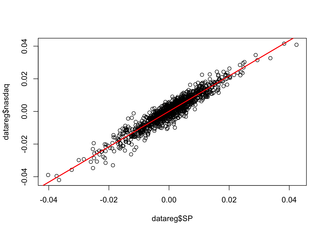
- the fitted values given by \(\hat y_i=\hat\beta_0+\hat\beta_1 x_i\) (\(i=1,\ldots,n\) with $n=$1258).
head(mod1$fitted.values)## 1 2 3 4 5
## 0.0366439651 0.0004965144 -0.0270936832 -0.0306636329 0.0174026410
## 6
## 0.0202565287- the residuals given by the difference between observed and fitted values: \(y_i -\hat y_i\) (\(i=1,\ldots,n\) with $n=$1258).
head(mod1$residuals)## 1 2 3 4 5 6
## -0.003998621 -0.001037069 0.007637417 0.001387478 -0.004816084 0.001471765All the important information related to the estimated model can be obtained by using the summary function:
summary(mod1)##
## Call:
## lm(formula = nasdaq ~ SP, data = datareg)
##
## Residuals:
## Min 1Q Median 3Q Max
## -0.0128494 -0.0018423 0.0002159 0.0020178 0.0115080
##
## Coefficients:
## Estimate Std. Error t value Pr(>|t|)
## (Intercept) 7.443e-05 8.777e-05 0.848 0.397
## SP 1.085e+00 1.019e-02 106.471 <2e-16 ***
## ---
## Signif. codes: 0 '***' 0.001 '**' 0.01 '*' 0.05 '.' 0.1 ' ' 1
##
## Residual standard error: 0.003109 on 1256 degrees of freedom
## Multiple R-squared: 0.9003, Adjusted R-squared: 0.9002
## F-statistic: 1.134e+04 on 1 and 1256 DF, p-value: < 2.2e-16In the central part of the summary table (named Coefficients) the following information are reported:
Estimate(\(\hat \beta_0\) denoted by(Intercept)and \(\hat \beta_1\) denoted bySP);Std.Error: the estimate of the standard deviation of \(\hat\beta_0\) and \(\hat\beta_1\) (this is a measure of the precision of the estimates; the lower the better);t.value: this is t test statistic given by the ratio betweenEstimateandStd.Errorand it’s a realization of a Student t distribution with \(n-p-1\)=nrow(datareg)-2degrees of freedom;Pr(>|t|): this is the corresponding p-value connected with the t test statistic.
In the considered case we reject the hypothesis \(H_0:\beta_1=0\) (thus SP is a significant regressor) and do not reject the hypothesis \(H_0:\beta_0=0\) (but in any case we keep the intercept in the model).
9.1.3 Variance decomposition
In the following we introduce some important quantities connected with the decomposition of the deviance of the dependent variable (\(SST=SSR+SSE\), see Figure 9.1).
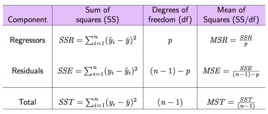
Figure 9.1: Anova table
The total variability of nasdaq is represented by \(SST\) (total sum of squares) which can be computed as follows:
SST = sum((datareg$nasdaq - mean(datareg$nasdaq)) ^2)
SST
## [1] 0.1217202The sum of squares of the errors (SSE) can be obtained by:
SSE = sum(mod1$residuals^2)
SSE
## [1] 0.01214097#SSE = sum((datareg$nasdaq-mod1$fitted.values)^2)Given that \(SST=SSR+SSE\), \(SSR\) can be derived as follows:
SSR = SST-SSE
#SSR=sum((mod1$fitted.values-mean(datareg$nasdaq))^2)
Given these important quantities the goodness of fit index \(R^2\) can be easily derived as the ratio between \(SSR\) and \(SST\):
SSR/SST## [1] 0.90025511-SSE/SST## [1] 0.9002551We obtain that SSR/SST*100 of the total variability of nasdaq is explained by SP. Consider that the range of the \(R^2\) index is the interval \([0,1]\): so, this is a very good performance of the linear model! Note that the \(R^2\) index is also reported in the summary output as Multiple R-squared: 0.9003.
All the important quantities related to the variance decomposition and reported in Figure 9.2 can be obtained also by using the function anova:
anova(mod1)## Analysis of Variance Table
##
## Response: nasdaq
## Df Sum Sq Mean Sq F value Pr(>F)
## SP 1 0.109579 0.10958 11336 < 2.2e-16 ***
## Residuals 1256 0.012141 0.00001
## ---
## Signif. codes: 0 '***' 0.001 '**' 0.01 '*' 0.05 '.' 0.1 ' ' 1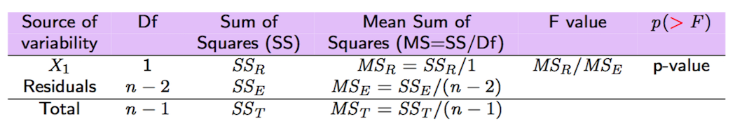
Figure 9.2: Anova table with F-test
9.1.4 F-test
The F-test reported in the anova output considers, in this case with \(p=1\), \(H_0: \beta_1=0\) vs \(H_0: \beta_1\neq 0\); the corresponding test statistic value is given by
\[
\text{F-value}=\frac{SS_R/1}{SS_E/(n-2)}=\frac{MS_R}{MS_E}
\]
which is a value of the F distribution (see here) with 1 and \(n-2\) degrees of freedom. We expect high value of the test statistic if the regressor is highly significant. In the case of simple regression, the F-test leads to the same conclusion of the t-test for \(\beta_1\). So, given the small p-value reported in the anova table we conclude, again, that SP is a significant regressor. Note that the output of the F-test are also reported in the last line of the summary ouptut (F-statistic: 1.134e+04 on 1 and 1256 DF, p-value: < 2.2e-16).
9.1.5 Estimate of the error variance
The estimate of the error variance \(\sigma^2_\epsilon\) is given by \(\hat\sigma^2_\epsilon=\frac{SSE}{n-p-1}\) and can be computed as follows
SSE/(nrow(datareg)-length(mod1$coefficients))## [1] 9.666375e-06The corresponding square root
sqrt(SSE/(nrow(datareg)-2))## [1] 0.003109079is also reported in the summary output as Residual standard error: 0.003109 on 1256 degrees of freedom.
9.2 Exercise Lab 7
9.2.1 Exercise 1
Use the data in the prices_5Y.csv which refer to daily prices (Adj.Close) for the period 05/11/2012-03/11/2017 for the following assets: Apple (AAPL), Intel (INTC), Microsoft (MSFT) and Google (GOOGL). Import the data in R.
Plot the time series of
GOOGL(use dates along the x-axis). Comment the plot.Create a new data frame containing the log returns for all the assets.
Plot the time series of
GOOGLlog-returns (use dates along the x-axis, but pay attention because you will have to remove the first date). Comment the plot.Use the normal probability plot and the Kolmogorov-Smirnov test to study the normality of
GOOGLlog-returns. Comment your results.Consider all the assets. Compute the correlation matrix. Comment the values. Which is the correlation value between
GOOGLandMSFT?Plot all the scatterplots and comment about tail dependence-independence of GOOGL-MSFT.
Estimate the simple linear model which considers
GOOGLas dependent variable andMSFTas independent variable. Provide the summary output and comment the slope estimate.Plot the two considered variables together with the estimated regression line.
Compute the following quantities: SST, SSE, SSR and the \(R^2\) coefficient. Comment the goodness of fit coefficient. Furthermore, check that it corresponds to the one in the
summaryoutput.Check that the goodness of fit index \(R^2\) is also equal to the squared correlation index between fitted and observed values: \(Cor(y,\hat y)^2\).
Check that the goodness of fit index \(R^2\) is also equal to the squared correlation index between
GOOGLandMSFT: \(Cor(x,y)^2\).Compute the estimate of the variance of the errors \(\sigma^2\). Can you find the same value in the
summaryoutput?Create the anova table and comment the F-test p-value (define also the H0 and H1 hypotheses).
In the anova table obtained at the previous point, which values do you have in the
Sum Sqcolumn?Estimate the
GOOGLlog-return value when theMSFTlog-return is equal to 0.0007.