Chapter 6 Lab 4 - 30/10/2021
In this lecture we will estimate the cumulative distribution function (CDF) of a marginal distribution by using the empirical cumulative distribution function (ECDF). Moreover, we will learn how to fit a theoretical distribution (like the normal or t model) to a set of data.
We use the file named prices.csv already introduced for Lab. 3 (see Chapter 5). We start with data import and structure check:
prices <- read.csv("~/Dropbox/UniBg/Didattica/Economia/2021-2022/PSBF_2122/R_LABS/Lab03/prices.csv")
head(prices)
## Date A2Aadj ISPajd JUVEadj
## 1 10/01/17 0.982659 1.597666 0.288256
## 2 11/01/17 0.999368 1.595077 0.289546
## 3 12/01/17 1.012895 1.573067 0.288164
## 4 13/01/17 1.030400 1.596372 0.289546
## 5 16/01/17 1.021647 1.566594 0.284573
## 6 17/01/17 1.022443 1.566594 0.288256str(prices)## 'data.frame': 1213 obs. of 4 variables:
## $ Date : chr "10/01/17" "11/01/17" "12/01/17" "13/01/17" ...
## $ A2Aadj : num 0.983 0.999 1.013 1.03 1.022 ...
## $ ISPajd : num 1.6 1.6 1.57 1.6 1.57 ...
## $ JUVEadj: num 0.288 0.29 0.288 0.29 0.285 ...In particular we focus on the Intesa San Paolo price variable named ISPajd and compute the corresponding log-returns:
logret = diff(log(prices$ISPajd))6.1 Empirical cumulative distribution function
The empirical cumulative distribution function (ECDF) returns the proportion of values in a vector which are lower than or equal to a given real value \(y\). It is defined as \[ F_n(y)=\frac{\sum_{i=1}^n \mathbb I(Y_i\leq y)}{n} \] where \(\mathbb I(\cdot)\) is the indicator function which is equal to one if \(Y_i\leq y\) or 0 otherwise (basically you simply count the number of observations \(\leq y\) over the total number of observations \(n\)).
It can be obtained by saving the output of the ecdf function in an object:
myecdf = ecdf(logret)The object myecdf belongs to the function class and can be used to compute proportions, such as for example the probability of having a value lower than or equal to -0.04:
myecdf(-0.04) ## [1] 0.01732673The output returns the proportion of log-returns lower than or equal to -0.04. It can be interesting to compute the percentage of negative or null log-returns (i.e. losses or no changes):
myecdf(0)*100## [1] 49.75248and the corresponding percentage of positive log-returns (i.e. gains):
1 - myecdf(0)## [1] 0.5024752Note that the input of the myecdf function can be any real number. For the considered example the ecdf is equal to 0 for values lower than the lowest observed value (-0.2) and equal to 1 for values bigger than the largest observed value (0.2). As expected, if we evaluate the ecdf for the median value we get 50% (for the definition of median):
myecdf(median(logret))*100## [1] 50The ecdf can be plotted by using
plot(myecdf)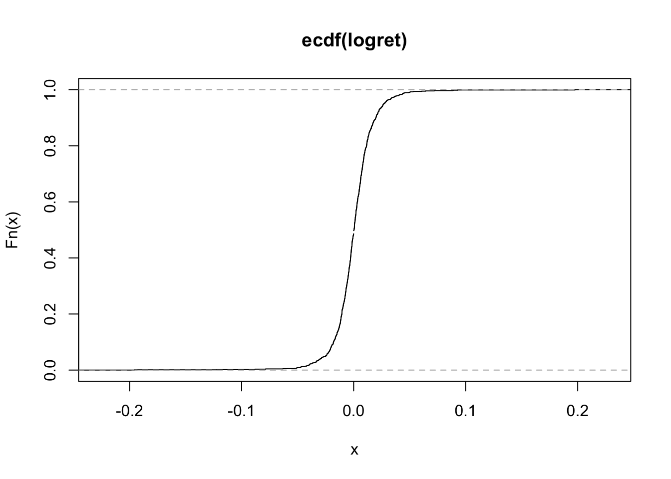 On the x-axis we could have values from \(-\infty\) to \(+\infty\) (but only values between the min and max of the observed values are shown as they are the most interesting). On the y-axis we have the values of the ecdf and so proportions (which are always between 0 and 1).
By looking at the plot it is possible to get, for a particular value on the x-axis, the corresponding ecdf. To have a better view of the ecdf line we zoom the plot for the values of the x-axis between 1.8 and 2.2.
plot(myecdf, xlim = c(-0.001, +0.001))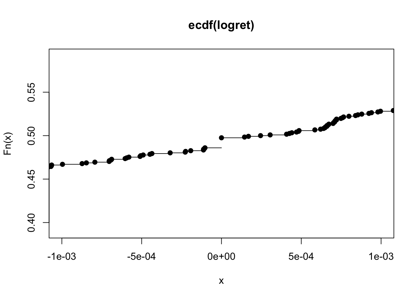 It is evident that the ecdf is defined for all the real values and is a non-decreasing function (it is never decreasing). It is a step function: in particular, steps occur in correspondence with the observed log-return values (and the jump of each step is equal to \(1/n\)). The slope of the ecdf gives important information about the distribution and the variability of the data. In particular, a steeper slope means less variability, while a shallower slope indicates a greater spread in your data.
It is also possible to include in the plot some constant vertical or horizontal lines:
plot(myecdf)
#add a vertical line for x=median
abline(v = median(logret),
       col = "red",
       lty = 2) #line type (dashed)
#corresponding proportion line (0.5)
abline(h = myecdf(median(logret)),
       col = "red",
       lty = 2) #line type (dashed)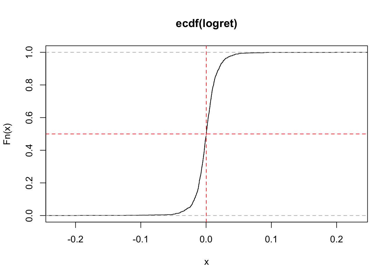
6.2 Fit a distribution to the data
In this Section we learn to fit a distribution, whose probability density function (PDF) is known (e.g. Normal distribution or t distribution), to the data. The parameters of the theoretical model are estimated by using the maximum likelihood (ML) approach. The function in R for this analysis is called fitdistr and it is contained in the MASS library. The latter is already available in the standard release of R and it is not necessary to install it; you just have to load it. The inputs of fitdistr are: the data and the theoretical chosen model (see ?fitdistr for the available options). Let’s consider first the case of the Normal distribution:
library(MASS) #load the library
fitN = fitdistr(logret,densfun="normal")
fitN
## mean sd
## 0.0003584645 0.0191062378
## (0.0005488123) (0.0003880689)The output of fitN provides the ML estimates of the parameters of the Normal distribution (in this case mean \(\mu\) and sd \(\sigma\)) with the corresponding standard errors provided in parentheses (i.e. the standard deviation of the ML estimates) which represent a measure of accuracy of the estimates (the lower the better). In case of Normal model, the ML of the mean \(\mu\) is given by the sample mean \(\bar x=\frac{\sum_{i=1}^n x_i}{n}\), while the ML of the variance is given by the biased sample variance \(s^2 =\frac{\sum_{i=1}^n (x_i-\bar x)^2}{n}\).
Note from the top-right panel that the object fitN is a list (this is a new kind of object for us1) containing 5 elements that can be displayed using
names(fitN)## [1] "estimate" "sd" "vcov" "n" "loglik"To extract one element from a list we use the dollar; for example to extract from fitN the object containing the parameter estimates:
fitN$estimate #vector of estimates## mean sd
## 0.0003584645 0.0191062378fitN$estimate[1] #first estimate## mean
## 0.0003584645fitN$estimate[2] #second estimate## sd
## 0.01910624Another distribution can be fitted to the data, such as for example the (so called standardized) t distribution \(t_\nu^{std}(\mu,\sigma^2)\). Note that in this case three parameters are estimated using the ML approach: mean \(\mu\), sd \(\sigma\) and degrees of freedom \(\nu\) (df):
fitT = fitdistr(logret,"t")## Warning in dt((x - m)/s, df, log = TRUE): NaNs produced## Warning in log(s): NaNs produced
## Warning in log(s): NaNs produced
## Warning in log(s): NaNs produced## Warning in dt((x - m)/s, df, log = TRUE): NaNs produced## Warning in log(s): NaNs produced
## Warning in log(s): NaNs produced

## Warning in log(s): NaNs produced

## Warning in log(s): NaNs produced
## Warning in log(s): NaNs produced
## Warning in log(s): NaNs produced
## Warning in log(s): NaNs produced
## Warning in log(s): NaNs produced
## Warning in log(s): NaNs produced
## Warning in log(s): NaNs produced
## Warning in log(s): NaNs produced
## Warning in log(s): NaNs produced
## Warning in log(s): NaNs produced
## Warning in log(s): NaNs produced
## Warning in log(s): NaNs produced
## Warning in log(s): NaNs produced
## Warning in log(s): NaNs producedfitT## m s df
## 0.0002769408 0.0112523654 2.9995749290
## (0.0003955436) (0.0004137404) (0.2865319395)6.2.1 AIC and BIC
Which is the best model between the Normal and the t distribution? To compare them we can use the log likelihood value of the two fitted model (which is provided as loglik in the output of fitdistr): the higher the better.
fitN$loglik## [1] 3077.028fitT$loglik ## [1] 3293.928In this case the t distribution has a higher log likelihood value. A similar conclusion is obtained by using the deviance which is a misfit index that should be minimized (the smaller the deviance the better the fit): the deviance is given by \[\text{deviance} = -2*\text{loglikelihood}.\]
-2*fitN$loglik## [1] -6154.056-2*fitT$loglik ## [1] -6587.857Again the t distribution performs better in term of goodness of fit but it is also a more complex model (one extra parameter to estimate). Can we consider also model complexity? The Akaike Information Criterion (AIC) and the Bayes information criterion (BIC) indexes take into account model complexity by penalizing for the number of parameters to be estimated: \[ AIC = \text{deviance}+2p \]
\[ BIC = \text{deviance}+\log(n)p \] where \(p\) is the numbers of estimated parameters (2 for the Normal model and 3 for the t distribution) and \(n\) the sample size. The terms \(2p\) and \(\log(n)p\) are called complexity penalties.
Both AIC and BIC follow the criterion smaller is better, since small values of AIC and BIC tend to minimize both the deviance and model complexity. Note that usually \(\log(n)>2\), thus BIC penalizes model complexity more than AIC. For this reason, BIC tends to select simpler models.
#### AIC ####
#AIC for the normal model
-2*fitN$loglik + 2* length(fitN$estimate)
## [1] -6150.056#AIC for the t model
-2*fitT$loglik + 2* length(fitT$estimate)## [1] -6581.857#### BIC ####
#BIC for the normal model
-2*fitN$loglik + log(length(logret)) * length(fitN$estimate)## [1] -6139.856#BIC for the t model
-2*fitT$loglik + log(length(logret)) * length(fitT$estimate)## [1] -6566.557The two indexes can be computed also by using the R functions AIC and BIC:
AIC(fitN)## [1] -6150.056AIC(fitT)## [1] -6581.857BIC(fitN)## [1] -6139.856BIC(fitT)## [1] -6566.557If we compare the AIC and BIC values we prefer the t model, which outperforms the Normal model also when adjusting by model complexity.
6.2.2 Plot of the density function of the Normal distribution
Let’s compare graphically the KDE of logret with the Normal PDF fitted to the data given by the following formula (the parameters \(\mu\) and \(\sigma^2\) are substituted by the corresponding estimates):
\[
\hat f(x)=\frac{1}{\sqrt{2\pi s^2}}e^{-\frac{1}{s^2}(x-\bar x)^2}
\]
To compute the PDF values we use the dnorm(x,mean,sd) function which returns the values of the Normal probability density function evaluated for a set of values x. In this case given the KDE plot
plot(density(logret))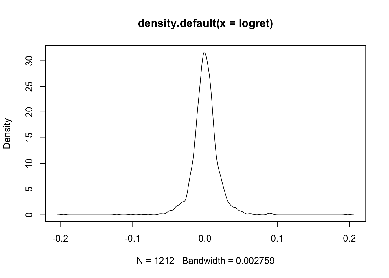 we are interested in evaluating the PDF for the values between -0.2 and +0.2. We thus create a regular sequence of 500 (
length) values from -0.2 to +0.2 by means of the seq function:
xseq = seq(from=-0.2, to=+0.2, length=500)
# have a look to this regular sequence
head(xseq)
## [1] -0.2000000 -0.1991984 -0.1983968 -0.1975952 -0.1967936 -0.1959920tail(xseq)## [1] 0.1959920 0.1967936 0.1975952 0.1983968 0.1991984 0.2000000We are now ready to compute the values of the PDF for all the values in xseq considering a Normal distribution with mean and sd given by fitN$estimates:
densN = dnorm(xseq,
          mean=fitN$estimate[1],
          sd=fitN$estimate[2])
The vector densN contains 1000 values for the Normal PDF. We are now ready to combine in a plot the KDE with the Normal PDF:
plot(density(logret),col="blue")
lines(xseq, densN,col="red")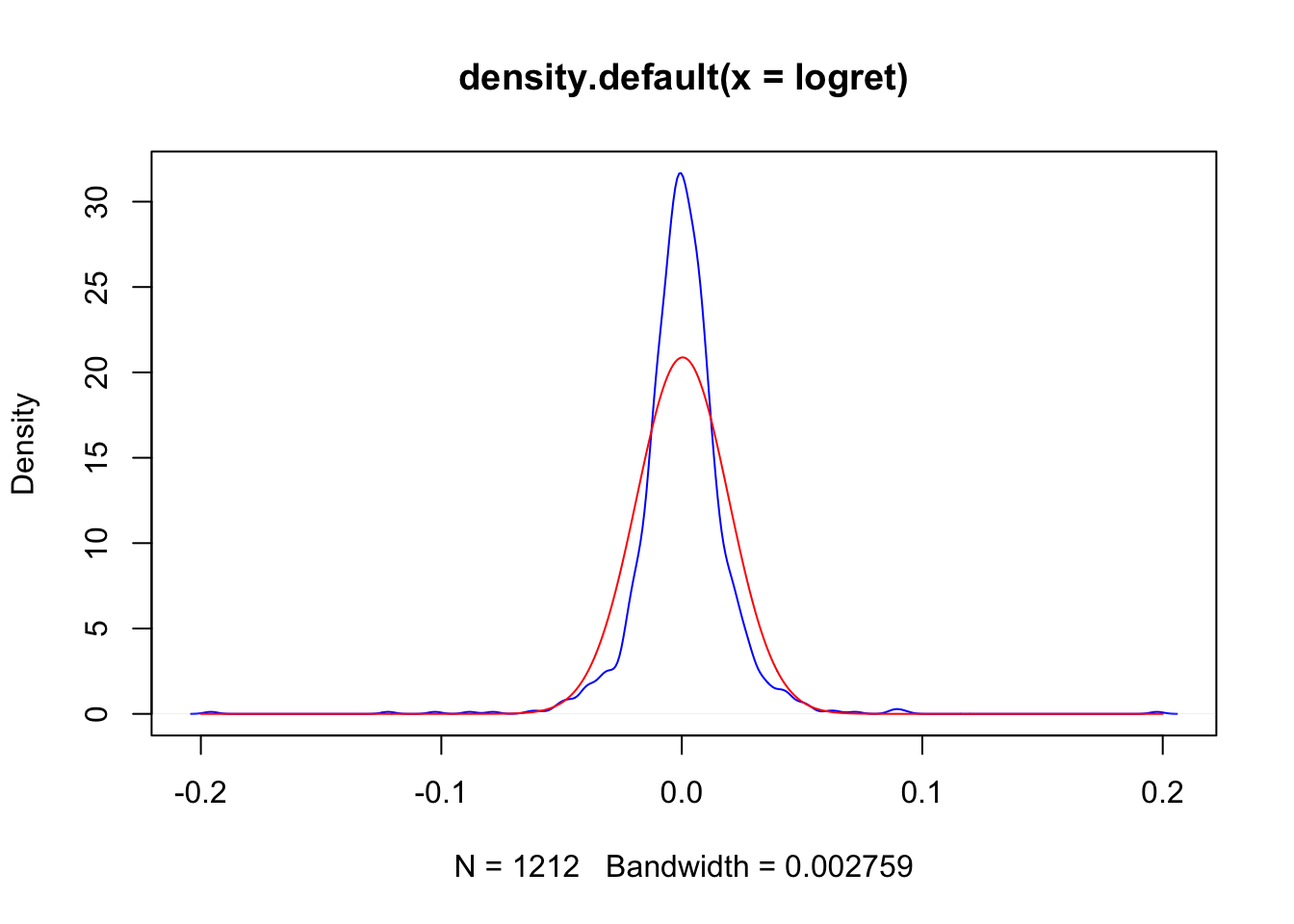
It appears that there are some differences between the (empirical) KDE (blue line) and the Normal (theoretical) PDF (red line).
6.2.3 Plot of the density function of the t distribution
The PDF of the standardized t distribution \(t_\nu^{std}(\mu,\sigma^2)\) is implemented by the function dstd(x,mean,sd,nu) (see ?dstd) contained in the fGarch library. Before proceeding we need to spend some words about R packages which are an extension of R containing data sets and specific functions to solve specific research questions.
6.2.3.1 Install and load a package
Before starting using a package it is necessary to follow two steps:
install the package: this has to be done only once (unless you re-install R, change or reset your computer). It is like buying a light bulb and installing it in the lamp, as described in Figure 6.1: you do this only once not every time you need some light in your room. This step can be performed by using the RStudio menu, through Tools - Install package, as shown in Figure 6.2. Behind this menu shortcut RStudio is using the
install.packagesfunction.load the package: this is like switching on the light one you have an installed light bulb, something that can be done every time you need some light in the room (see Figure 6.1). Similarly, each package can be loaded whenever you need to use some functions included in the package. To load the
fGarchpackage we proceed as follows:
library(fGarch)## Loading required package: timeDate## Loading required package: timeSeries## Loading required package: fBasics
Figure 6.1: Install and load a R package
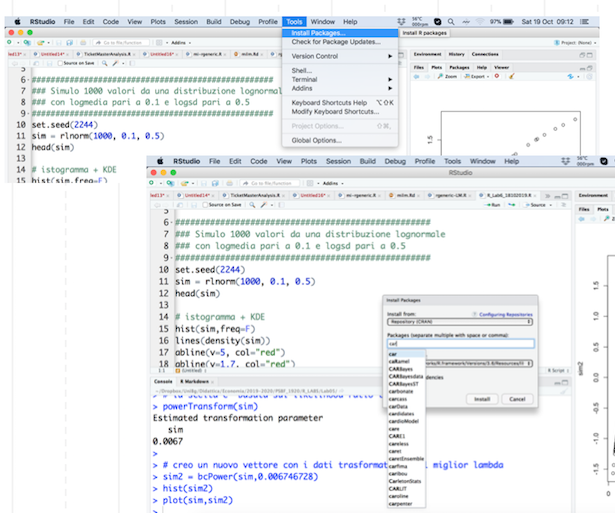
Figure 6.2: The Install Package feature of RStudio
Once the fGarch package is loaded, we are ready to use the function dstd contained in the package.
We proceed similarly to the case of the Normal PDF by using the same sequence of \(x\) values and the parameter estimates contained in fitT:
library(fGarch)
densT = dstd(xseq,
          mean=fitT$estimate[1],
          sd=fitT$estimate[2],
          nu=fitT$estimate[3])
This is the final plot with the KDE and the two fitted PDFs:
plot(density(logret),
     col="blue", ylim=c(0,60))
lines(xseq,densN,col="red")
lines(xseq,densT,col="orange")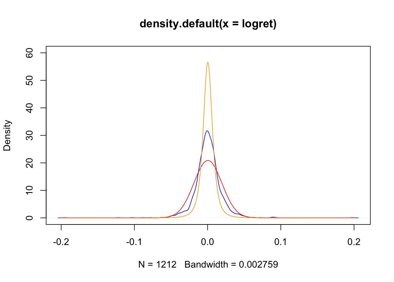
The t distribution is more peaked than the normal model and it fits the data best, as shown by the AIC and BIC indexes. Still it is not a perfect model and it does not perfectly fit the data.
6.3 Exercises lab 4
6.3.1 Exercise 1
Import in R the data available in the GDAXI.csv file. The data refer to the DAX index which is computed considering 30 major German companies trading on the Frankfurt Stock Exchange.
Plot the time series of
Adj.Closeprices (with dates on the x-axis). Do you think the price time series is stationary in time?Compute the DAX gross returns and plot the obtained time series. Do you think the return time series is stationary in time?
Use the histogram to study the gross returns. Add to the histogram the KDE lines for three different bandwidth values (the default one, 1/10 of the default one and 10 times the default one). Comment the effect of changing the bandwidth parameter.
Plot the empirical cumulative density function (ECDF) of the gross returns distribution.
- Evaluate the ECDF for \(x=0.98\) and \(x=1.02\). What’s the meaning of the output you get? Add these values in the ECDF plot.
6.3.2 Exercise 2
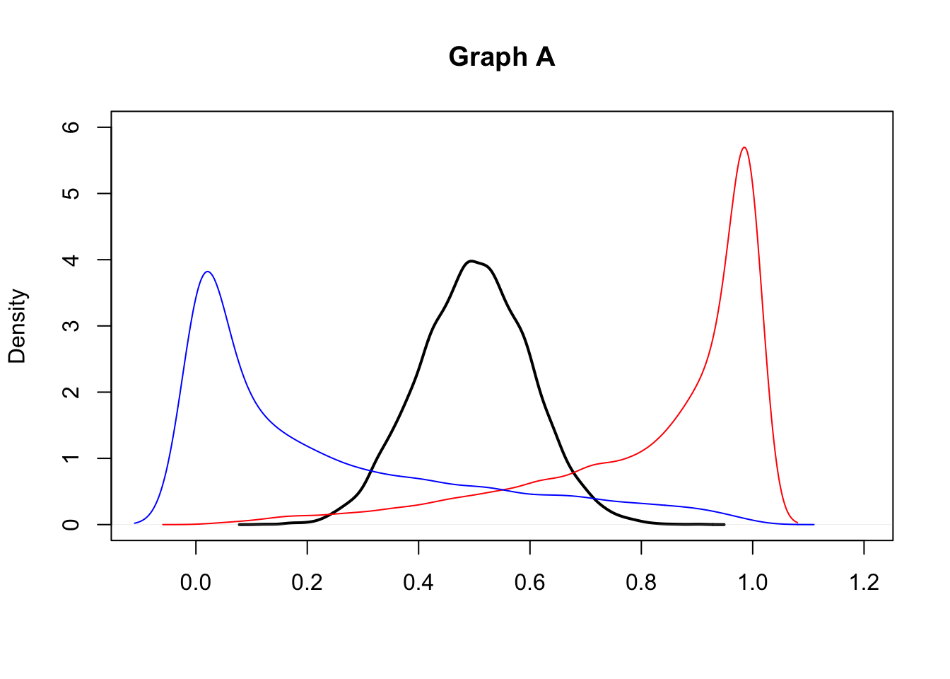
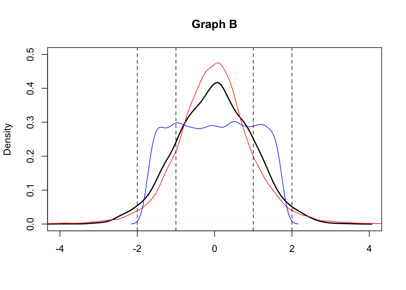
- Consider the following graphs (A and B). They both display the kernel density estimates for three empirical distributions (black, red and blue curves). With regard to graph A what can you comment on the symmetry of the distributions? And for graph B what can you say about kurtosis?
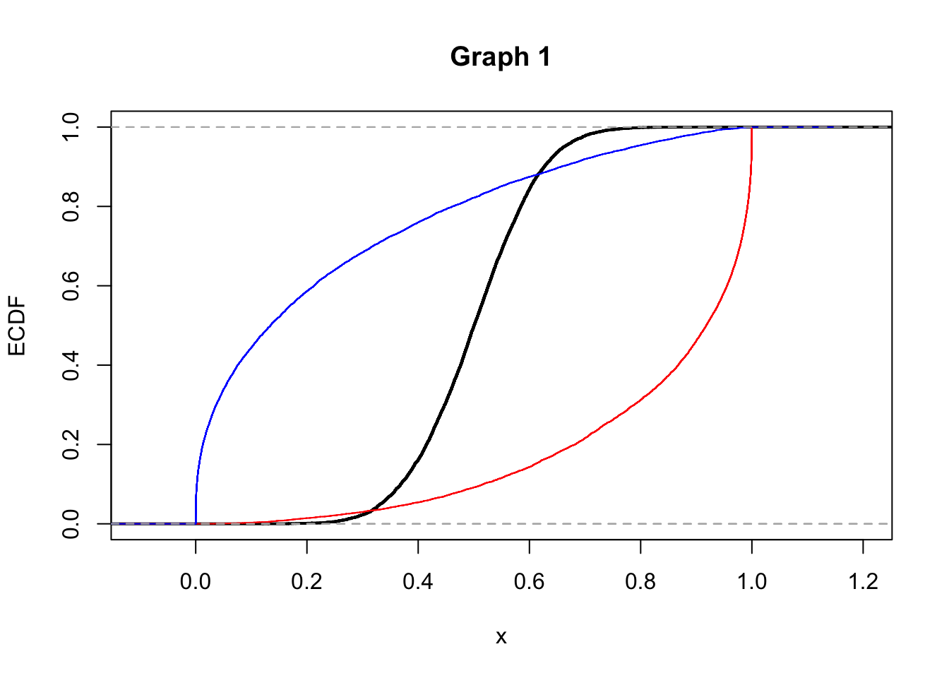
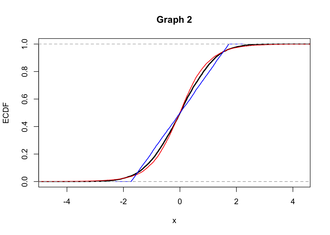
2.Consider the following graphs now (Graph 1 and 2) that display the empirical cumulative density funcitons (ECDF). Does Graph 1 refer to the distributions shown in graph A or in graph B? Explain.
6.3.3 Exercise 3
The daily time series of prices for the ENI asset are available in the file named E.csv (from 2012-11-09 to 2017-11-09). Import the data.
Compute the gross returns (by using Adj.Close prices). Represent the gross returns distribution with an histogram. Comment the plot.
Provide the KDE plot. Moreover, add to the plot the Normal and t PDFs whose parameters have been estimated at the previous point.
Which is the value of the fitted Normal and t PDFs for \(x=0.9\)? Are they similar?
Lists are another kind of objects for data storage. Lists have elements, each of which can contain any type of R object, i.e. the elements of a list do not have to be of the same type.↩︎