Chapter 8 Lab 6 - 16/11/2021
In this lecture we will
- learn how to perform normality test, i.e. Jarque-Bera Test and Shapiro-Wilk test
- we will study the general class of goodness-of-fit test and investigate the difference between simple and composite null hypothesis
- descriptive analysis of a multiple data.frame. How to compute the mean and the variance of a linear combination of random variables (e.g., a portfolio)
8.1 Analysis of the Current Population Survey data
We will use the data stored in the CPSch3.csv file and collected through the Earnings from the Current Population Survey (CPS). The available variables are the following:
year: survey year (quantitative discrete variable)ahe: average hourly earnings (quantitative continuous variable)sex: a qualitative variable with two categories/levels (male,female)
We start with data import and structure check:
CPSch3 = read.csv("files/CPSch3.csv", sep=";")
str(CPSch3)
## 'data.frame': 11130 obs. of 3 variables:
## $ year: int 1992 1992 1992 1992 1992 1992 1992 1992 1992 1992 ...
## $ ahe : num 13 11.6 17.4 10.1 16.7 ...
## $ sex : chr "male" "male" "male" "female" ...For year and sex it is possible to obtain the univariate frequency distribution which reports how many observations are available for each year/category:
table(CPSch3$year)##
## 1992 1994 1996 1998
## 2962 2956 2609 2603table(CPSch3$sex)##
## female male
## 5174 5956We observe, for example, that for year 1992 there are 2962 observations (26.61% of the total number of observations). Moreover, also the bivariate frequency distribution can be easily obtained using the same function:
table(CPSch3$year, CPSch3$sex)##
## female male
## 1992 1371 1591
## 1994 1358 1598
## 1996 1235 1374
## 1998 1210 1393The previous table, is also called contingency table and it reports the joint absolute frequencies of the statistical variables (sex,year). We can also compute the table of the joint relative frequencies of the variable
n_obs <- length(CPSch3$year)
joint_rel<-table(CPSch3$year, CPSch3$sex)/n_obs

joint_rel
##
## female male
## 1992 0.1231806 0.1429470
## 1994 0.1220126 0.1435759
## 1996 0.1109614 0.1234501
## 1998 0.1087152 0.1251572It is worth mentioning that the relative joint frequencies are an estimation of the joint distribution of the random variables (\(Y_1\)=sex, \(Y_2\)=year). Observe for instance that
sum(joint_rel)## [1] 1At the margin of the table we can report the marginal distribution of the two variables
addmargins(joint_rel)##
## female male Sum
## 1992 0.1231806 0.1429470 0.2661276
## 1994 0.1220126 0.1435759 0.2655885
## 1996 0.1109614 0.1234501 0.2344115
## 1998 0.1087152 0.1251572 0.2338724
## Sum 0.4648697 0.5351303 1.0000000Going back at the contingency table, we note that 1371 observations refer to female in year 1992, corresponding to the 46.29% of the observations available for 1992 and to 26.5% of the female data.
In the following we will consider a subset of the original data, referring only to males and observations after 1994. This selection can be performed by setting (logical) conditions are shown in Section 3.2, or by using the subset function as follows:
CPS = subset(CPSch3, sex=="male" & year>1994)
dim(CPS)
## [1] 2767 3head(CPS)## year ahe sex
## 5920 1996 11.660622 male
## 5922 1996 14.971988 male
## 5923 1996 25.958241 male
## 5924 1996 9.989918 male
## 5925 1996 13.451954 male
## 5926 1996 21.394132 malestr(CPS)## 'data.frame': 2767 obs. of 3 variables:
## $ year: int 1996 1996 1996 1996 1996 1996 1996 1996 1996 1996 ...
## $ ahe : num 11.66 14.97 25.96 9.99 13.45 ...
## $ sex : chr "male" "male" "male" "male" ...The new data frame, named CPS, contains 2767 observations.
We analyze and represent graphically the only continuous variable available in the data frame:
summary(CPS$ahe)## Min. 1st Qu. Median Mean 3rd Qu. Max.
## 2.159 12.009 16.233 17.416 21.377 52.467hist(CPS$ahe)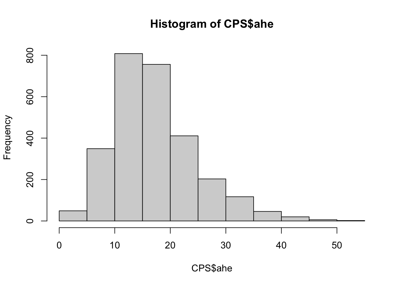
The distribution appears to hava a positive skewness; this is confirmed by the fact that the mean is greater than the median and by the following normal probability plot with a concave pattern:
qqnorm(CPS$ahe,datax=T)
qqline(CPS$ahe,datax=T)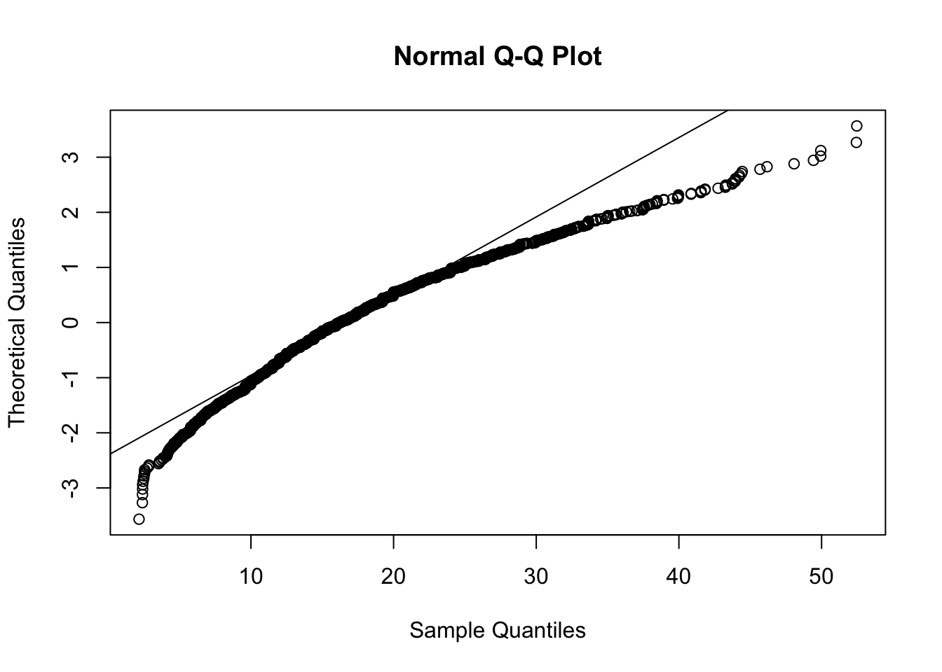
8.2 Normality tests
The aim of normality tests is to assess the normality of a set of observed data. Thus, the null hypothesis is \(H_0\):data are from a Normal distribution, against the alternative hypothesis \(H_1\):data are not from a Normal distribution. A decision is taken by using the p-value.
In the following we present the Jarque-Bera and Shapiro-Wilk tests.
8.2.1 Jarque-Bera Normality test
The Jarque-bera test of normality uses the sample skewness \(\hat{Sk}\) and kurtosis \(\hat{Kur}\) which are compared with the corresponding expected value (0 and 3) in case of Normal distribution. The test statistic is given by \[ JB = n\left(\frac{\hat{Sk}^2}{6}+\frac{(\hat{Kur}-3)^2}{24}\right) \] which, under the null hypothesis, is approximately distributed like a Chi-square distribution with 2 degrees of freedom (\(\chi^2_2\)). Under the null hypothesis (normality), we expect a value of the test statistic close to 0.
This test is implemented in R using the jarque.bera.test function which is part of the tseries package.
Assuming that the tseries package is already installed (see Section 6.2.3.1), we load it and run the test for the ahe variable:
library(tseries)## Registered S3 method overwritten by 'quantmod':
## method from
## as.zoo.data.frame zoojarque.bera.test(CPS$ahe)##
## Jarque Bera Test
##
## data: CPS$ahe
## X-squared = 570.37, df = 2, p-value < 2.2e-16Given the extremely small value of the p-value (basically equal to zero), we reject, as expected given the plots, the normality hypothesis which is not supported by the data.
It is also possible to compute the value of the test statistic manually. Nevertheless, since to compare our results with the one obtained with the jarque.bera.test, we need to compute the Skewness and the Kurtosis statistics using the population standard deviation (we have programmed an R function in Section 7.2. Then we first define the function to compute the population standard deviation
sd_pop<- function(y){
        n<- length(y)
        output<- sqrt( (n-1)/n )*sd(y)
        return(output)
}
Then we will compute the JB test statistics as follows
n = length(CPS$ahe)
sk = mean((CPS$ahe-mean(CPS$ahe))^3)/sd_pop(CPS$ahe)^3
kur = mean((CPS$ahe-mean(CPS$ahe))^4)/sd_pop(CPS$ahe)^4
JB = n*(sk^2/6+(kur-3)^2/24)
JB
## [1] 570.3726The corresponding p-value can be computed manually by using the pchisq function which provides the cumulative distribution function (i.e. \(P(X\leq x)\)) for a random variable \(X\) which is distributed like a Chi-square Distribution with df degrees of freedom. In this case df=2. We should also remember that the critical region of a JB test is unilateral on the right:
pchisq(JB,df=2,lower.tail = F)## [1] 1.39688e-124The option lower.tail = F because we are interested in the probability in the right tail, while pchisq returns the probability in the left side. As an alternative we could have computed the complement at one of the pchisq, i.e.,
1-pchisq(JB,df=2)## [1] 0As described in Section 7.4, we use the Box-Cox transformation to solve the asymmetry issue. The transformed variable, named ahe2, is added to the data frame:
library(car)
bestpar = powerTransform(CPS$ahe)
bestpar$lambda
## CPS$ahe
## 0.3531166CPS$ahe2 = bcPower(CPS$ahe,bestpar$lambda)
head(CPS)## year ahe sex ahe2
## 5920 1996 11.660622 male 3.909613
## 5922 1996 14.971988 male 4.531714
## 5923 1996 25.958241 male 6.111130
## 5924 1996 9.989918 male 3.551352
## 5925 1996 13.451954 male 4.258539
## 5926 1996 21.394132 male 5.520853The transformed variable distribution is studied here below by means of different plots:
hist(CPS$ahe2,freq=F)
lines(density(CPS$ahe2),col="red")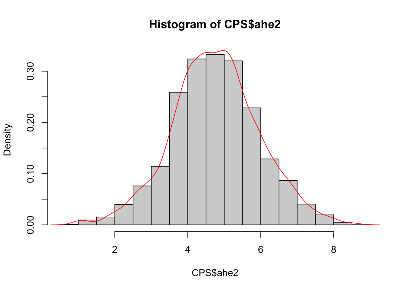
qqnorm(CPS$ahe2,datax = T)
qqline(CPS$ahe2,datax = T,col="red")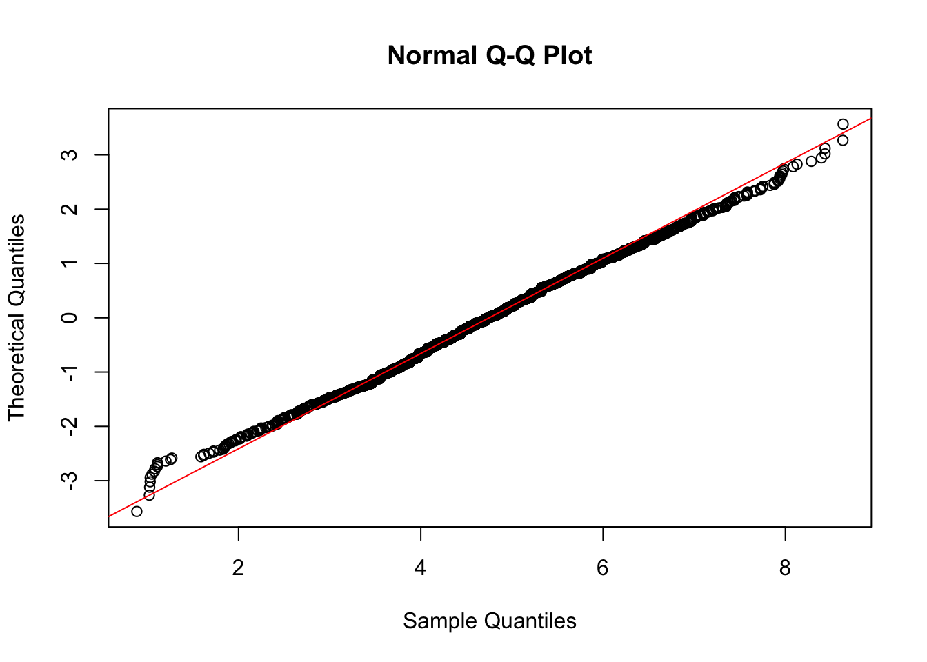
Figure 8.1: Normal probability plot of the transformed data
The distribution seems to be symmetric and most of the points in the normal probability plot have a linear pattern, but with some points that deviate from the reference line in the left and right tails. Can we conclude that the transformed data are normally distributed? We will use a (different) normality test.
8.2.2 Shapiro-Wilk Normality test
The Shapiro-Wilk is based on the correlation between the empirical quantiles, given by the sample order statistics \(y_{(i)}\), and the theoretical Normal quantiles \(z_{(i)}=E(Z_{(i)})\). Under normality, the correlation should be close to 1; the \(H_0\) hypothesis of normality is rejected for small values of the test statistic.
The shapiro.test function is part of the base R release and provides the values of the test statistic and of the corresponding p-value. It can be computed only if the sample size (\(n\)) is lower than 5000.
shapiro.test(CPS$ahe2)##
## Shapiro-Wilk normality test
##
## data: CPS$ahe2
## W = 0.99775, p-value = 0.0005052In this case, even if the correlation coefficient (0.9977467) is close to 1, the p-value is quite small and leads to the rejection of the normality hypothesis. Note that the Shapiro-Wilk test is known to be a sample-size biased test: for big sample even small differences from the Normal distribution lead to the rejection of the \(H_0\) hypothesis. In this case deviations from the Normal distribution are observed in the tails (see Figure 8.1).
Let’s try to use the Jarque-Bera test for the same set of data:
jarque.bera.test(CPS$ahe2)##
## Jarque Bera Test
##
## data: CPS$ahe2
## X-squared = 6.2297, df = 2, p-value = 0.04439In this case the p-value does not provide a very strong evidence against \(H_0\) (if compared with the p-value of the Shapiro-Wilk test). However, if we set the significance level \(\alpha\) (type I error probability) to 0.05, we reject the normality hypothesis also in this case.
8.3 Goodnes of fit test
8.4 Kolmogorov-Smirnov test
This test compares the empirical CDF \(F_n(t)\) (ECDF, see Section 6.1) and the theoretical CDF \(F(t)\) of a continuous random variable whose (population) parameters are assumed to be known. The test statistics is given by the absolute distance between the two function defined as follows: \[ D_n=\sup_t |F_n(t)-F(t)| \]
Under the null hypothesis, we expect a small value of \(D_n\). In R the ks.test(x,y,...) function can be used to perform this test. The following arguments have to be specified:
xis the vector of datayis a string naming a theoretical CDF, as for instancepnormfor the Normal distribution,plnormfor the logNormal distribution....is used to specify the parameters of the considered distribution (for examplemean=...andsd=...ifpnormis used, ormeanlog=...andsdlog=...ifplnormis used).
However there is an issue with the Kolmogorov-Smirnov test implemented in ks.test. As reported in its help page “the parameters specified in … must be pre-specified and not estimated from the data”.
In other words, it is not possible to specify a “composite” null hypothesis with the ks.test function.
The point is that when the hypothesis is composite, we need to use the sample data to estimate the population parameters. When we plug-in the test the estimated parameters, the Kolmogorov-Smirnov test statistic is closer to the null distribution than it would be when the population parameters are known (and this results in increased Type II error probability, i.e. of the probability of not rejecting \(H_0\) when it is not true). See, for example, the following case where we simulate 200 values from the Uniform(0,1) distribution (see here for the definition of continuos Uniform distribution) by using the runif function:
set.seed(4)
x = runif(200)
hist(x)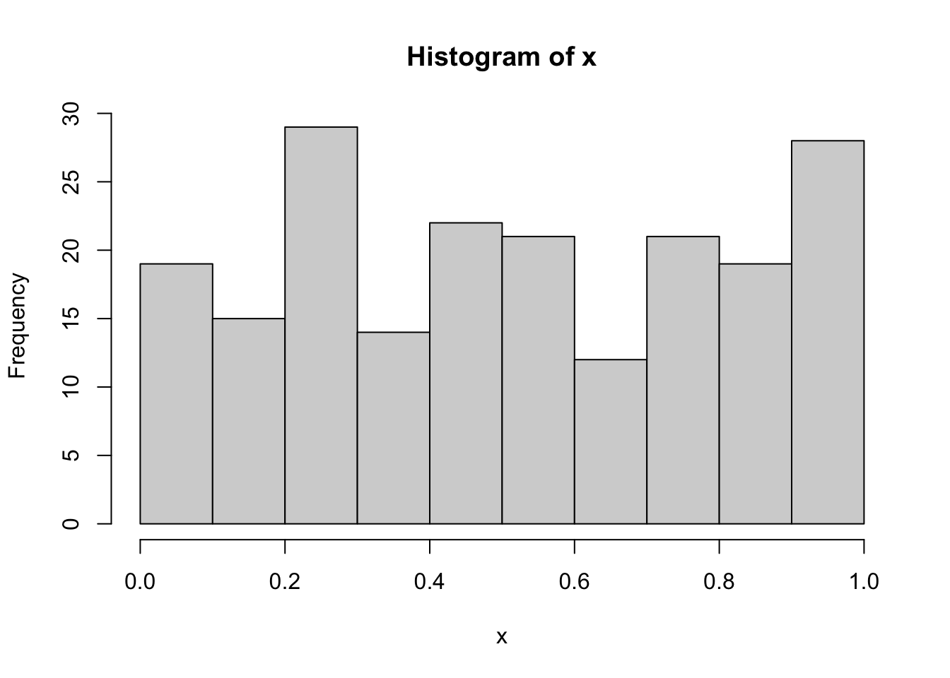
The data aren’t for sure normally distributed because they were simulated from the Uniform distribution. However, if we run the Kolmogorov-Smirnov test with ks.test and by using the sample statistics (mean and sd), we obtain
ks.test(x, "pnorm",
        mean=mean(x),
        sd=sd(x))
##
## One-sample Kolmogorov-Smirnov test
##
## data: x
## D = 0.089686, p-value = 0.08011
## alternative hypothesis: two-sidedThe p-value is 0.0801094: if we consider as threshold 0.05, we conclude the data suggest to not reject the normality hypothesis (and we know this is a wrong decision, i.e. second type error).
To overcome this issue it is possible to use the corrected version of the Kolmogorov-Smirnov test by means of the LcKS function included in the KScorrect library (that has to be installed and then loaded):
library(KScorrect)
ks2 = LcKS(x,"pnorm", parallel = TRUE)
## Warning in LcKS(x, "pnorm", parallel = TRUE): Consider setting 'parallel =
## FALSE' to increase the speed of this function.## LcKS is running in parallel with 3 worker(s) using doParallelSNOW [1.0.16]ks2$p.value## [1] 6e-04In this case the p-value leads to correctly reject the normality assumption for the data contained in x.
Let’s now consider one of the quantitative variable in datareg and check if we can be considered as generated from the Normal model:
#nasdaq_KS = LcKS(datareg$ibm,"pnorm")
#nasdaq_KS$p.value
Given the small p-value we reject the normality hypothesis; this conclusion is coherent with the features of the distribution represented in the following plots:
#plot(density(datareg$ibm))
#qqnorm(datareg$ibm, datax=T)
#qqline(datareg$ibm, datax=T)
8.4.1 Other gof-test
The Cramér–von Mises test (CVM-test) is an other goodness-of-fit test whose statistics is a distance between the empirical distribution of the data \({\displaystyle F_{n}}\) and a theoretical distribution \(F\), i,e,The test statistics is \[ {\displaystyle \omega ^{2}=\int _{-\infty }^{\infty }[F_{n}(x)-F(x)]^{2}\,\mathrm {d} F(x)} \]
The Anderson–Darling test (AD-test), again is goodness-of-fit test whose statistics is a distance between the empirical distribution of the data \({\displaystyle F_{n}}\) and a theoretical distribution \(F\). When applied to testing whether a normal distribution adequately describes a set of data, it is one of the most powerful statistical tools for detecting most departures from normality.
The Anderson–Darling test statistics \[ {\displaystyle A^{2}=n\int _{-\infty }^{\infty }{\frac {(F_{n}(x)-F(x))^{2}}{F(x)\;(1-F(x))}}\,dF(x),} \]
In R the test both the CVM-test and the AD-test are implemented in the library goftest. The two main function are cvm.test and ad.test.
By default, each test assumes that the parameters of the null distribution are known (a simple null hypothesis). If the parameters were estimated (calculated from the data) then the user should set estimated=TRUE which uses a method adjust for the effect of estimating the parameters from the data (i.e. it adjust the p-value for composite null hypothesis)
8.4.2 Gof test for three set of data
As an example we are going to analyze the other set of data, that we already have seen in class: the magenta (file magenta_data.txt), the green (file green_data.txt), and the cyan data (file cyan_data.txt)
Let’s load the data and produce some of the plot that we know already. Observe that, since the files contain an univariate sequence of data, we can use the function scan to inport the data.
Magenta data
series1 <- scan(file="files/magenta_data.txt")

par(mfrow=c(1,3))
hist(series1,freq=F,col="magenta")
boxplot(series1,col="magenta")
qqnorm(series1,datax = T,col="magenta",pch="*",cex=1.5)
qqline(series1,datax=T)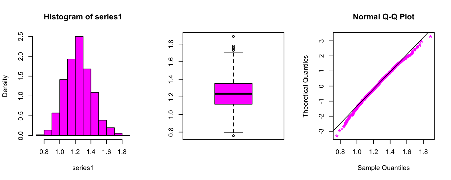
Summary statistics of the Magenta data
summary(series1)## Min. 1st Qu. Median Mean 3rd Qu. Max.
## 0.7596 1.1169 1.2362 1.2409 1.3530 1.8869For this set of data we want to perform the following test: \[ H_0:\text{Data have been generated from a Gamma distribution} \]
To perform the test we need to estimate the parameter \(\alpha\), i.e. the shape, and the parameter \(\beta\), i.e., the rate, of the Gamma distribution, given the observation.
We will perform the estimation via the
fitdistr of the MASS library
library(MASS)
fitN = fitdistr(x=series1,densfun="gamma")
fitN
## shape rate
## 52.199691 42.066751
## ( 2.326943) ( 1.884256)Then we can compute the p-value for the three gof-test we have studied
Kolmogorov-Smirnov
ks2 = LcKS(series1,"pgamma")## Warning in LcKS(series1, "pgamma"): Consider setting 'parallel = TRUE' to
## increase the speed of this function.#ks2$p.value
0.6448## [1] 0.6448Anderson-Darling
library(goftest)
ad.test(series1, "pgamma", shape=fitN$estimate["shape"],
        rate=fitN$estimate["rate"], estimated=TRUE)
##
## Anderson-Darling test of goodness-of-fit
## Braun's adjustment using 32 groups
## Null hypothesis: Gamma distribution
## with parameters shape = 52.1996908290833, rate = 42.0667510631009
## Parameters assumed to have been estimated from data
##
## data: series1
## Anmax = 5.1624, p-value = 0.07556Cramer-von Mises
cvm.test(series1, "pgamma", shape=fitN$estimate["shape"],
        rate=fitN$estimate["rate"], estimated=TRUE)
##
## Cramer-von Mises test of goodness-of-fit
## Braun's adjustment using 32 groups
## Null hypothesis: Gamma distribution
## with parameters shape = 52.1996908290833, rate = 42.0667510631009
## Parameters assumed to have been estimated from data
##
## data: series1
## omega2max = 0.91382, p-value = 0.1089In the three cases we obtained large p-value, suggesting an data evidence in favour of the null hypotesis, indeed we conclude that a Gamma model fits well the data.
Green data
series2 <- scan("files/green_data.txt")


par(mfrow=c(1,3))
hist(series2,freq=T,col="green")
boxplot(series2,col="green")
qqnorm(series2,datax = T,col="green",pch="*",cex=1.5)
qqline(series2,datax=T)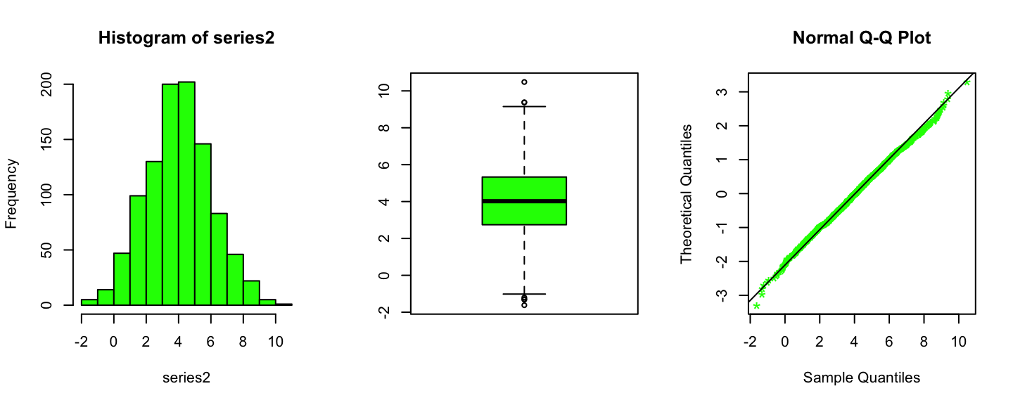
Summary statistics of the Green data
summary(series2)## Min. 1st Qu. Median Mean 3rd Qu. Max.
## -1.620 2.743 4.018 4.032 5.329 10.482For this set of data we want to perform the following test: \[ H_0:\text{Data have been generated from a Normal distribution} \]
To perform the test we need to estimate the parameter \(\mu\), i.e. the mean, and the parameter \(\sigma\), i.e., the standard deviation, of the Normal distribution, given the observation. In this case they corresponds with the sample mean and with the sample standard deviation
library(MASS)
hat_mu<- mean(series2)
hat_sig <- sd(series2)
Then we can compute the p-value for the three gof-test we have studied
Kolmogorov-Smirnov
ks2 = LcKS(series1,"pnorm",parallel = T)## Warning in LcKS(series1, "pnorm", parallel = T): Consider setting 'parallel =
## FALSE' to increase the speed of this function.## LcKS is running in parallel with 3 worker(s) using doParallelSNOW [1.0.16]ks2$p.value## [1] 0.0282Anderson-Darling
ad.test(series2, "pnorm", mean=hat_mu,
        sd=hat_sig, estimated=TRUE)
##
## Anderson-Darling test of goodness-of-fit
## Braun's adjustment using 32 groups
## Null hypothesis: Normal distribution
## with parameters mean = 4.03225574117, sd = 1.98338995259963
## Parameters assumed to have been estimated from data
##
## data: series2
## Anmax = 3.5744, p-value = 0.3694Cramer-von Mises
cvm.test(series2, "pnorm", mean=hat_mu,
        sd=hat_sig, estimated=TRUE)
##
## Cramer-von Mises test of goodness-of-fit
## Braun's adjustment using 32 groups
## Null hypothesis: Normal distribution
## with parameters mean = 4.03225574117, sd = 1.98338995259963
## Parameters assumed to have been estimated from data
##
## data: series2
## omega2max = 0.50485, p-value = 0.7108Cyan data
series3 <- scan(file="files/cyan_data.txt")

par(mfrow=c(1,3))
hist(series3,freq=T,col="cyan")
boxplot(series3,col="cyan")
qqnorm(series3,datax = T,col="cyan",pch="*",cex=1.5)
qqline(series3,datax=T)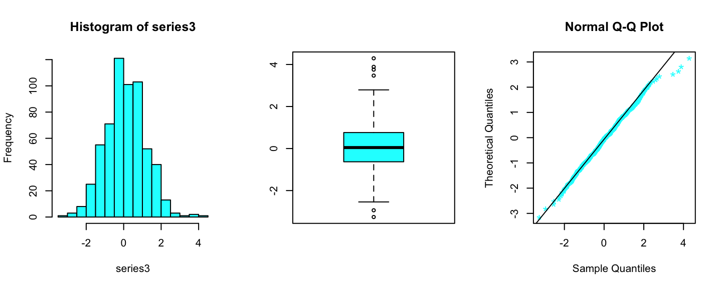
Summary statistics cyan data
summary(series3)## Min. 1st Qu. Median Mean 3rd Qu. Max.
## -3.25854 -0.62827 0.04657 0.10559 0.75867 4.29380For this set of data we want to perform the following test: \[ H_0:\text{Data have been generated from a t-student distribution} \]
To perform the test we need to estimate the parameter \(\mu\), i.e. the non-central (or location) parameter the parameter \(\sigma\), i.e., scale parameter, and the parameter \(\nu\), i.e. the degrees of freedom of the t-student distribution, given the observation.
To this end we will use the
fitdistr function of the MASS library
library(MASS)
fitN = fitdistr(x=series1,densfun="t")
fitN
## m s df
## 1.240266e+00 1.692066e-01 6.969612e+01
## (5.501338e-03) (5.403389e-03) (1.107708e+02)Nevertheless, we should observe that the R built-in function pt, is parametrized only respect to \(\mu\) and \(\nu\).
To apply the gof-test implemented in the goftest we have to take into account the lack of \(\sigma\). To this end we can observe that if \(X\sim\)t-student\((\mu,\sigma,\nu)\) then
if we let \(Y=X/\sigma\) we have that \(Y\sim\)t-student\((\mu/\sigma,1,\nu)\), so we can apply the test on the transformed data.
So we tranform the data
series3_tran <- series3/fitN$estimate["s"]And we apply the Anderson-Darling test to the tranformed data
ad.test(series3_tran, "pt", df=20.17,
        ncp=fitN$estimate["m"]/fitN$estimate["s"],
        estimated=TRUE)
##
## Anderson-Darling test of goodness-of-fit
## Braun's adjustment using 24 groups
## Null hypothesis: Student's t distribution
## with parameters df = 20.17, ncp = 7.32988991315944
## Parameters assumed to have been estimated from data
##
## data: series3_tran
## Anmax = 418.58, p-value = 0.0005758In the same way we apply the Cramer-von Mises test to the tranformed data
cvm.test(series3_tran, "pt", df=20.17,
         ncp=fitN$estimate["m"]/fitN$estimate["s"],
         estimated=TRUE)
##
## Cramer-von Mises test of goodness-of-fit
## Braun's adjustment using 24 groups
## Null hypothesis: Student's t distribution
## with parameters df = 20.17, ncp = 7.32988991315944
## Parameters assumed to have been estimated from data
##
## data: series3_tran
## omega2max = 7.3789, p-value < 2.2e-16We obtained quite large values of the p-value, and we can conclude that there is not evidence to reject the null hypothesis, so we conclude that the cyan data are distributed according to a t-student distribution.
8.5 Joint analysis of the assess of four different stocks
The file
prices.txt contain daily prices of the following stocks (from 2020-11-05, to 2021-11-03):
- ge General Electrics
- nok Nokia
- nok Facebook
- sp Standard and Poor (SP)
Let’s clear the R-worksheet and load the data
###
rm(list=ls())
prices<- read.table("files/prices.txt",header=T)
str(prices)
## 'data.frame': 247 obs. of 5 variables:
## $ Date: chr "2020-11-05" "2020-11-06" "2020-11-09" "2020-11-10" ...
## $ ge : num 63.7 64.5 69.5 71.6 70.9 ...
## $ nok : num 3.54 3.52 3.65 3.67 3.75 3.75 3.81 3.9 3.93 3.94 ...
## $ face: num 250 248 243 227 234 ...
## $ sp : num 345 345 350 349 352 ...We observe that the firs variable in the data-frame is the day at which the prices have been collected. Nevertheless, R reed this column as of type character chr. A very useful library to transform string (i.e chr object) into dates is lubridate
library("lubridate")
is(prices$Date)
## [1] "character" "vector" "data.frameRowLabels"
## [4] "SuperClassMethod" "index" "atomicVector"prices$Date<-ymd(prices$Date)
is(prices$Date)## [1] "Date" "oldClass" "time_timeSeries"prices$Date[1] #first day of obeservation## [1] "2020-11-05"tail(prices$Date)[1] # last day of observation## [1] "2021-10-27"Let’s give a look at the time series of the prices
par(mfrow=c(2,2))
for(i in 1:4){
plot(prices$Date,prices[,i+1],type="l",
        main=paste("Prices of", names(prices)[i+1]),col=i+1,lwd=2)
}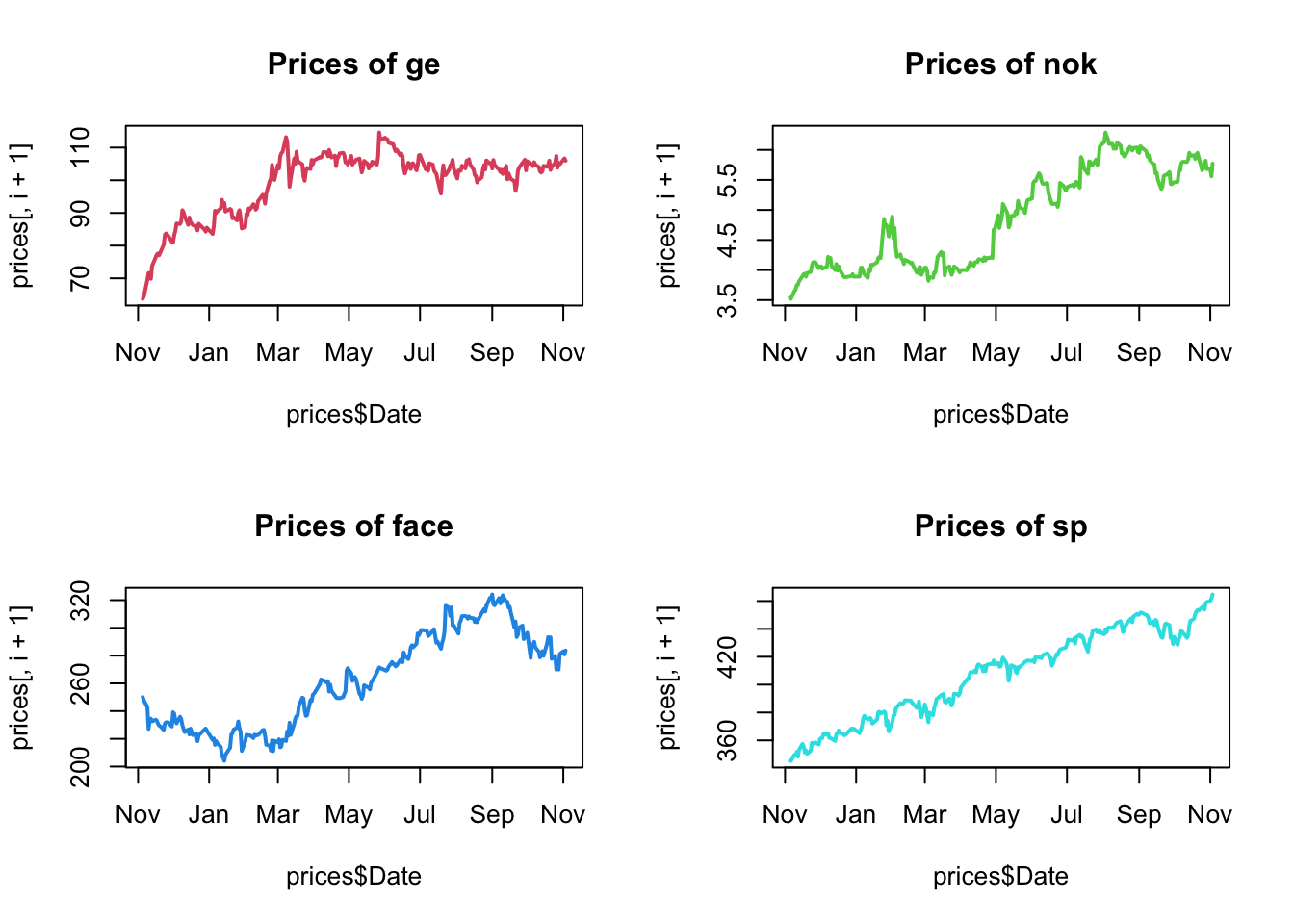
We observe a quite strong “trend” for all the time series, moreover the prices of the different stocks are very different, form the average of 4.8728745$ for a Nokia’s share to the average of 408.0274877$ for a SP’s share
For more information we can look at the univariate or marginal statistics for the four stocks
summary(prices[,-1])## ge nok face sp
## Min. : 63.72 Min. :3.520 Min. :204.1 Min. :345.3
## 1st Qu.: 92.51 1st Qu.:4.060 1st Qu.:229.0 1st Qu.:380.1
## Median :103.44 Median :4.900 Median :261.8 Median :414.1
## Mean : 99.45 Mean :4.873 Mean :262.3 Mean :408.0
## 3rd Qu.:105.70 3rd Qu.:5.670 3rd Qu.:293.1 3rd Qu.:435.4
## Max. :114.62 Max. :6.290 Max. :324.1 Max. :464.7Now we want to study the relationship between the four shares. To this end we compute the Variance-Covariance matrix and the correlation matrix.
Covariance
cov(prices[,-1])## ge nok face sp
## ge 96.596734 4.2184380 172.14966 229.90921
## nok 4.218438 0.6668425 24.80614 23.43198
## face 172.149662 24.8061397 1142.65856 957.33674
## sp 229.909207 23.4319836 957.33674 1007.06617Correlation
cor(prices[,-1])## ge nok face sp
## ge 1.0000000 0.5256042 0.5181634 0.7371335
## nok 0.5256042 1.0000000 0.8986474 0.9042081
## face 0.5181634 0.8986474 1.0000000 0.8924368
## sp 0.7371335 0.9042081 0.8924368 1.0000000Moreover we depict a pairs-plot of the prices of the four stocks
par(mfrow=c(1,1),mar=c(3,3,1,1),mgp=c(1.75,.75,0))
pairs(prices[,-1], main="Pairs of the Prices") 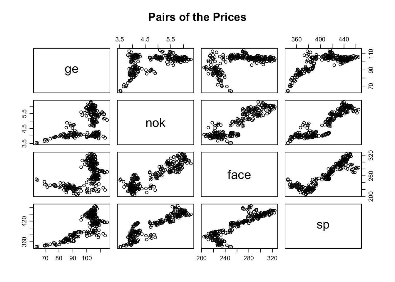
From the pairs plot we can appreciate the dependence between the prices, nevetheless, the dependence is not linear. So the correlation matrix is not properly interpretable, indeed the entries of the matrix measure the linear dependence between the corresponding pair of random variables.
8.5.1 The log Returns
Now we want to compute the log-returns of the four assets. We First compute the log prices
logprices<- log(prices[,-1])Then we apply the function diff to all the
column of logprices to obtain the log-returns
logRet<- apply(logprices,2,diff)We can give a look at the four time-series logreturns
par(mfrow=c(2,2))
for(i in 1:4){
  matplot(prices$Date[-1],logRet[,i],type="l",
          main=paste("log returns of",names(prices)[i+1]),col=i+1,lwd=2)
}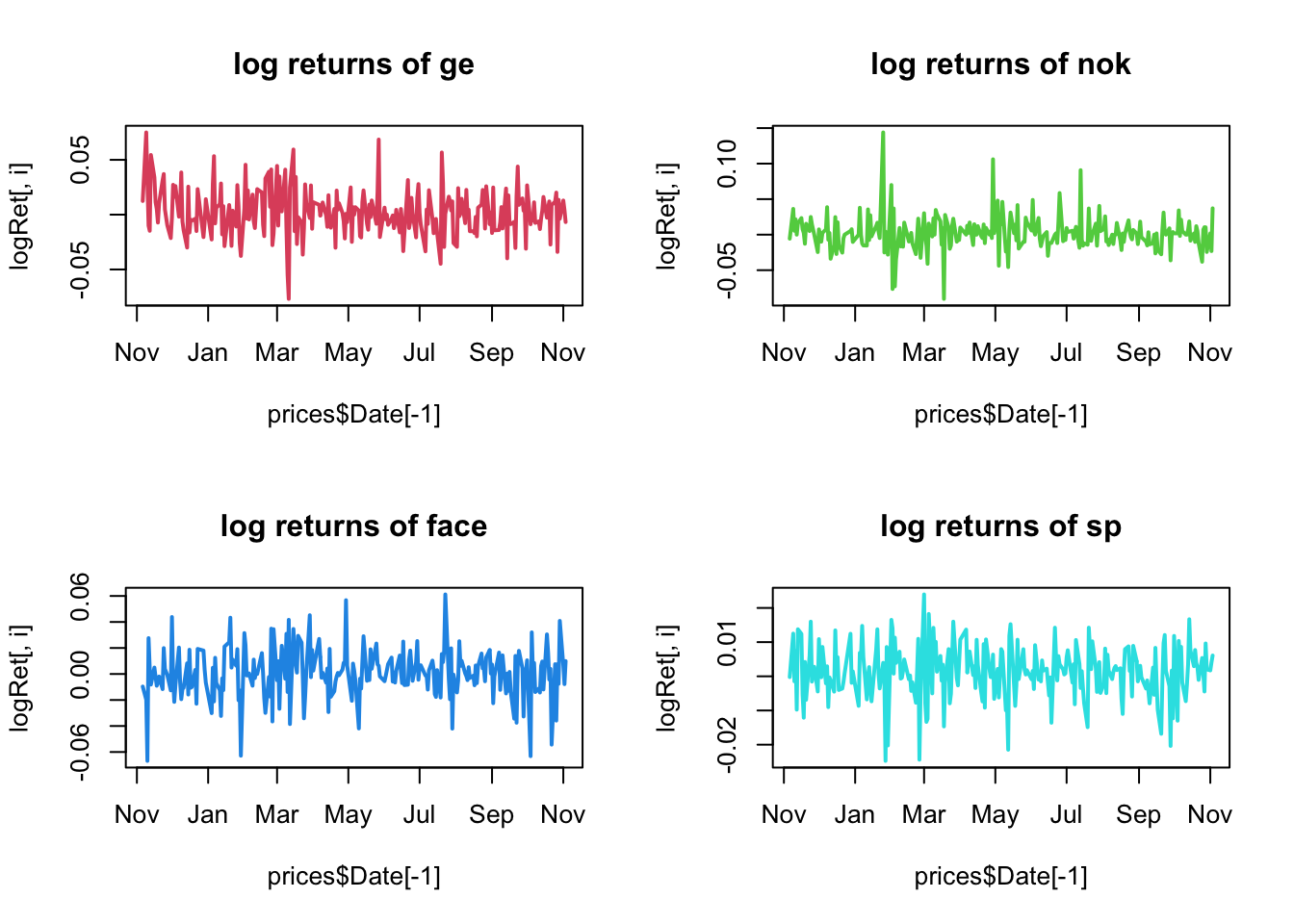
they look much more stationary than the prices.
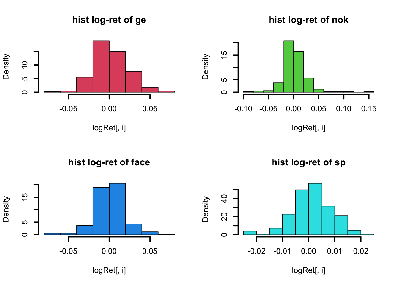
Nevertheless the logReturns ar not really Normal distributed, as we can see from the histogram
par(mfrow=c(2,2))
for(i in 1:4){
  hist(logRet[,i],
          main=paste("hist log-ret of",names(prices)[i+1]),
       col=i+1,lwd=2,freq=F)
}
From the Normal probability plots
par(mfrow=c(2,2))
for(i in 1:4){
  qqnorm(logRet[,i],main=paste("qqnorm log-ret of",names(prices)[i+1]),
       col=i+1,lwd=2,datax = T)
  qqline(logRet[,i],datax=T,lty=2,lwd=2)
}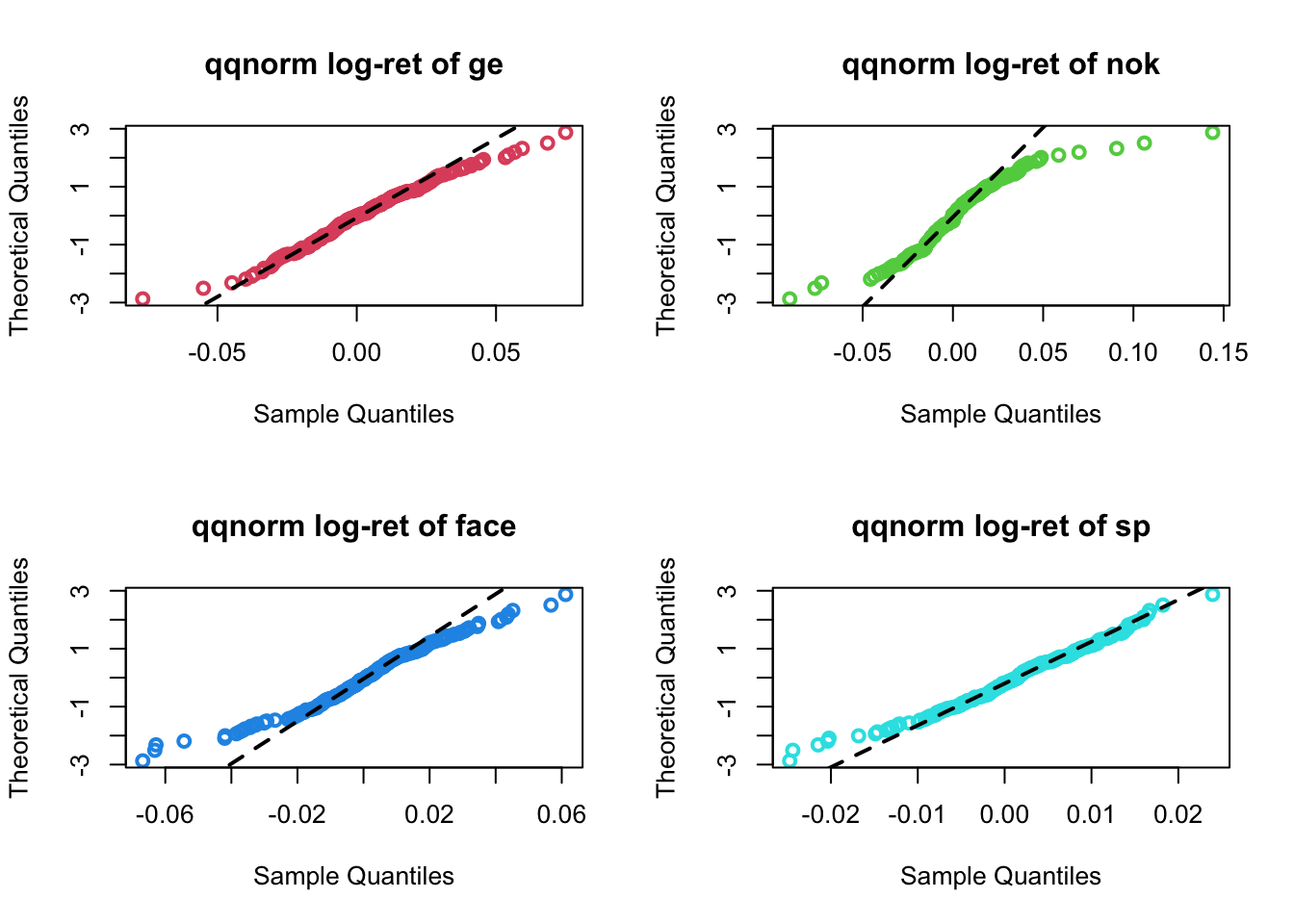
Let’s now give a look at the summary (i.e. at the mariginal statistics), at the covariance and at the correlation matrix of the log-Returns
Summary
summary(logRet)## ge nok face
## Min. :-0.0768403 Min. :-0.090416 Min. :-0.0668334
## 1st Qu.:-0.0110392 1st Qu.:-0.010124 1st Qu.:-0.0086579
## Median : 0.0003787 Median : 0.000000 Median : 0.0007323
## Mean : 0.0020680 Mean : 0.001986 Mean : 0.0005124
## 3rd Qu.: 0.0136856 3rd Qu.: 0.011678 3rd Qu.: 0.0097723
## Max. : 0.0749904 Max. : 0.143894 Max. : 0.0611787
## sp
## Min. :-0.024744
## 1st Qu.:-0.003277
## Median : 0.001519
## Mean : 0.001207
## 3rd Qu.: 0.006059
## Max. : 0.023951Covariance
cov(logRet)## ge nok face sp
## ge 4.499589e-04 7.093867e-05 -2.836971e-05 6.031814e-05
## nok 7.093867e-05 5.694915e-04 6.712406e-05 6.684402e-05
## face -2.836971e-05 6.712406e-05 3.515832e-04 5.875652e-05
## sp 6.031814e-05 6.684402e-05 5.875652e-05 6.015415e-05Correlation
cor(logRet)## ge nok face sp
## ge 1.00000000 0.1401371 -0.07132708 0.3666306
## nok 0.14013706 1.0000000 0.15001010 0.3611488
## face -0.07132708 0.1500101 1.00000000 0.4040259
## sp 0.36663056 0.3611488 0.40402587 1.0000000To better understand the correlation matrix we can produce a pairs plot, that is a scatter-plot between all the pairs of variables in the data.frame
Paris of the log-returns
par(mfrow=c(1,1),mar=c(3,3,1,1),mgp=c(1.75,.75,0))
pairs(logRet, main="Pairs of the log-returns")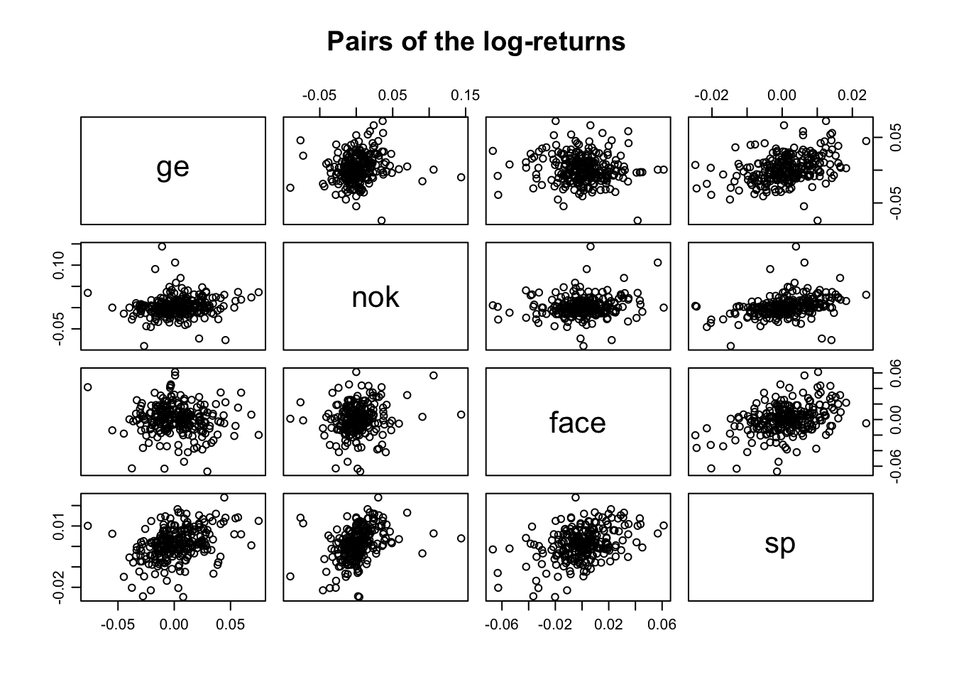
The sequences of log-returns are weekly correlated. Indeed, we can appreciate a week linear trend between the log-returns in the by looking at the pairs plot.
8.6 Portfolio
Suppose that at the 5\(^{th}\) of November 2020 we had around 2000$ that we want to invest. In particular we want to invest on Facebook, General Electric and Nokia.
Let’s start by looking at the prices of the three stocks at the “2020-11-05”
price_port<- prices[1,c("face","ge","nok")]
price_port
## face ge nok
## 1 250.1 63.71612 3.54Suppose now we want to differentiate our investment by putting 1000 $ on Facebook, 700$ on General Electric, and 300$ on Nokia.
So the budget is split as follow
budget<- c(1000,700,300)Now we have to compute how many share of each stock we can buy with our budget
shares<- round(budget/price_port,0)
shares
## face ge nok
## 1 4 11 85Indeed the total money I have to invest is
total_inve =sum(shares*price_port)
total_inve
## [1] 2002.177We have got a portfolio. I want to compute how much each stock weight in it. That is the weigth of the value of each stock compared with the total money that I have invested:
w=as.numeric((shares*price_port)/total_inve)
w
## [1] 0.4996561 0.3500576 0.1502864After observing the prices of the three stocks for one year, I cam compute the mean of the daily log return of the portfolio.
mean_por<- t(w)%*%colMeans(logRet[,c("face","ge","nok")])
mean_por
## [,1]
## [1,] 0.001278404Variance of log-returns in the portfolio
var_por<-t(w)%*%cov(logRet[,c("face","ge","nok")])%*%w
var_por
## [,1]
## [1,] 0.0001633963Coefficient of variation
cv_por<- sqrt(var_por)/mean_por8.7 Exercises Lab 6
8.7.1 Exercise 1
The daily time series of prices for the ENI asset are available in the file named E.csv (from 2012-11-09 to 2017-11-09). Import the data.
Compute the gross returns (by using Adj.Close prices). Represent the gross returns distribution with an histogram. Comment the plot.
Test the normality of the gross returns distribution.
Fit the Normal and t distribution to the data. Provide the estimated parameters. Moreover, which is the best model by using the deviance, the AIC and BIC?
Provide the KDE plot. Moreover, add to the plot the Normal and t PDFs whose parameters have been estimated at the previous point.
Which is the value of the fitted Normal and t PDFs for \(x=0.9\)? Are they similar?
8.7.2 Exercise 2
Simulate 1000 values from the logNormal distribution with with parameters equal to 15 (meanlog) and 0.5 (varlog). Use the value 789 as seed.
Plot the data using the boxplot and the normal probability plot.
Fit to the data a distribution. You have to choose which theoretical distribution, but knowing where the data come from it’s easy. See also the available distributions in
?fitdistr. Which are the estimated parameters?Plot the KDE of the simulated data together with the fitted PDF. To compute the latter, for a reasonable sequence of \(x\) values, you will have to use a function in R whose names starts with
d....Fit to the data the Exponential distribution (see here. You will have to use
densfun=exponentialinfitdistr. Provide the parameter estimates.In terms of deviance, AIC and BIC which is the best model?
8.7.3 Exercise 3
The file prices_ex.cs contains the daily prices of three different stocks of the USA market: Google (GOG), Amazon (AMZN) and Tesla (TSLA). In particular, the series report one-year daily quotations (from 16/11/2020 to 15/11/2021). Import the data in R and comment each of the following point:
- Plot both the original time series in two different charts.
- Transform both time series computing the 1st and the 2nd difference and plot these new series in the same graph of point 1. Which kind of effect do you notice?
- Compute the log-returns for of the three time-series and plot the obtained series. Do you see the expected effect?
- Study the marginal distribution of log-returns via graphical representation. Comment on how the normal distribution could fits the data.
- Let’s focus on the sequence of log-returns of Amazon. Identify, using a plot, the two most extreme values. Then delete the day with the two most extreme values from the time series. Do you think that the Normal distribution is a suitable model for this reduced series of data. Give an answer using some test of hypothesis.
- Let’s focus now on the Google sequence. We want to investigate if the t-student could fit well this sequence. How many degree of freedom we should consider, use some plot to justify your answer and compare it with the ML estimation of this parameter.
- Plot a graph to investigate the joint distribution of the log-returns. Moreover, compute some index to assess the linear dependence between pairs of log-returns.
- Compute a basket composed of the three stocks having a budged of 20000 $
- Compute the mean and the variance of the daily log-return of your basket.