Chapter 12 Lab 10 - 14/01/2021
In this lecture we will study the temporal structure of some time series and then estimate ARIMA models. For this lab we will use two files of data: logret.csv, already introduced for Lab. 9, and GNP.csv.
12.1 Study the temporal correlation of a time series
We first import the data available in the logret.csv file:
logret <- read.csv("files/logret.csv")
head(logret)
## BA CAT CSCO NKE DIS
## 1 -0.026622040 -0.012790378 0.0009849775 -0.0106301541 -0.0041285192
## 2 0.034863602 0.004669870 -0.0004920804 0.0009536113 0.0003940198
## 3 0.004289767 0.006754197 0.0068726044 0.0019048651 0.0001968674
## 4 -0.025354422 0.001156074 0.0019554610 0.0104117238 -0.0041431171
## 5 0.018325151 -0.005900466 0.0236439094 0.0016935999 0.0001974132
## 6 0.005081518 0.010930122 0.0004765842 0.0084245628 0.0098349702
## DJI
## 1 -0.004150804
## 2 0.004615400
## 3 0.006009308
## 4 0.001276720
## 5 0.001399526
## 6 0.002038986str(logret)## 'data.frame': 1258 obs. of 6 variables:
## $ BA : num -0.02662 0.03486 0.00429 -0.02535 0.01833 ...
## $ CAT : num -0.01279 0.00467 0.00675 0.00116 -0.0059 ...
## $ CSCO: num 0.000985 -0.000492 0.006873 0.001955 0.023644 ...
## $ NKE : num -0.01063 0.000954 0.001905 0.010412 0.001694 ...
## $ DIS : num -0.004129 0.000394 0.000197 -0.004143 0.000197 ...
## $ DJI : num -0.00415 0.00462 0.00601 0.00128 0.0014 ...We focus on the BA log-returns whose time series is showing stationarity and mean reverting:
ts.plot(logret$BA)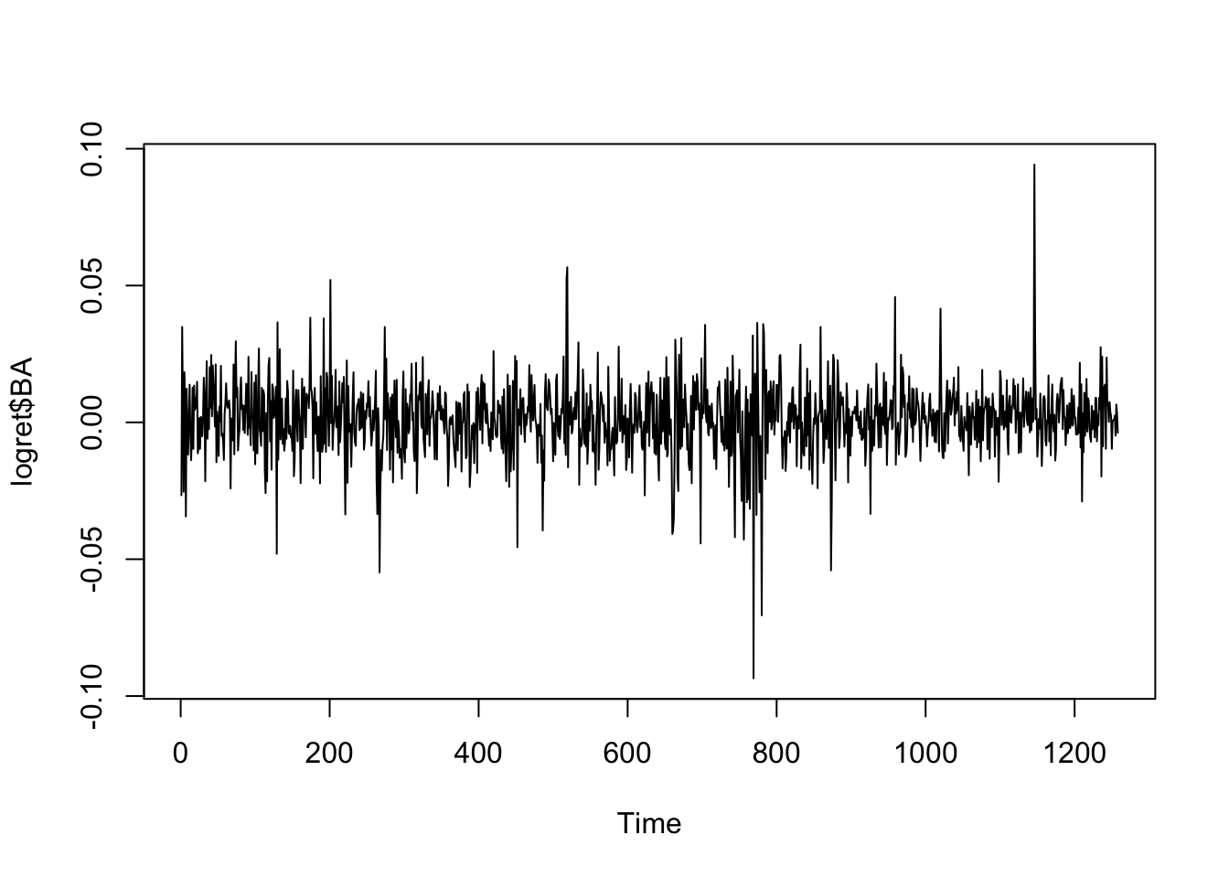
The aim is to study the temporal correlation and the auto-dependence in time. We will make use of the function lag.plot which plots a time-series against lagged versions of themselves. This concept is also explained in Figure 12.1 which refers to a simple case with \(n=6\) observations. It is important to note that when the lag \(h\) increases the number of observations (couples) used to compute the auto-correlation decreases. Thus, the maximum value of \(h\) that can be considered is \(n-1\). However, this is not a problem for us as we usually work with very long time series.
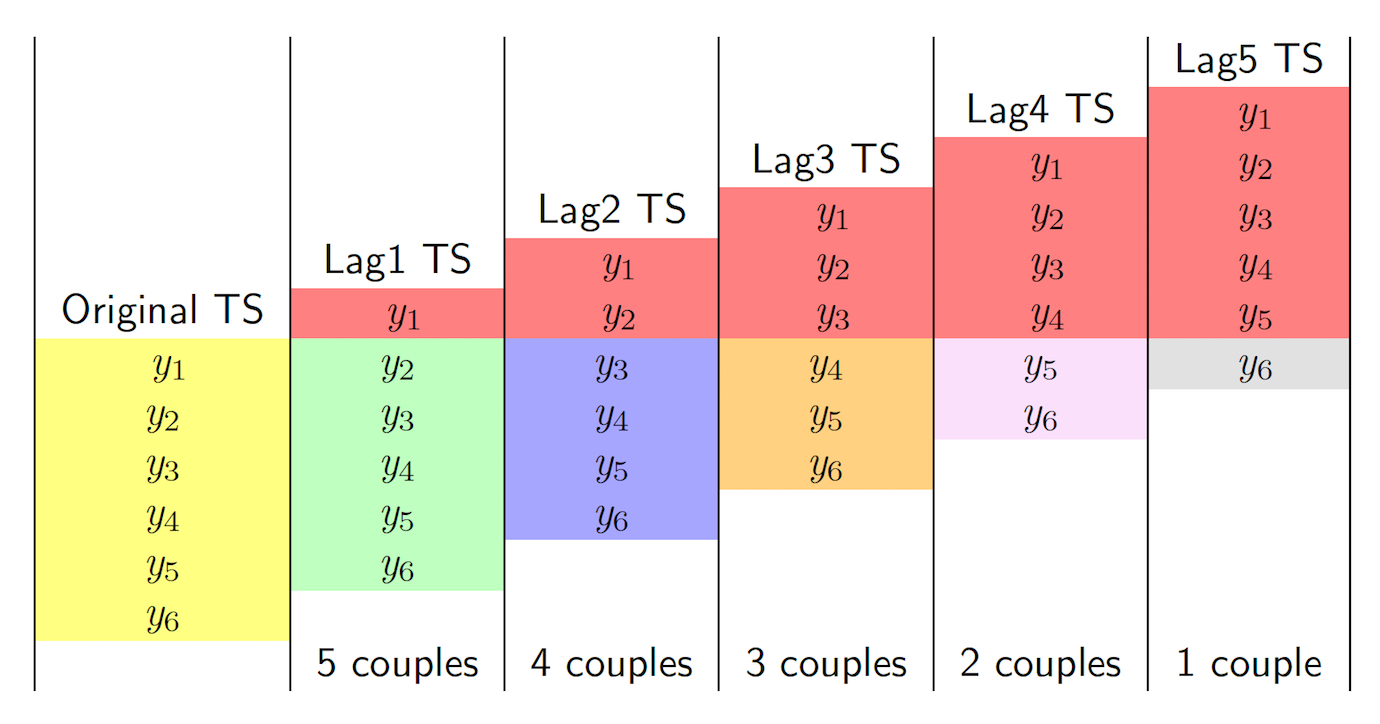
Figure 12.1: How auto-correlation is computed: the case with \(n=6\) observations
The following code produces the scatterplot of the couples with distance (lag) equal to one day (i.e. \(y_t\) vs \(y_{t-1}\) for all \(t=2,3, \ldots,\) 1258).
lag.plot(logret$BA, set.lags = 1) #h=1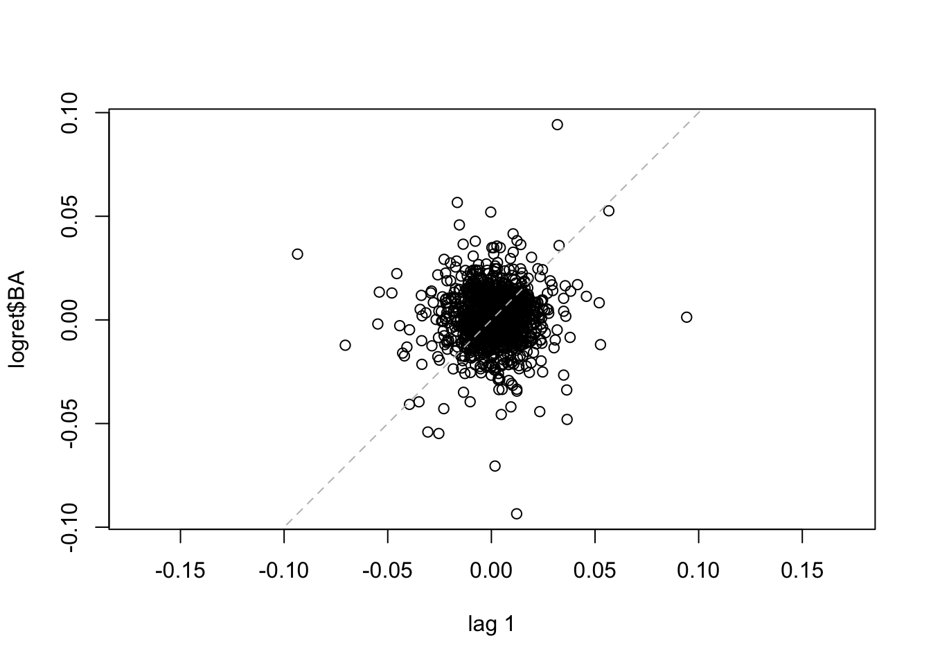 The dashed line in the plot is the bisector. We observe that the points are spread all across the plot denoting a weak correlation. The same plot can be obtained for \(h=2\) (for plotting \(y_t\) vs \(y_{t-2}\) for all \(t=3, \ldots,\) 1258) ), 500 and 1000.
lag.plot(logret$BA, set.lags = 2) #h=2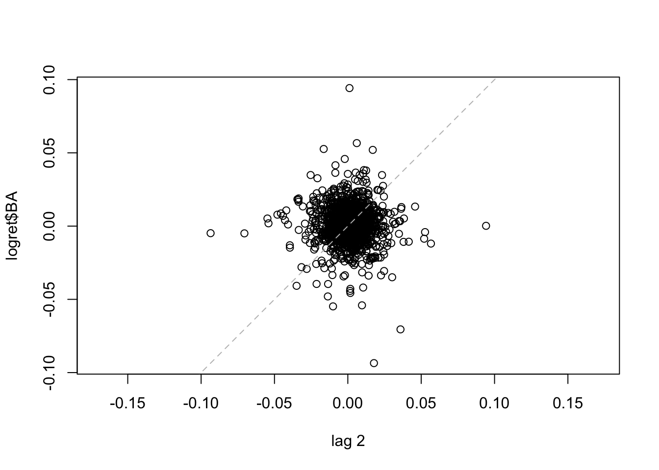
lag.plot(logret$BA, set.lags = 500) #h=500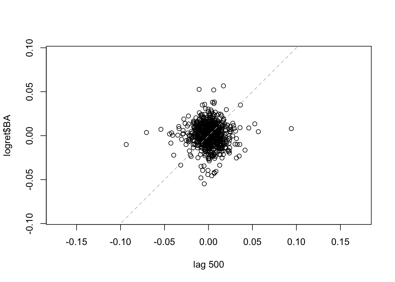
lag.plot(logret$BA, set.lags = 1000) #h=1000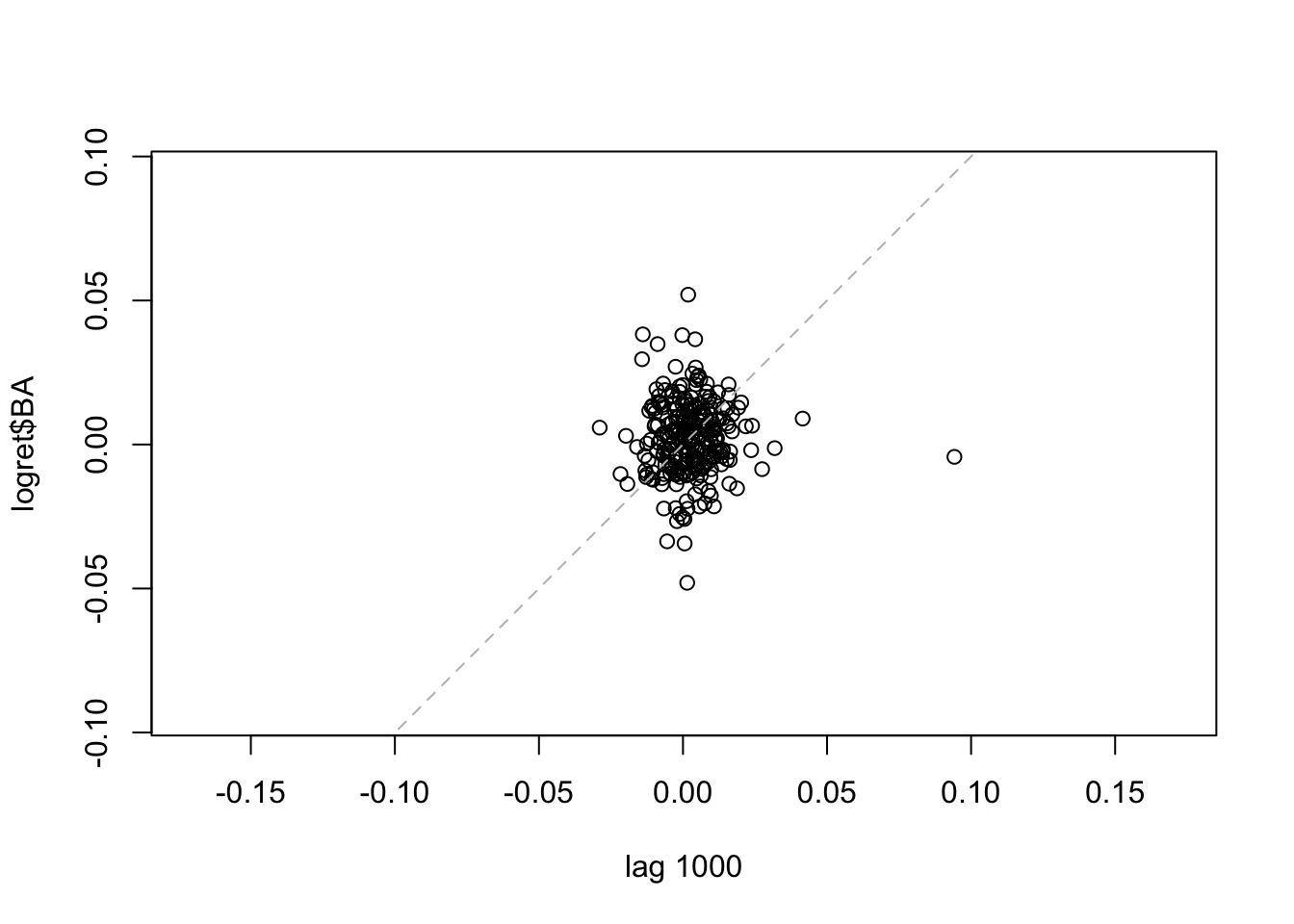 We note that for the considered lags the correlation is always weak. It is worth to note that the number of points is smaller for high values of \(h\). It is also possible to consider more lags jointly:
lag.plot(logret$BA, set.lags = 1:10) 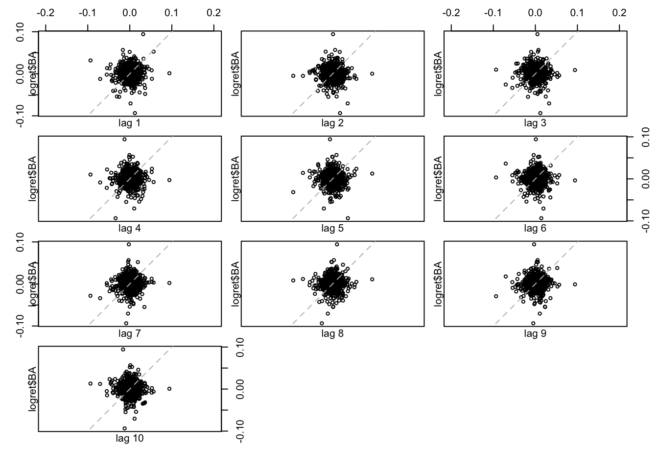 All the 10 plots show a very weak (auto)-correlation. To quantify it we can compute the values of the auto-correlation function by using the
 acf function:
acf(logret$BA, plot=FALSE)##
## Autocorrelations of series 'logret$BA', by lag
##
## 0 1 2 3 4 5 6 7 8 9 10
## 1.000 0.033 -0.032 0.006 0.005 -0.051 -0.008 0.012 0.019 0.026 -0.046
## 11 12 13 14 15 16 17 18 19 20 21
## 0.022 0.017 -0.012 -0.008 -0.031 0.037 0.013 0.005 -0.010 0.022 0.003
## 22 23 24 25 26 27 28 29 30
## 0.025 0.015 0.048 0.032 -0.002 -0.002 -0.016 0.024 0.013It can be observed that all the values of the auto-correlation, for lags between 1 and 30. The considered maximum lag is given by \(10 \times log 10 \times n\) where \(n\) is the time series length (this can be changed with the lag.max argument).
The plot of the auto-correlation function, known as correlogram, can be obtained by using the same function acf with the option plot=TRUE. As the latter is the default specification we will omit it.
acf(logret$BA)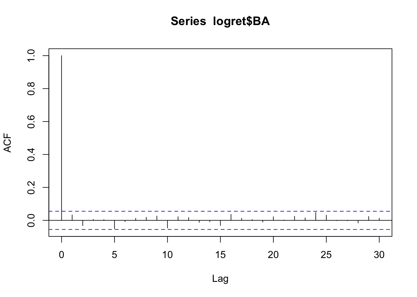 All the vertical bars are contained between the blue lines. This means that there are no significant correlations. These data could have been generated by a white-noise with uncorrelated components. Can we conclude that we have also independent components (remember that in general uncorrelation does not imply independence)? To check this we take into account a transformation of the data (e.g. square or absolute value transformation).
acf(logret$BA^2)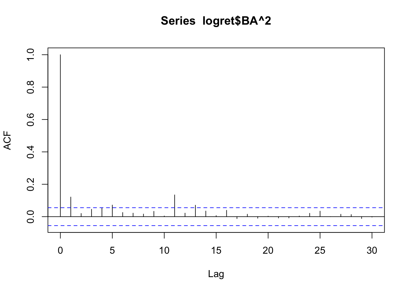
acf(abs(logret$BA))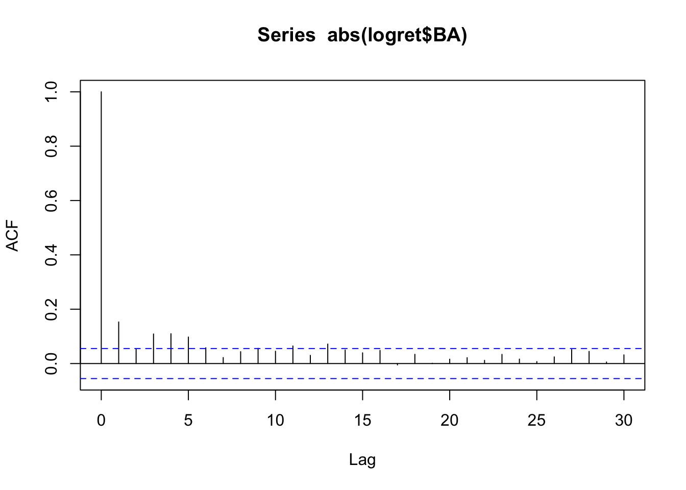 We see some significant correlations and so we conclude that we don’t have independence (if the data were independent, we would see no significant correlations in the correlogram of the transformed data).
12.1.1 lag.plot for dependent sequences
Let’s see the kind of lag.plot we obtain for an auto-correlated sequence. In the following chunk I simulate a time series from an AR\((1)\) process.
sim_data<- arima.sim(n=1000,model=list(ar=0.6,ma=0))As we expect the sequence is stationary and auto-correlated, as we can deduce from the following plot:
par(mfrow=c(1,2))
ts.plot(sim_data)
acf(sim_data)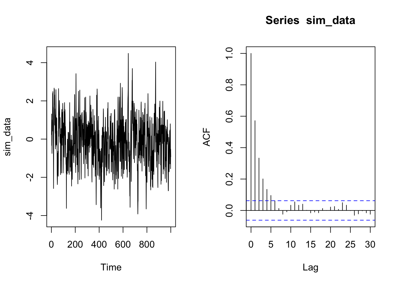
Let’s give a look at the lag.plot for lag \(h\) equal to \(1,2,\dots,10\)
lag.plot(sim_data, set.lags = 1:10) 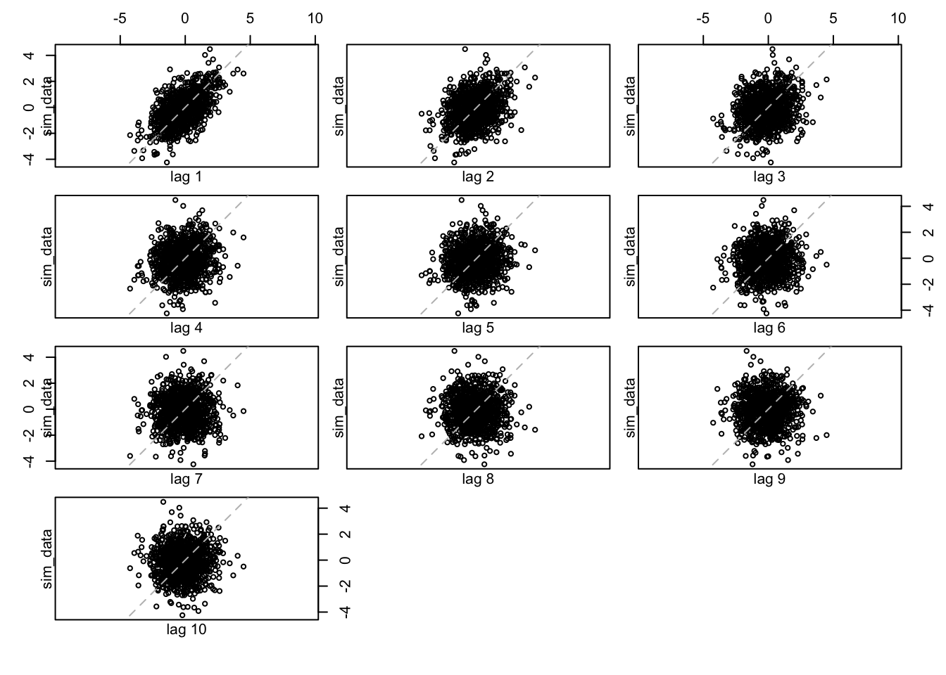
We can notice how the autocorrelation decreases and it disappear starting at lag equal to \(5\).
12.2 Ljung-Box test
We consider now a different time series for the CSCO asset.
ts.plot(logret$CSCO)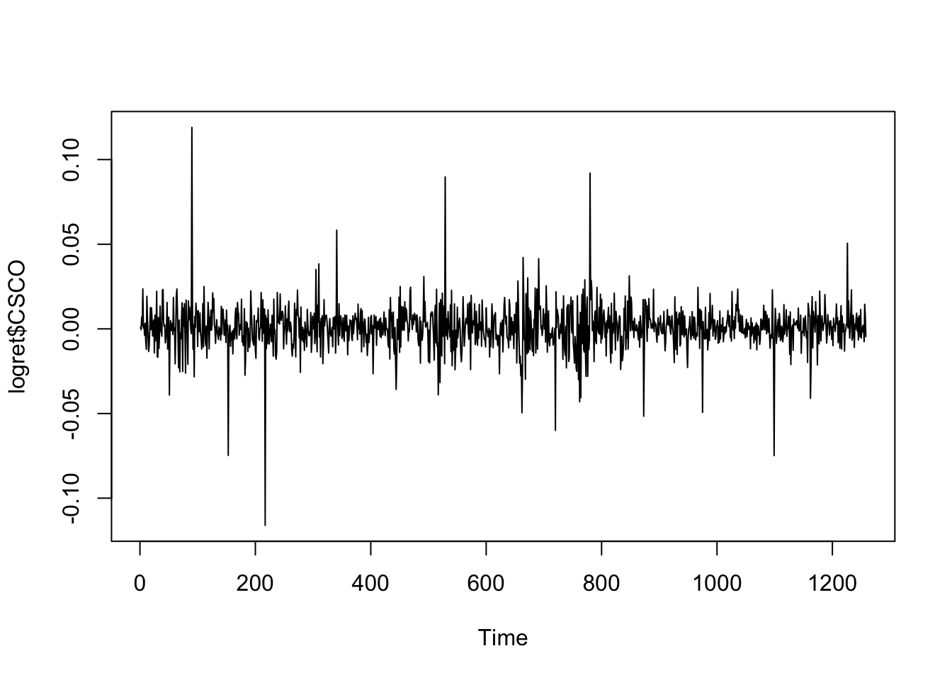
acf(logret$CSCO)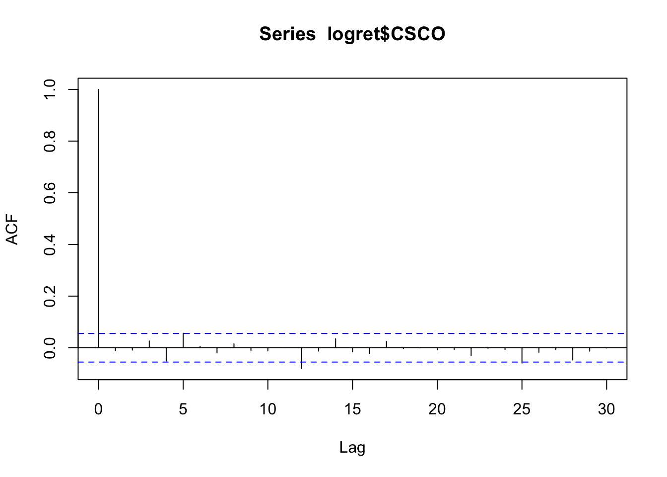 We note that all the correlations except for \(h=12\) are not significant (the bars are inside the blue lines and we do not reject the null hypothesis \(H_0:\rho(h)=0\)). Is the case of \(h=12\) a false positive or a real significant correlation? To check this we can use the simultaneous Ljung-Box test implemented in R by using the function
 Box.test (see ?Box.test), where we set lag=12 because we want to test \(H_0: \rho(1)=\rho(2)=\ldots=\rho(12)=0\). It is also necessary to specify the test we want to implement with type="L". In this case the test statistic is distributed as \(\chi^2_{12}\).
Box.test(logret$CSCO,lag=12,type="L")##
## Box-Ljung test
##
## data: logret$CSCO
## X-squared = 17.969, df = 12, p-value = 0.1166Given the p-value, we do not reject the null hypothesis and thus we can considered that there is no significant correlation at any lag for the considered data.
12.3 Looking for stationarity
We import now the GNP data. They refer to the series of US Gross National Product (GNP) in Billions of Dollars (seasonally Adjusted Annual Rate, quarterly frequency from January 1947 to July 2017).
GNPdf <- read.csv("files/GNP.csv")
str(GNPdf)
## 'data.frame': 283 obs. of 2 variables:
## $ DATE: chr "1947-01-01" "1947-04-01" "1947-07-01" "1947-10-01" ...
## $ GNP : num 244 247 251 262 268 ...head(GNPdf)## DATE GNP
## 1 1947-01-01 244.058
## 2 1947-04-01 247.362
## 3 1947-07-01 251.246
## 4 1947-10-01 261.545
## 5 1948-01-01 267.564
## 6 1948-04-01 274.376tail(GNPdf)## DATE GNP
## 278 2016-04-01 18733.02
## 279 2016-07-01 18917.47
## 280 2016-10-01 19134.46
## 281 2017-01-01 19271.96
## 282 2017-04-01 19452.41
## 283 2017-07-01 19722.06The time series is characterized by an increasing momentum and thus it is not stationary:
ts.plot(GNPdf$GNP)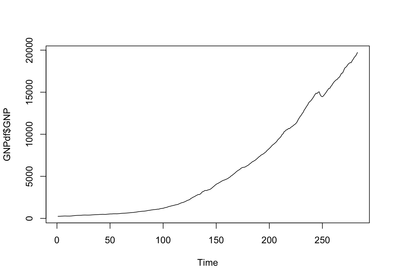
We thus try to compute the first order difference by using the diff function:
ts.plot(diff(GNPdf$GNP))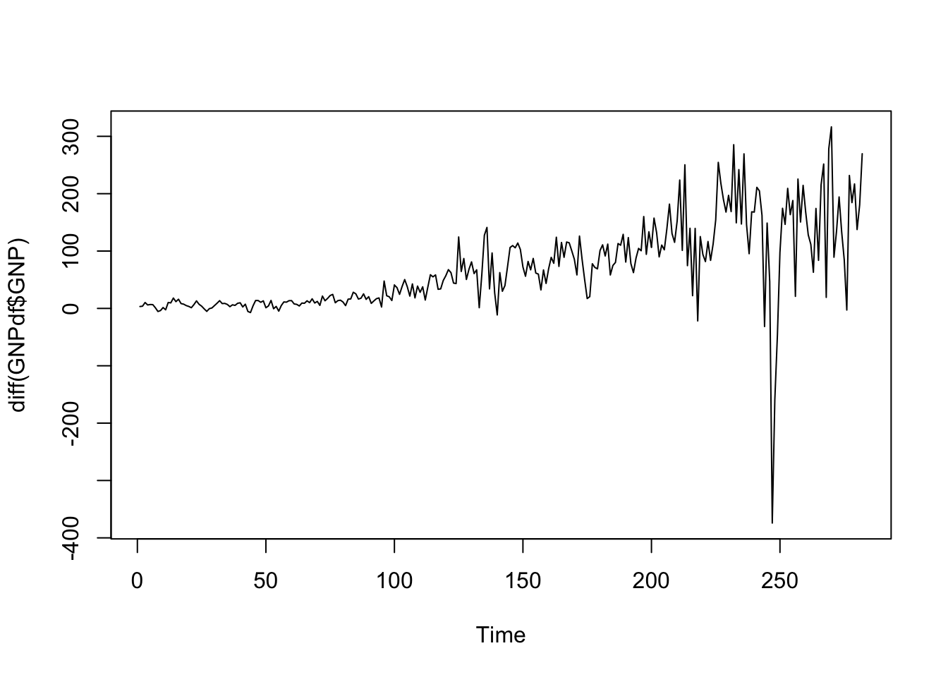 The situation is still non stationary as it seems characterized by different values of mean and variance. We proceed by differencing one more time by applying the
 diff function twice:
ts.plot(diff(diff(GNPdf$GNP)))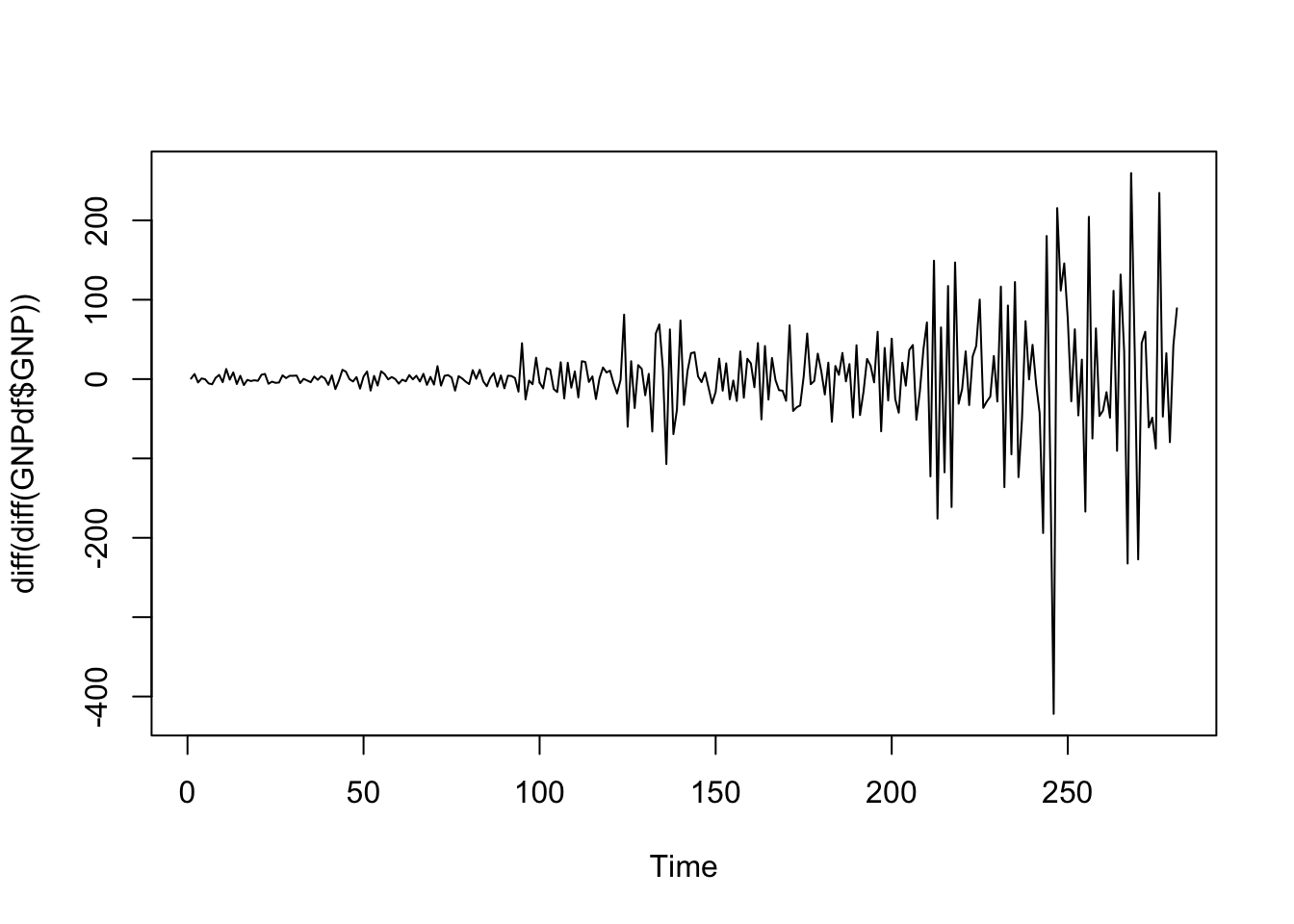 The time series now seems to revert to zero but the variability increases in time. This can be fixed by applying a transformation of the data that stabilizes the variance. We consider the log transformation which belongs to the Box-Cox family of transformations. Logs are useful because they are nice interpretation:
changes in a log value corresponds to relative (percent) changes on the original scale.
The time series now seems to revert to zero but the variability increases in time. This can be fixed by applying a transformation of the data that stabilizes the variance. We consider the log transformation which belongs to the Box-Cox family of transformations. Logs are useful because they are nice interpretation:
changes in a log value corresponds to relative (percent) changes on the original scale.
We add the transformed data in the dataframe
GNPdf$logGNP = log(GNPdf$GNP)
ts.plot(GNPdf$logGNP)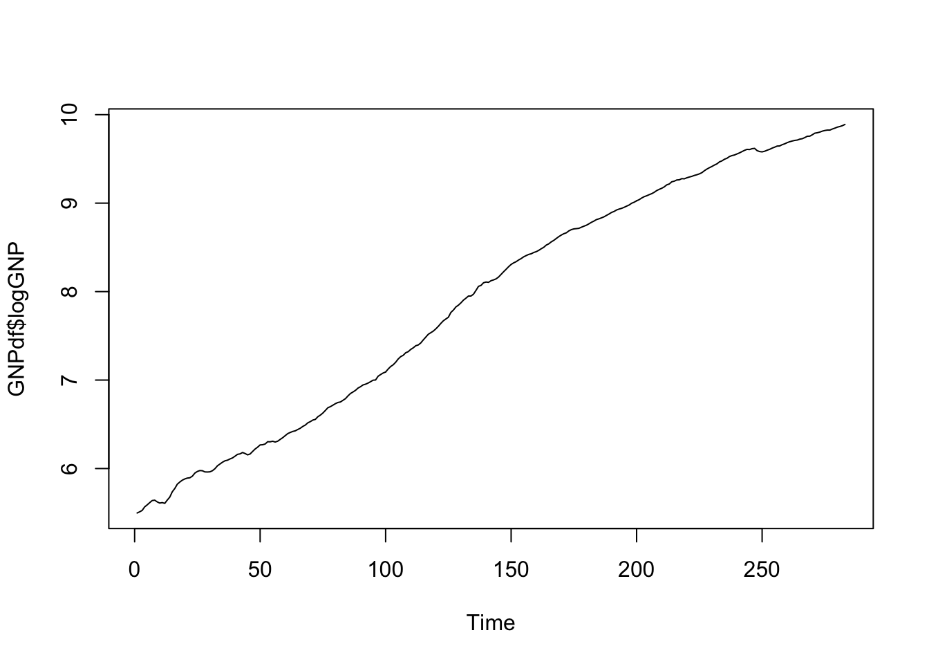 and then compute again differences:
ts.plot(diff(GNPdf$logGNP))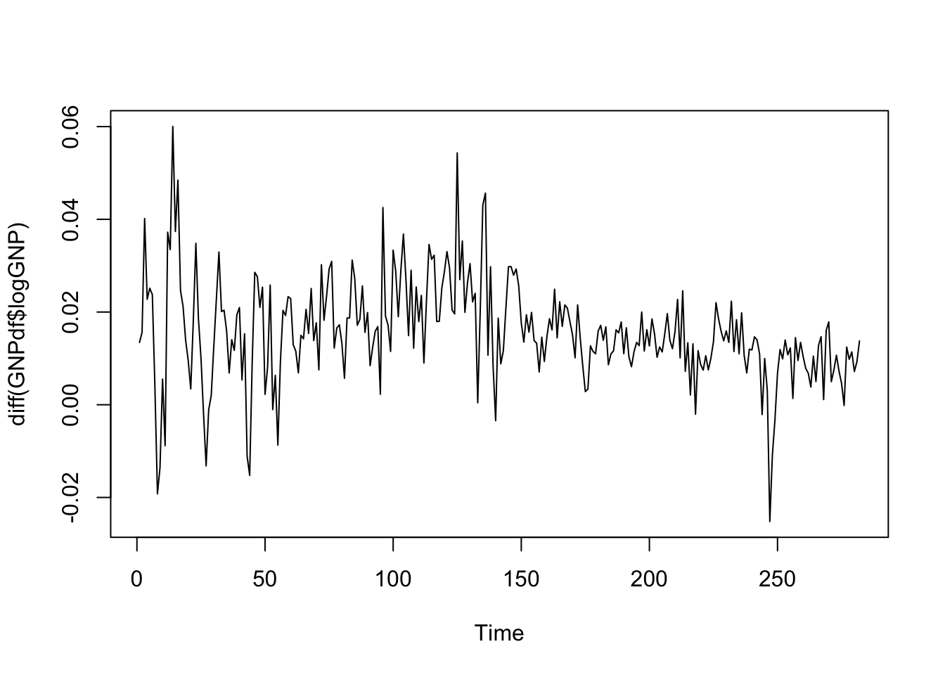
ts.plot(diff(diff(GNPdf$logGNP)))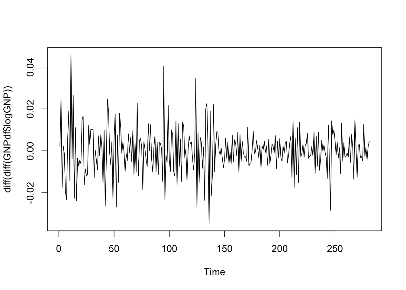 The time series of the second order differences of log GNP values seems to be mean reverting. We are maybe not so sure about variability which seems higher at the beginning of the period. In this case it is possible to use the Augmented Dickey Fuller test to verify stationarity (link). The function
 adf.test is included in the tseries package. It tests the null hypothesis of a unit root (i.e. non stationarity) vs the alternative hypothesis of stationary or explosive process.
logGNP2 = diff(diff(GNPdf$logGNP))
library(tseries)
adf.test(logGNP2, alternative = "stationary")
## Warning in adf.test(logGNP2, alternative = "stationary"): p-value smaller than
## printed p-value##
## Augmented Dickey-Fuller Test
##
## data: logGNP2
## Dickey-Fuller = -10.505, Lag order = 6, p-value = 0.01
## alternative hypothesis: stationaryGiven the p-value, we reject H0 and we accept the stationarity hypothesis for the logGNP2 time series. We thus go on with the analysis, by analysing the auto-correlation (acf) and the partial auto-correlation function (pacf):
acf(logGNP2) 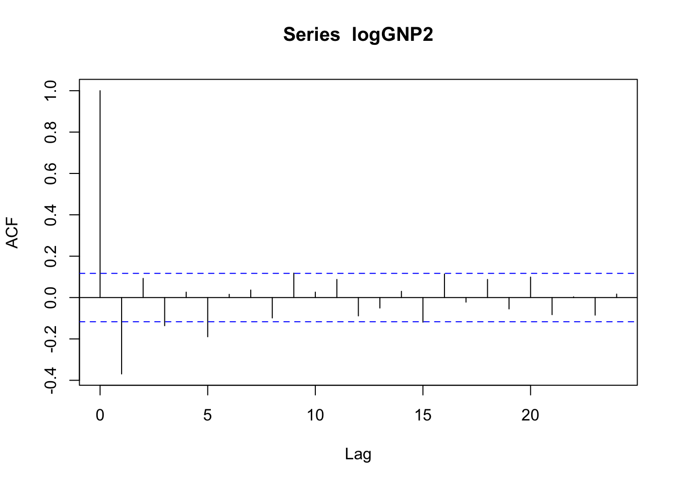
pacf(logGNP2)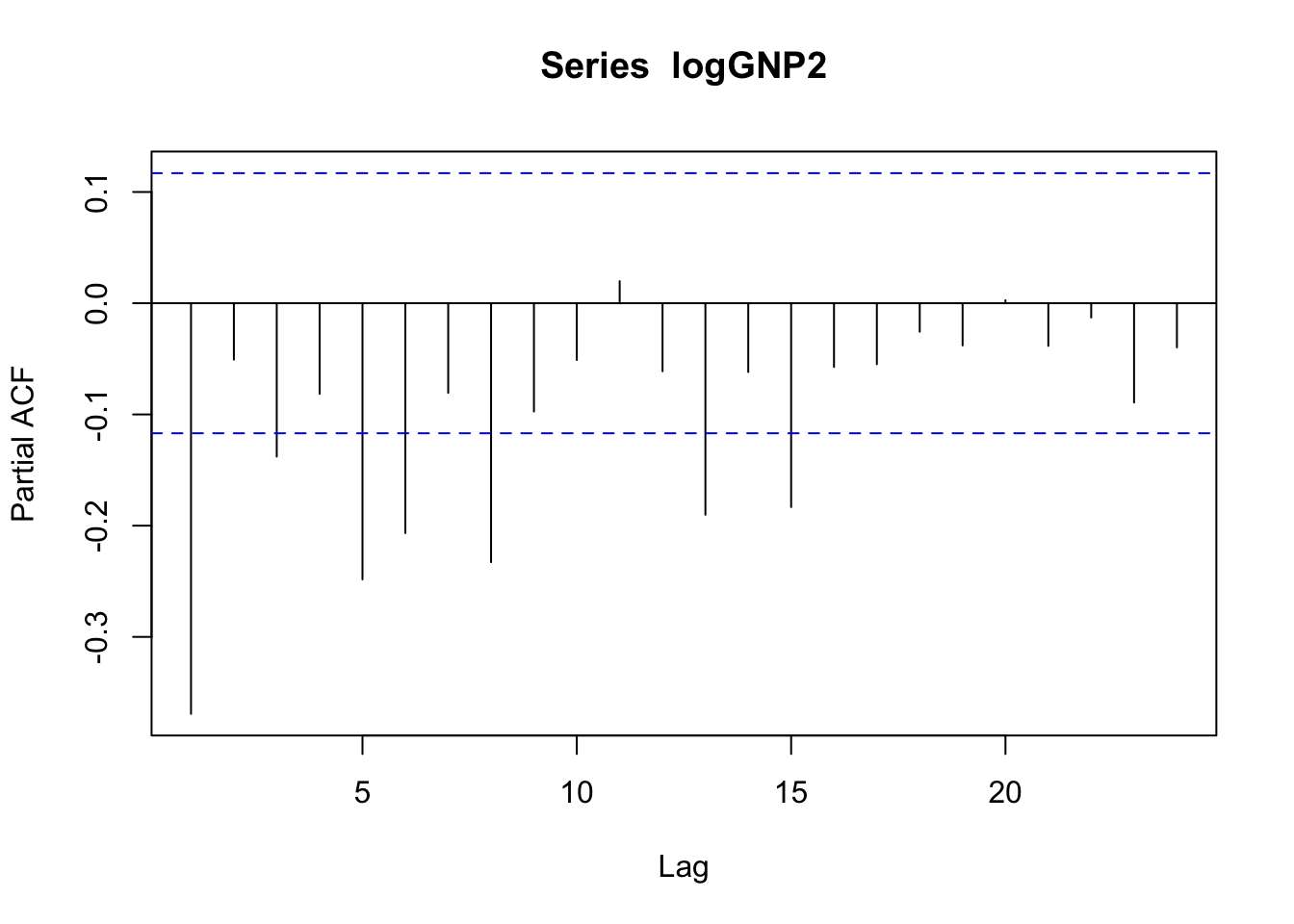 The temporal pattern is not clear neither for the correlogram (is it a cut-off at lag 5?) nor the pacf plot (is it a tail-off with wave pattern?). We will different ARMA models and choose the best one according to residuals analysis and the AIC index value.
12.4 Estimate ARIMA models
We will start by estimating a MA(1) model. We will use the Arima function which is part of the forecast package. It is known that the Arima function adopts maximum likelihood for estimation; thus, the coefficients are asymptotically normally distributed. Hence, if you the divide each coefficient by its standard error you get the corresponding z-statistic value and it is then possible to compute the p-value to test if the parameter is significantly different from zero.
For estimating a model, we have to specify the data and the order \((p,d,q)\) of the model. Also the option include.constant=TRUE has to be included.
library(forecast)
mod1 = Arima(logGNP2, order=c(0,0,1),
             include.constant = TRUE)
summary(mod1)
## Series: logGNP2
## ARIMA(0,0,1) with non-zero mean
##
## Coefficients:
## ma1 mean
## -0.4883 0e+00
## s.e. 0.0833 3e-04
##
## sigma^2 estimated as 0.0001035: log likelihood=891.38
## AIC=-1776.76 AICc=-1776.67 BIC=-1765.84
##
## Training set error measures:
## ME RMSE MAE MPE MAPE MASE
## Training set 2.427488e-05 0.01013676 0.00741686 205.2358 351.3944 0.5454505
## ACF1
## Training set 0.05841076The parameter estimates can be retrieved with
mod1$coef## ma1 intercept
## -4.883294e-01 -2.360583e-05The estimated model is given by \(Y_t=\epsilon_t\)-0.488\(\epsilon_{t-1}\) (mean is omitted as it is very small). We are interested in the analysis of the model residuals in order to see if there is still some temporal correlation. We can use the checkresiduals function which provides some plots for the residuals (including the correlogram) and the Ljung-Box test output.
checkresiduals(mod1)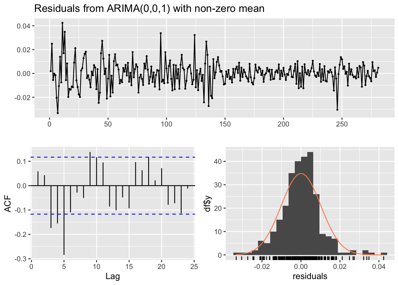
##
##  Ljung-Box test
##
## data:  Residuals from ARIMA(0,0,1) with non-zero mean
## Q* = 54.359, df = 8, p-value = 5.881e-09
##
## Model df: 2.   Total lags used: 10
Note that in the Ljung-Box test the number of considered lags is 10 (we are checking if the first 10 correlations are equal to zero); if necessary this can be changed by using the lag argument. Moreover, the number of model degrees of freedom is 2 (given by the number of parameters estimated, \(\mu\) and \(\theta\)) and the number of degrees of freedom of the \(\chi^2\) distribution is 8 (the number of estimated parameters can be set also manually with the df argument). Remember that if you want to use the Box.test function for the residuals you have to specify with the argument fitdf the number of estimated parameters. Given the p-value we reject the simultaneous uncorrelation hypothesis (this is confirmed also by the correlogram). It means that the MA(1) is not enough for catching the temporal structure of the data. Let’s consider the AR(1) model.
mod2 = Arima(logGNP2, order=c(1,0,0),
             include.constant = TRUE)
summary(mod2)
## Series: logGNP2
## ARIMA(1,0,0) with non-zero mean
##
## Coefficients:
## ar1 mean
## -0.3682 0e+00
## s.e. 0.0553 5e-04
##
## sigma^2 estimated as 0.0001056: log likelihood=888.55
## AIC=-1771.09 AICc=-1771.01 BIC=-1760.18
##
## Training set error measures:
## ME RMSE MAE MPE MAPE MASE
## Training set 2.368045e-06 0.01024175 0.007489712 198.4469 319.9212 0.5508082
## ACF1
## Training set -0.02013451checkresiduals(mod2)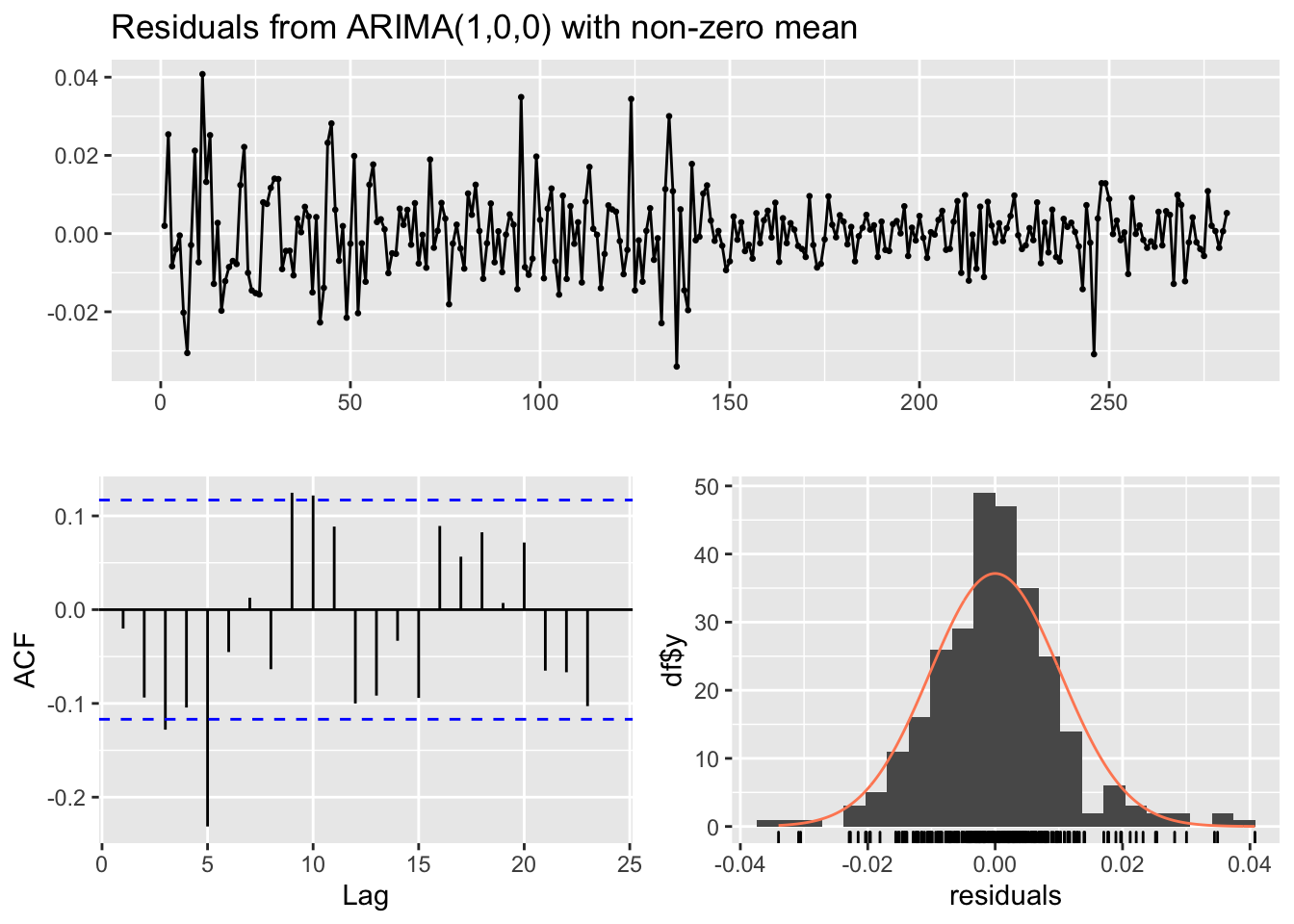
##
##  Ljung-Box test
##
## data:  Residuals from ARIMA(1,0,0) with non-zero mean
## Q* = 36.551, df = 8, p-value = 1.392e-05
##
## Model df: 2.   Total lags used: 10
The estimated model is \(Y_t =\)-0.368\(Y_{t-1}+\epsilon_t\).
Also the performance of the AR(1) is poor as there is still some correlation in the residuals. In any case, we can compare mod1 and mod2 by using the AIC:
mod1$aic## [1] -1776.756mod2$aic## [1] -1771.092We observe that mod1 should be preferred. In the following we will try many other different models: # ARMA(1,1), ARMA(2,1), ARMA(2,2), ARMA(3,1), ARMA(1,3), ARMA(2,3) and ARMA(3,2).
######### ARMA(1,1) #########
mod3 = Arima(logGNP2, order=c(1,0,1),
             include.constant = TRUE)
summary(mod3)
## Series: logGNP2
## ARIMA(1,0,1) with non-zero mean
##
## Coefficients:
## ar1 ma1 mean
## 0.4161 -0.9623 0e+00
## s.e. 0.0589 0.0177 1e-04
##
## sigma^2 estimated as 9.006e-05: log likelihood=910.67
## AIC=-1813.33 AICc=-1813.19 BIC=-1798.78
##
## Training set error measures:
## ME RMSE MAE MPE MAPE MASE
## Training set 4.807754e-06 0.009439138 0.006820991 175.5431 236.4172 0.5016291
## ACF1
## Training set -0.04671616checkresiduals(mod3)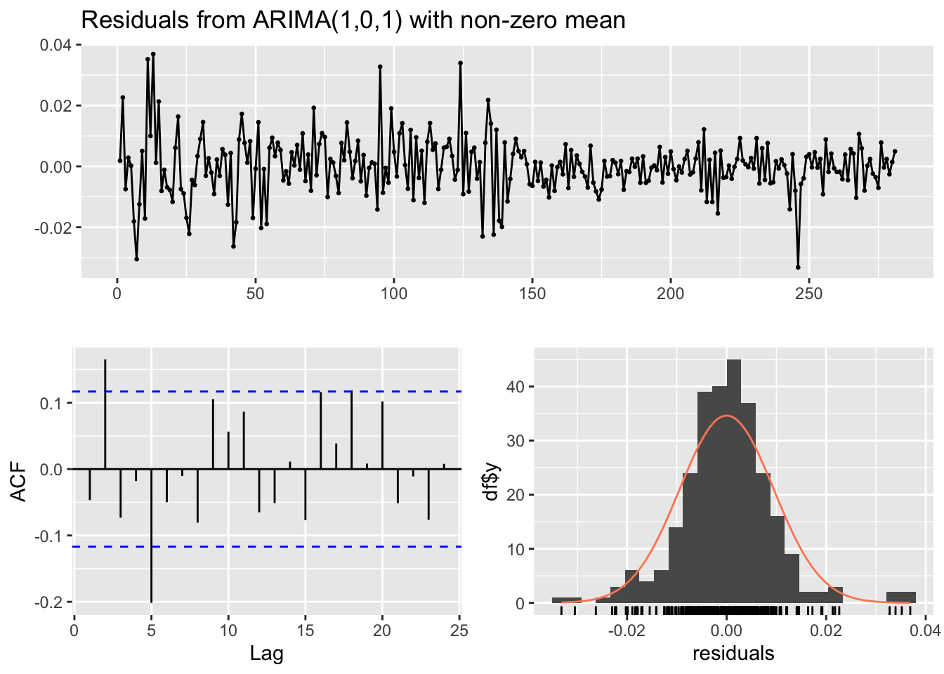
##
##  Ljung-Box test
##
## data:  Residuals from ARIMA(1,0,1) with non-zero mean
## Q* = 28.586, df = 7, p-value = 0.0001721
##
## Model df: 3.   Total lags used: 10
######### ARMA(2,1) #########
mod4 = Arima(logGNP2, order=c(2,0,1),
include.constant = TRUE)
summary(mod4)## Series: logGNP2
## ARIMA(2,0,1) with non-zero mean
##
## Coefficients:
## ar1 ar2 ma1 mean
## 0.3780 0.1184 -0.9706 0e+00
## s.e. 0.0618 0.0614 0.0176 1e-04
##
## sigma^2 estimated as 8.919e-05: log likelihood=912.53
## AIC=-1815.06 AICc=-1814.84 BIC=-1796.87
##
## Training set error measures:
## ME RMSE MAE MPE MAPE MASE
## Training set 2.931111e-05 0.009376612 0.006751608 207.9673 287.0736 0.4965266
## ACF1
## Training set 0.01841865checkresiduals(mod4)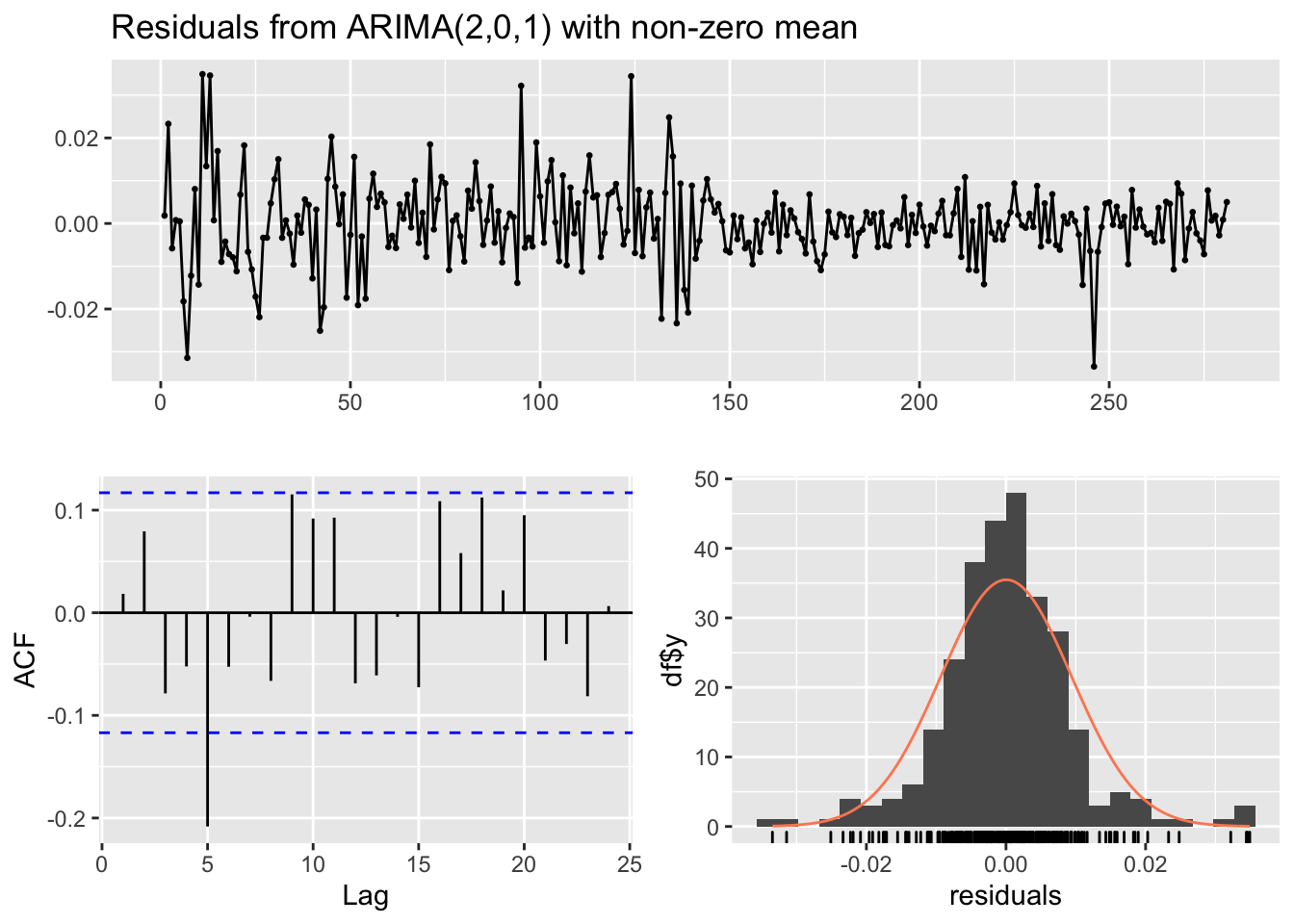
##
##  Ljung-Box test
##
## data:  Residuals from ARIMA(2,0,1) with non-zero mean
## Q* = 25.384, df = 6, p-value = 0.0002898
##
## Model df: 4.   Total lags used: 10
######### ARMA(2,2) #########
mod5 = Arima(logGNP2, order=c(2,0,2),
include.constant = TRUE)
summary(mod5)## Series: logGNP2
## ARIMA(2,0,2) with non-zero mean
##
## Coefficients:
## ar1 ar2 ma1 ma2 mean
## -0.1836 0.3745 -0.4025 -0.5486 0e+00
## s.e. 0.1762 0.0787 0.1798 0.1712 1e-04
##
## sigma^2 estimated as 8.815e-05: log likelihood=914.67
## AIC=-1817.33 AICc=-1817.02 BIC=-1795.5
##
## Training set error measures:
## ME RMSE MAE MPE MAPE MASE
## Training set 2.827708e-05 0.009305174 0.006668397 213.8634 291.7492 0.490407
## ACF1
## Training set 0.0150511checkresiduals(mod5)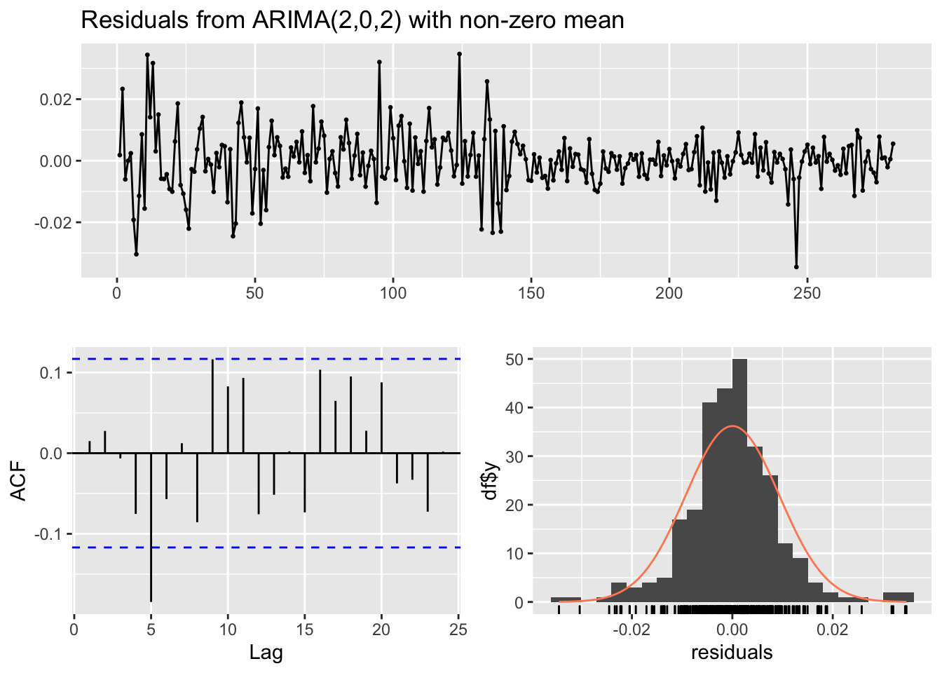
##
##  Ljung-Box test
##
## data:  Residuals from ARIMA(2,0,2) with non-zero mean
## Q* = 20.823, df = 5, p-value = 0.0008749
##
## Model df: 5.   Total lags used: 10
######### ARMA(3,1) #########
mod6 = Arima(logGNP2, order=c(3,0,1),
include.constant = TRUE)
summary(mod6)## Series: logGNP2
## ARIMA(3,0,1) with non-zero mean
##
## Coefficients:
## ar1 ar2 ar3 ma1 mean
## 0.3852 0.1708 -0.1725 -0.9577 0e+00
## s.e. 0.0606 0.0630 0.0607 0.0191 1e-04
##
## sigma^2 estimated as 8.702e-05: log likelihood=916.46
## AIC=-1820.93 AICc=-1820.62 BIC=-1799.1
##
## Training set error measures:
## ME RMSE MAE MPE MAPE MASE
## Training set 1.783105e-05 0.009245019 0.006574007 186.7293 252.9048 0.4834654
## ACF1
## Training set -0.01776276checkresiduals(mod6)
##
##  Ljung-Box test
##
## data:  Residuals from ARIMA(3,0,1) with non-zero mean
## Q* = 17.037, df = 5, p-value = 0.00443
##
## Model df: 5.   Total lags used: 10
######### ARMA(1,3) #########
mod7 = Arima(logGNP2, order=c(1,0,3),
include.constant = TRUE)
summary(mod7)## Series: logGNP2
## ARIMA(1,0,3) with non-zero mean
##
## Coefficients:
## ar1 ma1 ma2 ma3 mean
## 0.3332 -0.9211 0.1555 -0.1929 0e+00
## s.e. 0.1530 0.1532 0.1304 0.0652 1e-04
##
## sigma^2 estimated as 8.787e-05: log likelihood=915.13
## AIC=-1818.25 AICc=-1817.95 BIC=-1796.42
##
## Training set error measures:
## ME RMSE MAE MPE MAPE MASE
## Training set 2.647367e-05 0.009289874 0.006652528 211.2842 281.9028 0.48924
## ACF1
## Training set 0.003535468checkresiduals(mod7)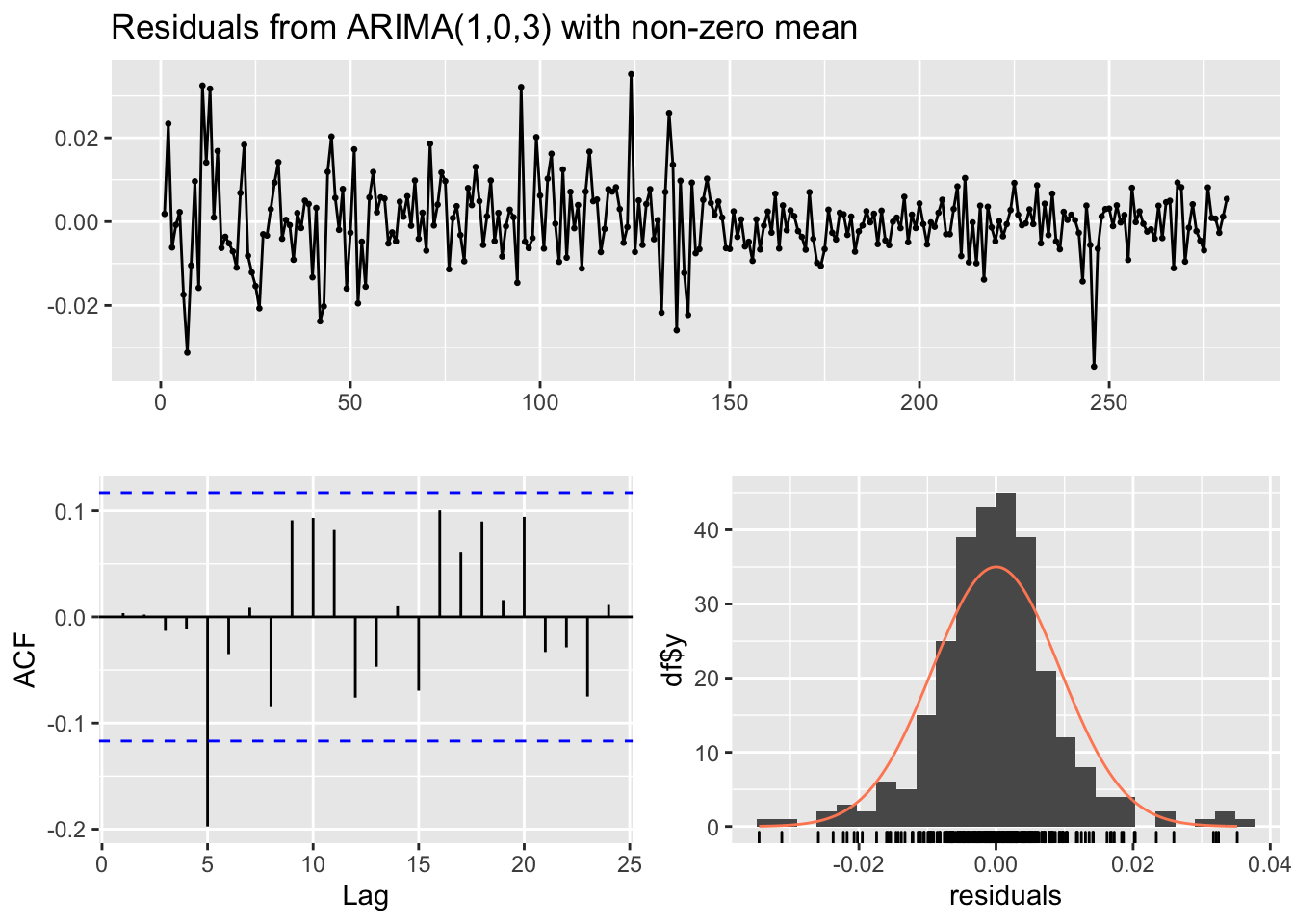
##
##  Ljung-Box test
##
## data:  Residuals from ARIMA(1,0,3) with non-zero mean
## Q* = 18.776, df = 5, p-value = 0.002116
##
## Model df: 5.   Total lags used: 10
######### ARMA(2,3) #########
mod8 = Arima(logGNP2, order=c(2,0,3),
include.constant = TRUE)
summary(mod8)## Series: logGNP2
## ARIMA(2,0,3) with non-zero mean
##
## Coefficients:
## ar1 ar2 ma1 ma2 ma3 mean
## -0.1879 0.2820 -0.3862 -0.4622 -0.0948 0e+00
## s.e. 0.2221 0.1359 0.2277 0.2297 0.1023 1e-04
##
## sigma^2 estimated as 8.822e-05: log likelihood=915.07
## AIC=-1816.13 AICc=-1815.72 BIC=-1790.66
##
## Training set error measures:
## ME RMSE MAE MPE MAPE MASE
## Training set 2.382653e-05 0.009291752 0.006647268 200.0394 277.0012 0.4888531
## ACF1
## Training set -0.0003539481checkresiduals(mod8)
##
##  Ljung-Box test
##
## data:  Residuals from ARIMA(2,0,3) with non-zero mean
## Q* = 19.605, df = 4, p-value = 0.0005974
##
## Model df: 6.   Total lags used: 10
######### ARMA(3,2) #########
mod9 = Arima(logGNP2, order=c(3,0,2),
include.constant = TRUE)
summary(mod9)## Series: logGNP2
## ARIMA(3,0,2) with non-zero mean
##
## Coefficients:
## ar1 ar2 ar3 ma1 ma2 mean
## 1.0208 -0.0725 -0.2551 -1.6275 0.6548 0e+00
## s.e. 0.1686 0.1105 0.0613 0.1718 0.1652 1e-04
##
## sigma^2 estimated as 8.514e-05: log likelihood=919.95
## AIC=-1825.89 AICc=-1825.48 BIC=-1800.43
##
## Training set error measures:
## ME RMSE MAE MPE MAPE MASE
## Training set 4.601698e-05 0.009128333 0.006474332 139.5792 223.9337 0.4761351
## ACF1
## Training set -0.003316259checkresiduals(mod9)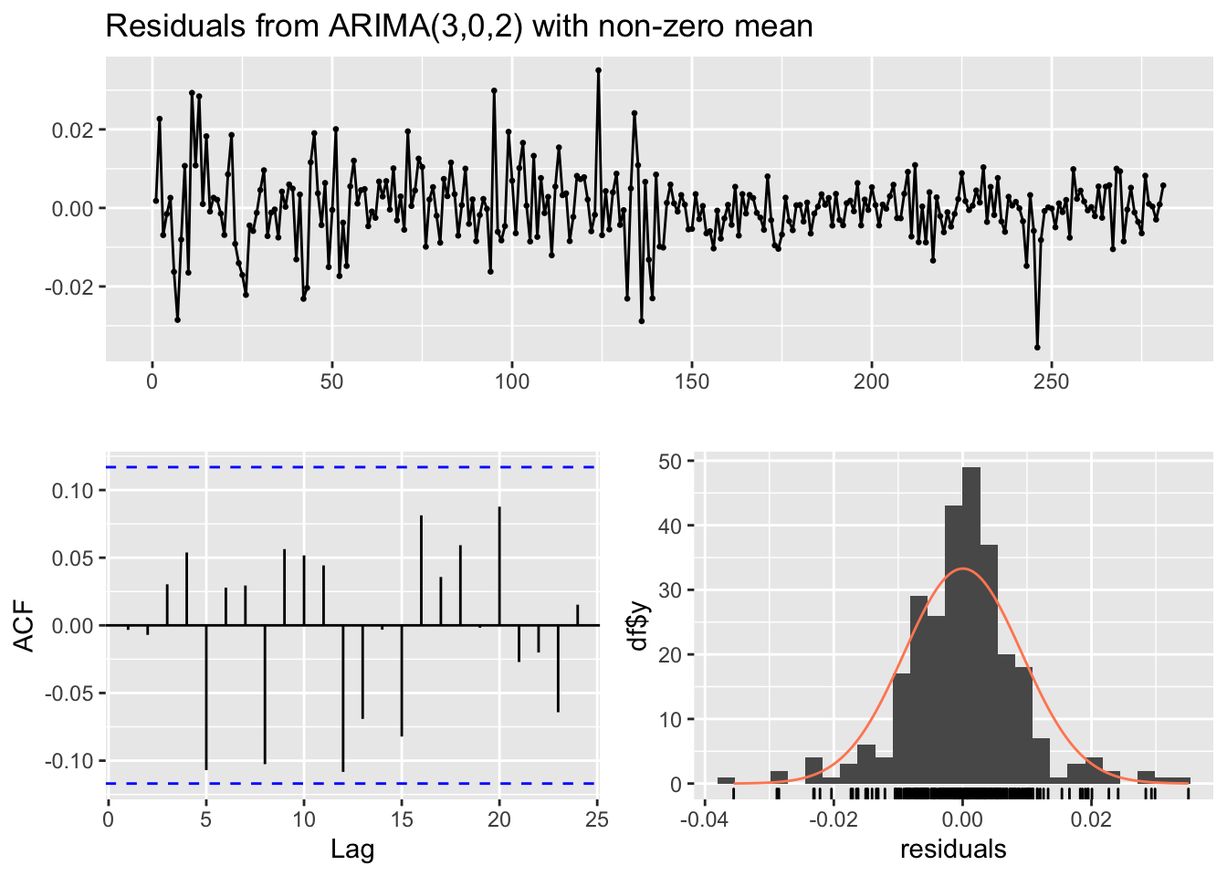
##
##  Ljung-Box test
##
## data:  Residuals from ARIMA(3,0,2) with non-zero mean
## Q* = 9.666, df = 4, p-value = 0.04645
##
## Model df: 6.   Total lags used: 10
all_aic = c(mod1$aic, mod2$aic, mod3$aic, mod4$aic,mod5$aic, mod6$aic, mod7$aic, mod8$aic,mod9$aic)
min(all_aic)## [1] -1825.894which.min(all_aic)## [1] 9The model with the lowest AIC is mod9 (ARMA(3,2)). Moreover, its residuals are uncorrelated, meaning that there is no residual correlation is left. The corresponding estimated model equation is $Y_t=$1.021 \(Y_{t-1}\) -0.073 \(Y_{t-2}\) -0.255 \(Y_{t-3}+\epsilon_t\) -1.628 \(\epsilon_{t-1}\) +0.655 \(\epsilon_{t-2}\).
Once we have chosen the best model we can plot observed and fitted values:
ts.plot(logGNP2, col="grey")
lines(mod9$fitted, col="blue")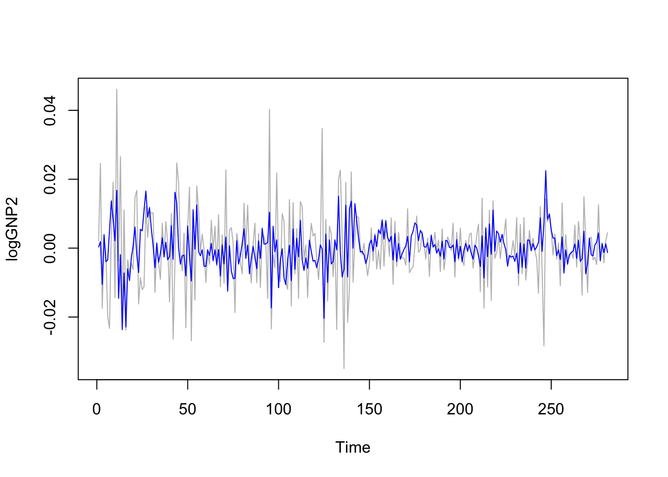 We observe that model is not able to pick the extreme values of the series. We proceed now with forecasting, i.e. the prediction of the time series values for the following 10 days. To do this we use the
 forecast function:
forecast(mod9)## Point Forecast Lo 80 Hi 80 Lo 95 Hi 95
## 282 -3.297003e-03 -0.01512236 0.008528357 -0.02138233 0.01478832
## 283 -4.933976e-04 -0.01432511 0.013338316 -0.02164718 0.02066038
## 284 -1.407692e-03 -0.01524636 0.012430972 -0.02257210 0.01975672
## 285 -5.687808e-04 -0.01471715 0.013579584 -0.02220684 0.02106928
## 286 -3.613323e-04 -0.01455580 0.013833140 -0.02206990 0.02134724
## 287 2.283446e-05 -0.01419656 0.014242231 -0.02172386 0.02176953
## 288 1.859326e-04 -0.01403349 0.014405352 -0.02156079 0.02193266
## 289 2.716382e-04 -0.01395154 0.014494819 -0.02148084 0.02202412
## 290 2.492921e-04 -0.01398453 0.014483118 -0.02151947 0.02201805
## 291 1.786564e-04 -0.01406558 0.014422894 -0.02160602 0.02196334The output table contains the point forecasts and the extreme of the prediction intervals with \(1-\alpha\) equal to 0.80 and 0.95. The corresponding plot is given by
plot(forecast(mod9))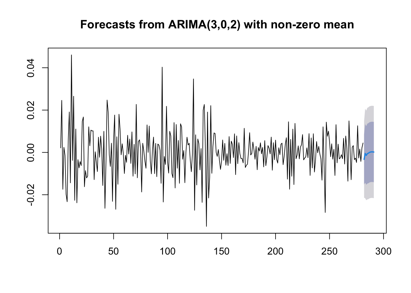 If you are interested in obtaining more forecasts, you can use use the
 h option:
plot(forecast(mod9, h=50))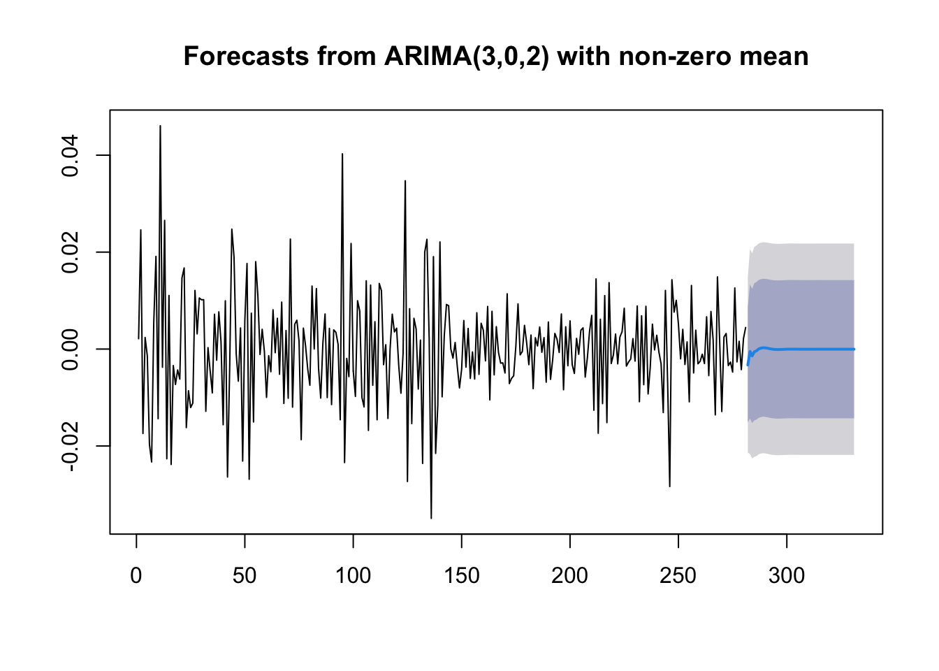 As expected for stationary models, the \(k\)-step forecast \(\hat y_{n+k}\) converges to the estimated mean \(\hat \mu\) as \(k\rightarrow +\infty\). Moreover, the \(k\)-step forecast error converges to a finite value as \(k\rightarrow +\infty\) and the forecast bounds converge to parallel horizontal lines.
We conclude by estimating for the (non-stationary) original data (logGNP) the same model that we have identified for the (stationary) second order differences (ARMA(3,2)); it will be an ARMA(3,2,1) model:
mod9original = Arima(GNPdf$logGNP, order=c(3,2,2),include.constant = TRUE)
summary(mod9original)
## Series: GNPdf$logGNP
## ARIMA(3,2,2)
##
## Coefficients:
## ar1 ar2 ar3 ma1 ma2
## 1.0211 -0.0723 -0.2566 -1.6265 0.6547
## s.e. 0.1679 0.1102 0.0614 0.1712 0.1643
##
## sigma^2 estimated as 8.515e-05: log likelihood=919.79
## AIC=-1827.59 AICc=-1827.28 BIC=-1805.76
##
## Training set error measures:
## ME RMSE MAE MPE MAPE
## Training set -0.0002598555 0.009113036 0.006455361 -0.002162477 0.08893417
## MASE ACF1
## Training set 0.389448 -0.005570206plot(forecast(mod9original,h = 50))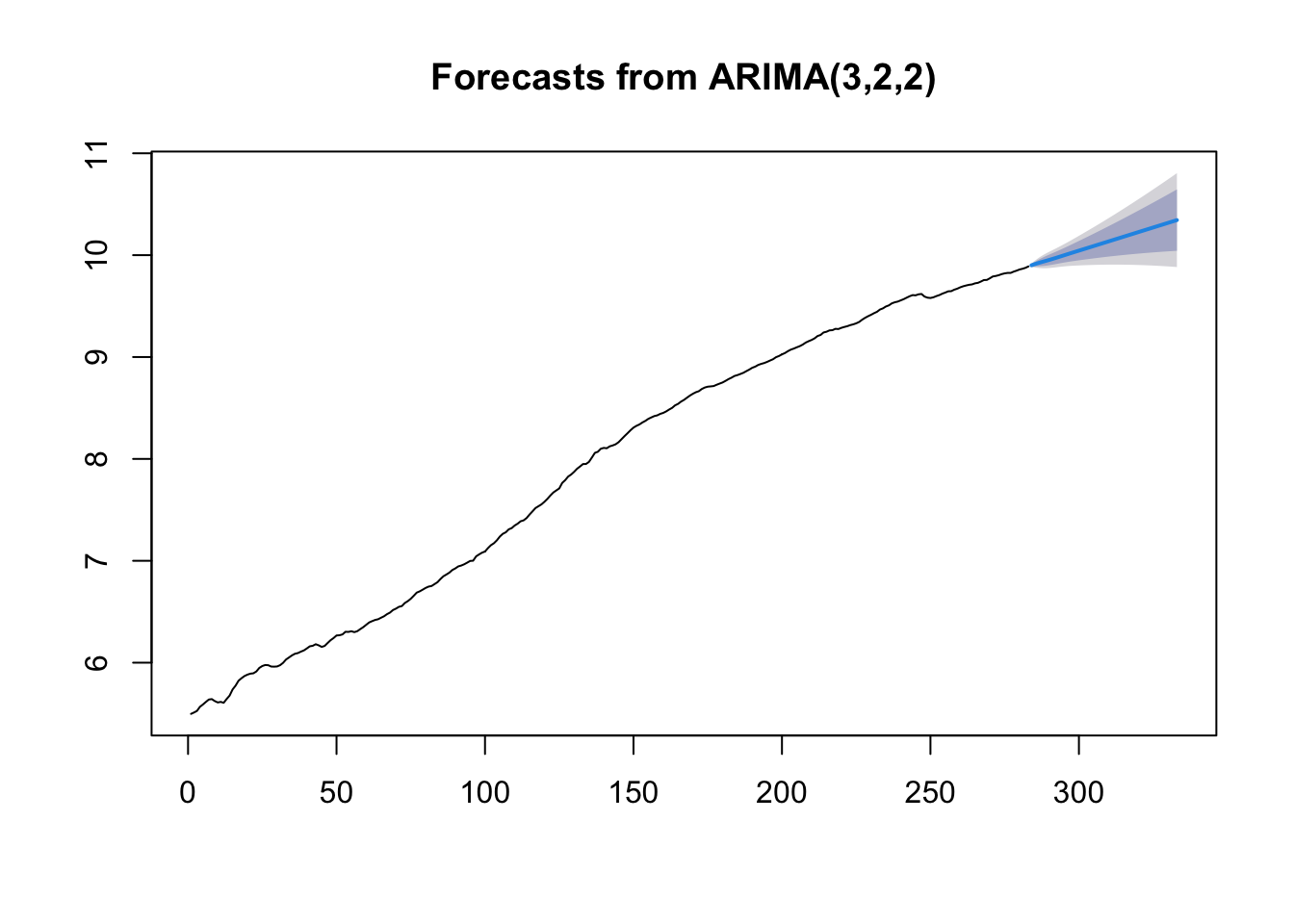 The parameter estimates do not change. We have however a different behavior of the prediction intervals. In fact, as expected for nonstationary models, the \(k\)-step forecast error converges to \(+\infty\) as \(k\rightarrow +\infty\) and the forecast bounds diverge away from each other.
12.5 Dynamic regression model
In order to illustrate how to implement a dynamic regression model, also known as ARIMAX, we use the data named usconsumption available in the fpp library. They refer to the percentage changes in quarterly personal consumption expenditure and personal disposable income for the US, 1970 to 2010.
library(fpp)## Loading required package: fma##
## Attaching package: 'fma'## The following objects are masked from 'package:faraway':
##
## airpass, eggs, ozone, wheat## The following objects are masked from 'package:MASS':
##
## cement, housing, petrol## Loading required package: expsmooth## Loading required package: lmtest## Loading required package: zoo##
## Attaching package: 'zoo'## The following object is masked from 'package:timeSeries':
##
## time<-## The following objects are masked from 'package:base':
##
## as.Date, as.Date.numerichead(usconsumption)## consumption income
## 1970 Q1 0.6122769 0.496540
## 1970 Q2 0.4549298 1.736460
## 1970 Q3 0.8746730 1.344881
## 1970 Q4 -0.2725144 -0.328146
## 1971 Q1 1.8921870 1.965432
## 1971 Q2 0.9133782 1.490757tail(usconsumption)## consumption income
## 2009 Q3 0.5740010 -1.3925562
## 2009 Q4 0.1093289 -0.1447134
## 2010 Q1 0.6710180 1.1871651
## 2010 Q2 0.7177182 1.3543547
## 2010 Q3 0.6531433 0.5611698
## 2010 Q4 0.8753521 0.3710579class(usconsumption)## [1] "mts" "ts"Note that the object usconsumption is of type Time-Series. For this reason in order to select a variable (i.e a column) it is not possible to use $ but we have to use square parentheses. Here below we represent graphically the two variables:
#consumption
ts.plot(usconsumption[,1])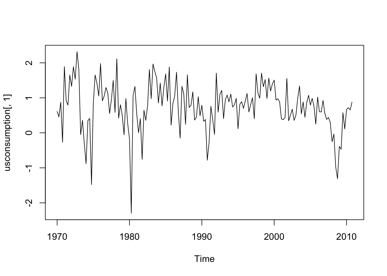
#income
ts.plot(usconsumption[,2])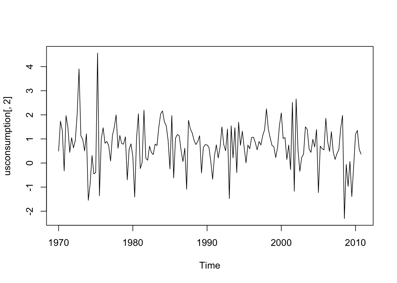
#both the variables together
ts.plot(usconsumption[,1],ylim=range(usconsumption))
lines(usconsumption[,2],col="red")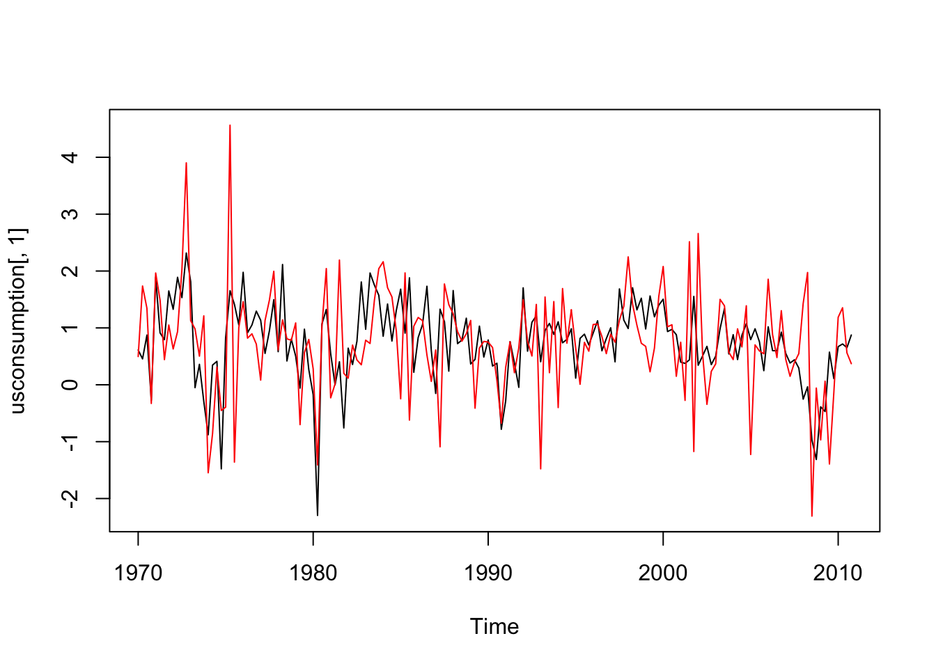 Both the time series appear to be stationary.
We start by implementing a standard simple regression model where consumption is the response variable and income the regressor:
modreg = lm(consumption ~ income, data=usconsumption)
summary(modreg)
##
## Call:
## lm(formula = consumption ~ income, data = usconsumption)
##
## Residuals:
## Min 1Q Median 3Q Max
## -2.3681 -0.3237 0.0266 0.3436 1.5581
##
## Coefficients:
## Estimate Std. Error t value Pr(>|t|)
## (Intercept) 0.52062 0.06231 8.356 2.79e-14 ***
## income 0.31866 0.05226 6.098 7.61e-09 ***
## ---
## Signif. codes: 0 '***' 0.001 '**' 0.01 '*' 0.05 '.' 0.1 ' ' 1
##
## Residual standard error: 0.6274 on 162 degrees of freedom
## Multiple R-squared: 0.1867, Adjusted R-squared: 0.1817
## F-statistic: 37.18 on 1 and 162 DF, p-value: 7.614e-09The slope \(\beta\) is positive and significantly different from zero. We can now proceed with the check of the uncorrelation hypothesis for the regression residuals:
acf(modreg$residuals) 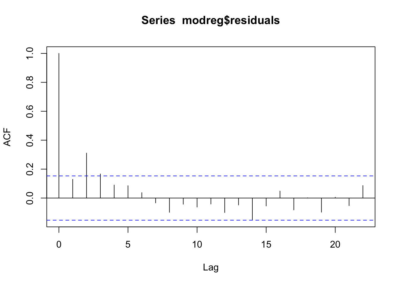
pacf(modreg$residuals) 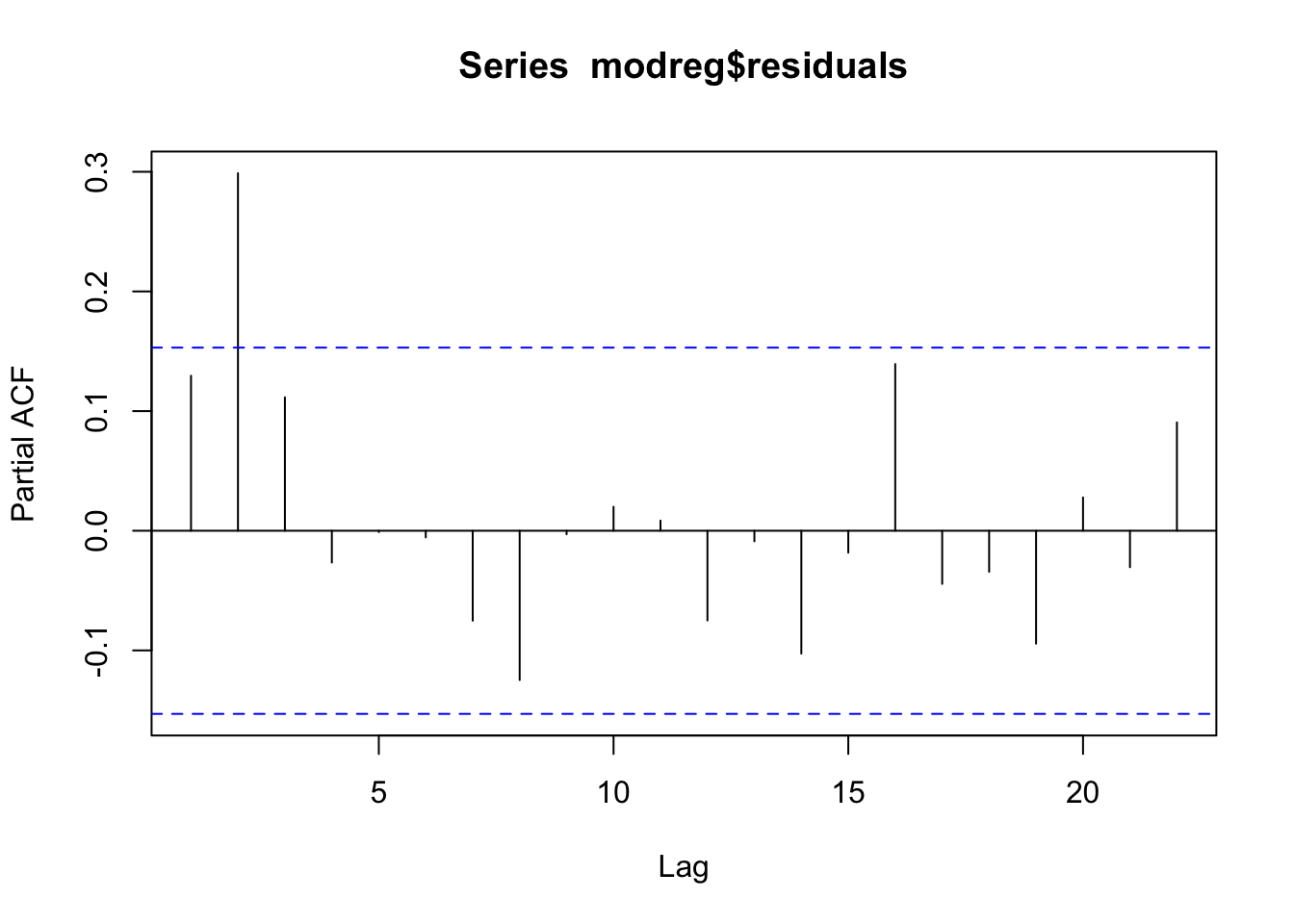 From the acf and pacf plots we observe that the residuals are correlated; thus the uncorrelation assumpation is not valid. The temporal pattern in the two plots is not clear: is it a cut-off at lag 3 for the acf? And a cut-off at lag 2 for the pacf? It is thus necessary to try different ARMA models. It results that the best one si the ARMA(1,2) model. Note that to include a regressor in an ARMA model we use the
 xreg argument in the function Arima:
modarimax = Arima(usconsumption[,1], order=c(1,0,2),
      xreg = usconsumption[,2], include.constant = TRUE)

summary(modarimax)
## Series: usconsumption[, 1]
## Regression with ARIMA(1,0,2) errors
##
## Coefficients:
## ar1 ma1 ma2 intercept xreg
## 0.6516 -0.5440 0.2187 0.5750 0.2420
## s.e. 0.1468 0.1576 0.0790 0.0951 0.0513
##
## sigma^2 estimated as 0.3502: log likelihood=-144.27
## AIC=300.54 AICc=301.08 BIC=319.14
##
## Training set error measures:
## ME RMSE MAE MPE MAPE MASE ACF1
## Training set 0.001835782 0.5827238 0.4375789 -Inf Inf 0.6298752 0.000656846modarimax$coef## ar1 ma1 ma2 intercept xreg
## 0.6516382 -0.5440223 0.2186652 0.5749932 0.2419798The estimated model is given by the following two equations:
\(Y_t=\) 0.57+ 0.24 \(x_t+u_t\)
\(u_t\) = 0.65 \(u_{t-1}+\epsilon_t\) -0.54 \(\epsilon_{t-1}\) + 0.22 \(\epsilon_{t-2}\)
where \(u_t\) are the correlated regression errors and \(\epsilon_t\) are the ARMA errors that should be as realizations from the white-noise process. We thus check if the ARMA errors are uncorrelated:
checkresiduals(modarimax, lag=14)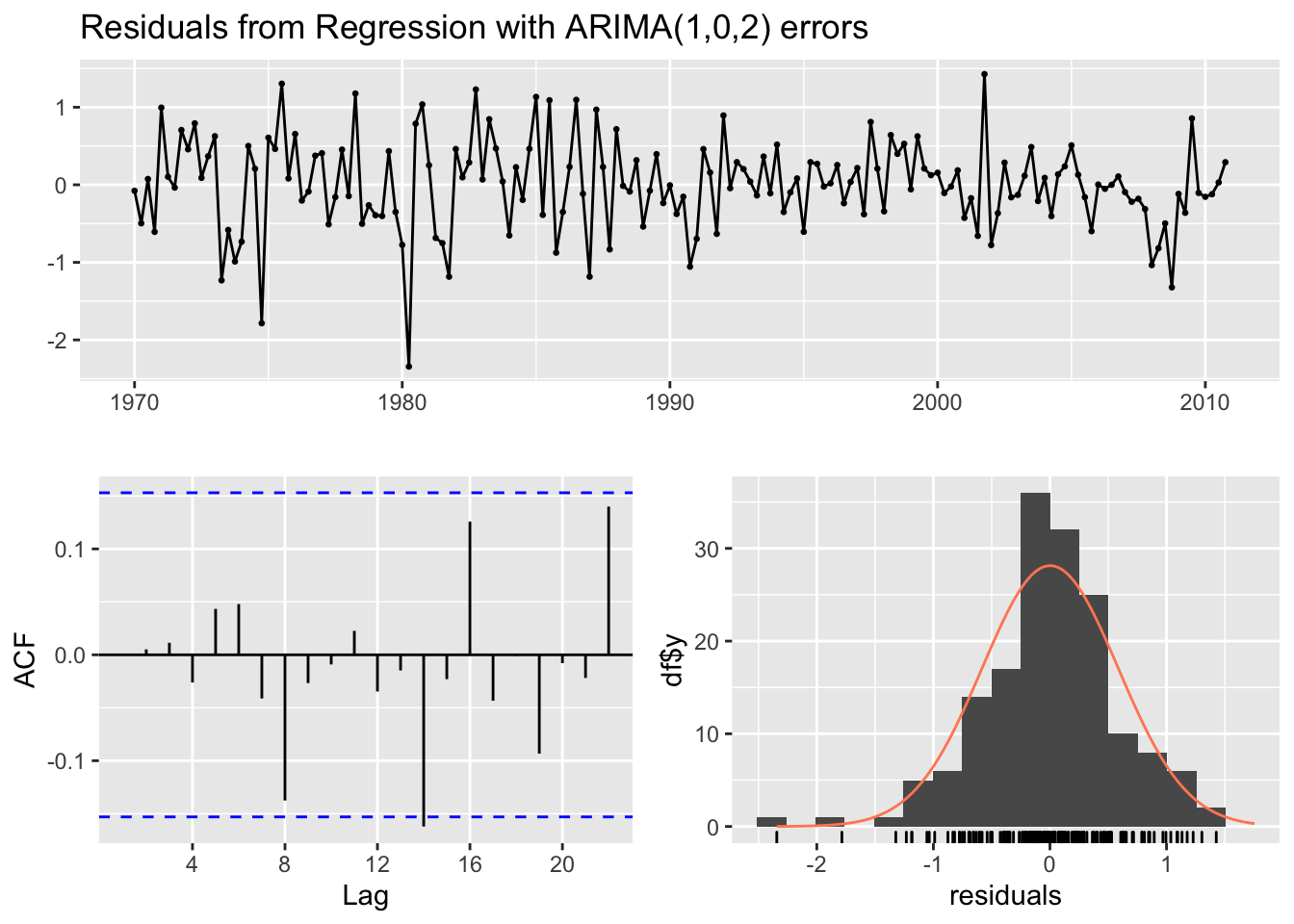
##
##  Ljung-Box test
##
## data:  Residuals from Regression with ARIMA(1,0,2) errors
## Q* = 9.7082, df = 9, p-value = 0.3746
##
## Model df: 5.   Total lags used: 14
We are interested in testing if the autocorrelation for lag \(h=14\) is a false positive or a significant correlation (we thus choose lag=14). Given the p-value we can conclude that the ARMA residuals are uncorrelated.