Chapter 5 Lab 3 - 23/10/2021

In this lecture we will learn how to compute jontly returns and how to study the their marginal distribution.

For this lecture we use the same set of data of Lab 2 included in the Adjcloseprices.csv file. We first proceed with the data import as described in Lab 2; the object prices will be created:

prices = read.csv("~/Dropbox/UniBg/Didattica/Economia/2021-2022/PSBF_2122/R_LABS/Lab03/prices.csv", sep=",", dec=".")
class(prices)

## [1] "data.frame"

head(prices)

##       Date   A2Aadj   ISPajd  JUVEadj
## 1 10/01/17 0.982659 1.597666 0.288256
## 2 11/01/17 0.999368 1.595077 0.289546
## 3 12/01/17 1.012895 1.573067 0.288164
## 4 13/01/17 1.030400 1.596372 0.289546
## 5 16/01/17 1.021647 1.566594 0.284573
## 6 17/01/17 1.022443 1.566594 0.288256

str(prices)

## 'data.frame':    1213 obs. of  4 variables:
##  $ Date   : chr  "10/01/17" "11/01/17" "12/01/17" "13/01/17" ...
##  $ A2Aadj : num  0.983 0.999 1.013 1.03 1.022 ...
##  $ ISPajd : num  1.6 1.6 1.57 1.6 1.57 ...
##  $ JUVEadj: num  0.288 0.29 0.288 0.29 0.285 ...

Note that in the previous code the entire path of the file is used; this will be obviously different in your case. If you are not sure how to specify the path, use the RStudio feature to import data, as described in Section 4.1.

5.1 Compute returns jointly

We start by computing log returns using the definition provided in Section 4.5. One possibility is to perform the computation separately for each asset, starting for example with A2A:

logretA2A = diff(log(prices$A2Aadj))

The output is a vector. This code should be repeated for all the remaining assets giving rise to a number of code lines equal to the number of considered assets. This could result in a long list of code lines when the number of assets is large. An alternative is to compute the log returns jointly for all the available assets by using the apply function introduced in Section 4.3. In particular, we first compute log prices by applying the log function column by column (the second argument is set equal to 2); note that we exclude the first column of prices as it contains dates:

logprices = apply(prices[,-1],2,log)
head(logprices)

##             A2Aadj    ISPajd   JUVEadj
## [1,] -0.0174931163 0.4685438 -1.243906
## [2,] -0.0006321998 0.4669220 -1.239441
## [3,]  0.0128125674 0.4530272 -1.244226
## [4,]  0.0299470764 0.4677336 -1.239441
## [5,]  0.0214160309 0.4489038 -1.256765
## [6,]  0.0221948617 0.4489038 -1.243906

We then compute the differences of the log prices by means of the diff function:

logret = apply(logprices, 2, diff)
head(logret)

##             A2Aadj       ISPajd      JUVEadj
## [1,]  0.0168609165 -0.001621803  0.004465205
## [2,]  0.0134447672 -0.013894794 -0.004784417
## [3,]  0.0171345090  0.014706338  0.004784417
## [4,] -0.0085310454 -0.018829719 -0.017324368
## [5,]  0.0007788307  0.000000000  0.012859163
## [6,]  0.0092950844 -0.002482982  0.000000000

We check which kind of object logret is

class(logret)

## [1] "matrix" "array"

and we realize that it is not a data frame but rather a matrix. As we prefer working with data frame we transform the matrix into a data frame as follows:

logret = data.frame(logret)
class(logret)

## [1] "data.frame"

5.2 Boxplot

We aim to use boxplots to study and compare the available log returns distributions. It is possible to obtain a plot containing the boxplots of all the assets by using the following code:

boxplot(logret,
        horizontal = TRUE,
        col = rainbow(ncol(logret)))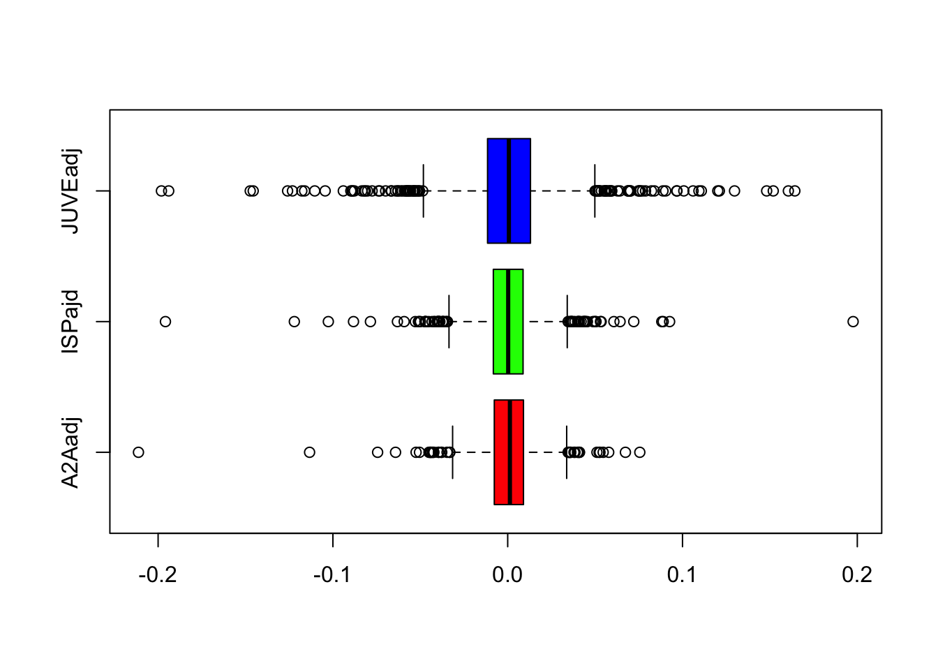

We note that JUVE is characterized by higher variability and a larger number of extreme events. Moreover, for all the assets the median log return value is close to zero, the whiskers are symmetric and the median is placed in the middle of the box.

If you want to define the whiskers by using the minimum and maximum value use the range option of the boxplot function (see ?boxplot); in this case outliers are not shown:

boxplot(logret, range = 0,
        horizontal = TRUE,
        col = rainbow(ncol(logret)))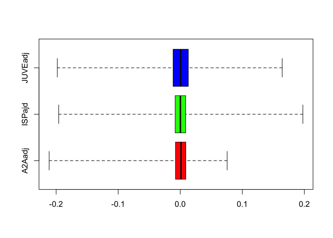

5.3 Histogram and Kernel Density Estimator

The A2A log returns can be represented graphically by using the histogram:

hist(logret$A2Aadj)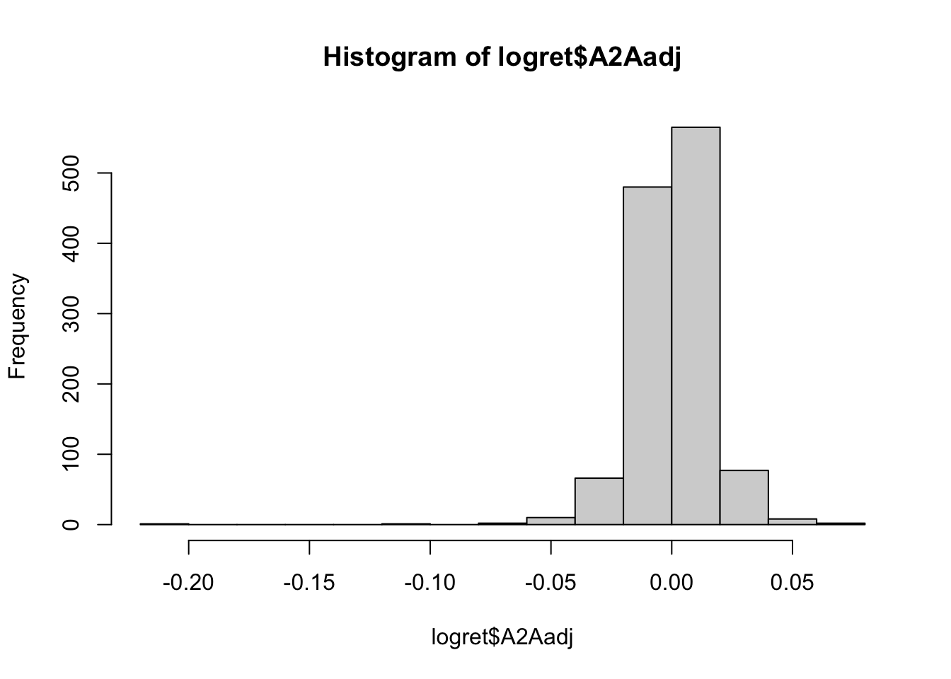

The plot represents the values of the log returns on the x-axis (with classes of values set automatically by R) and the corresponding frequencies (i.e. number of days) on the y-axis. From the histogram a very long tail on the left is clearly visible.

By using the breaks arguments it is possible to specify a different number of classes of values. If the breaks parameter is a single integer value the hist function will use a number of bins as close as possible of the specified value of breaks.

hist(logret$A2Aadj, breaks=3)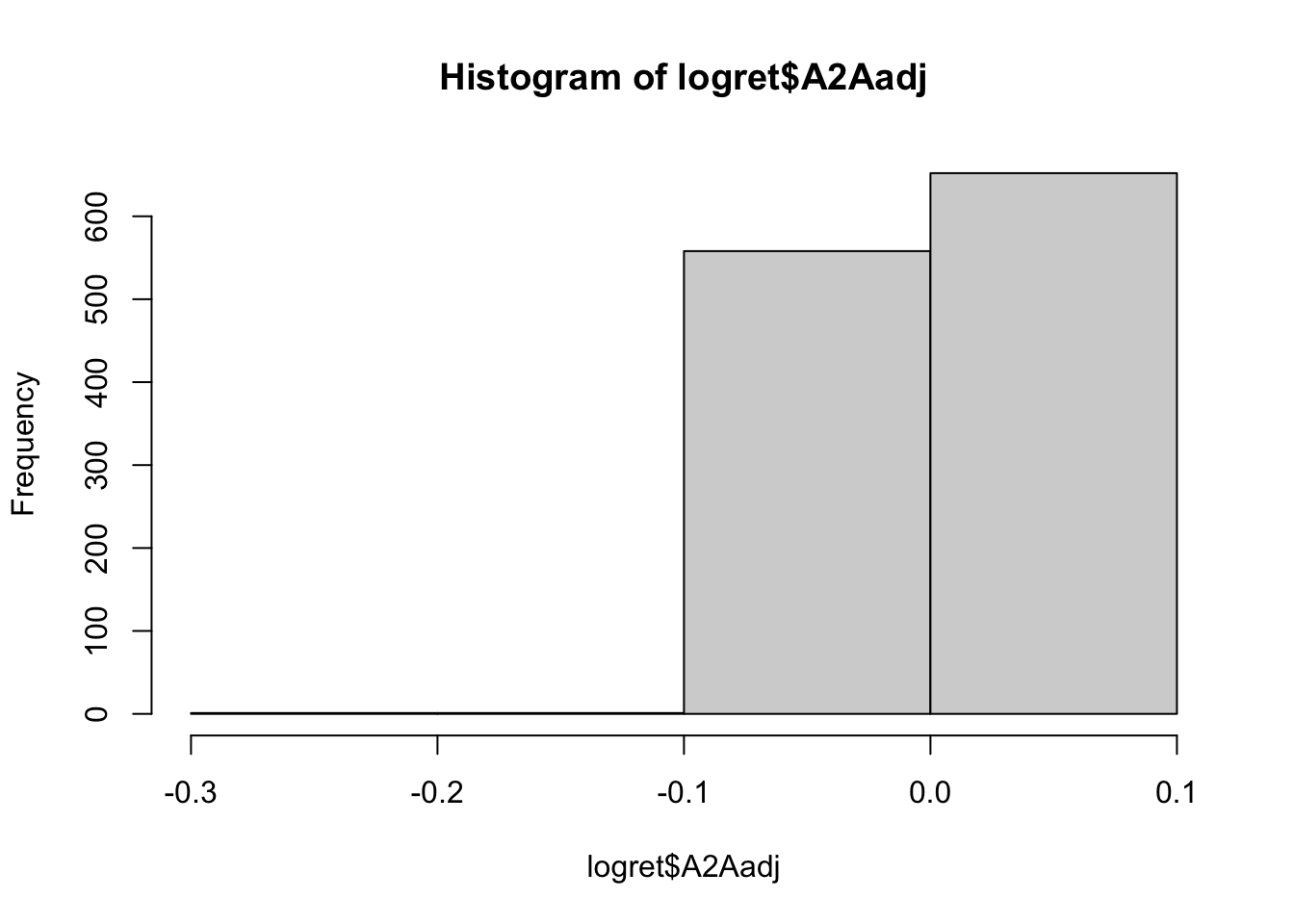

hist(logret$A2Aadj, breaks=20)

Note that the classes are equally sized. It is also possible to set the limits of the classes by providing to breaks a vector of values:

hist(logret$A2Aadj,
     breaks = c(-0.25,0, 0.01, 0.15))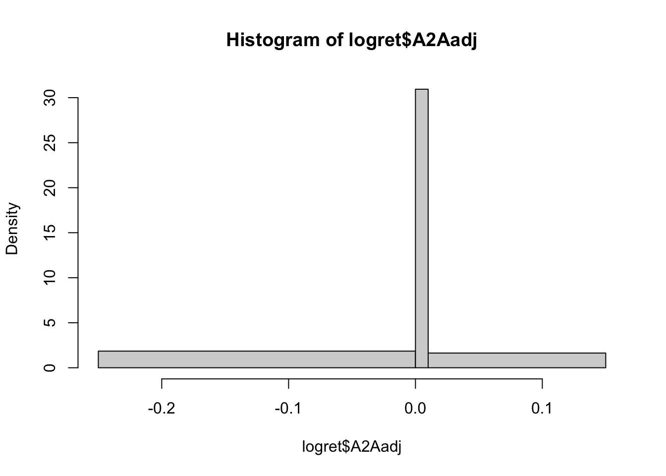

In this case the used class are \([-0.25,0]\),\((0,0.01]\) and \((0.01,0.15]\).

The plot of the Kernel Density Estimator (KDE) can be obtained by using the plot and density functions:

plot(density(logret$A2Aadj))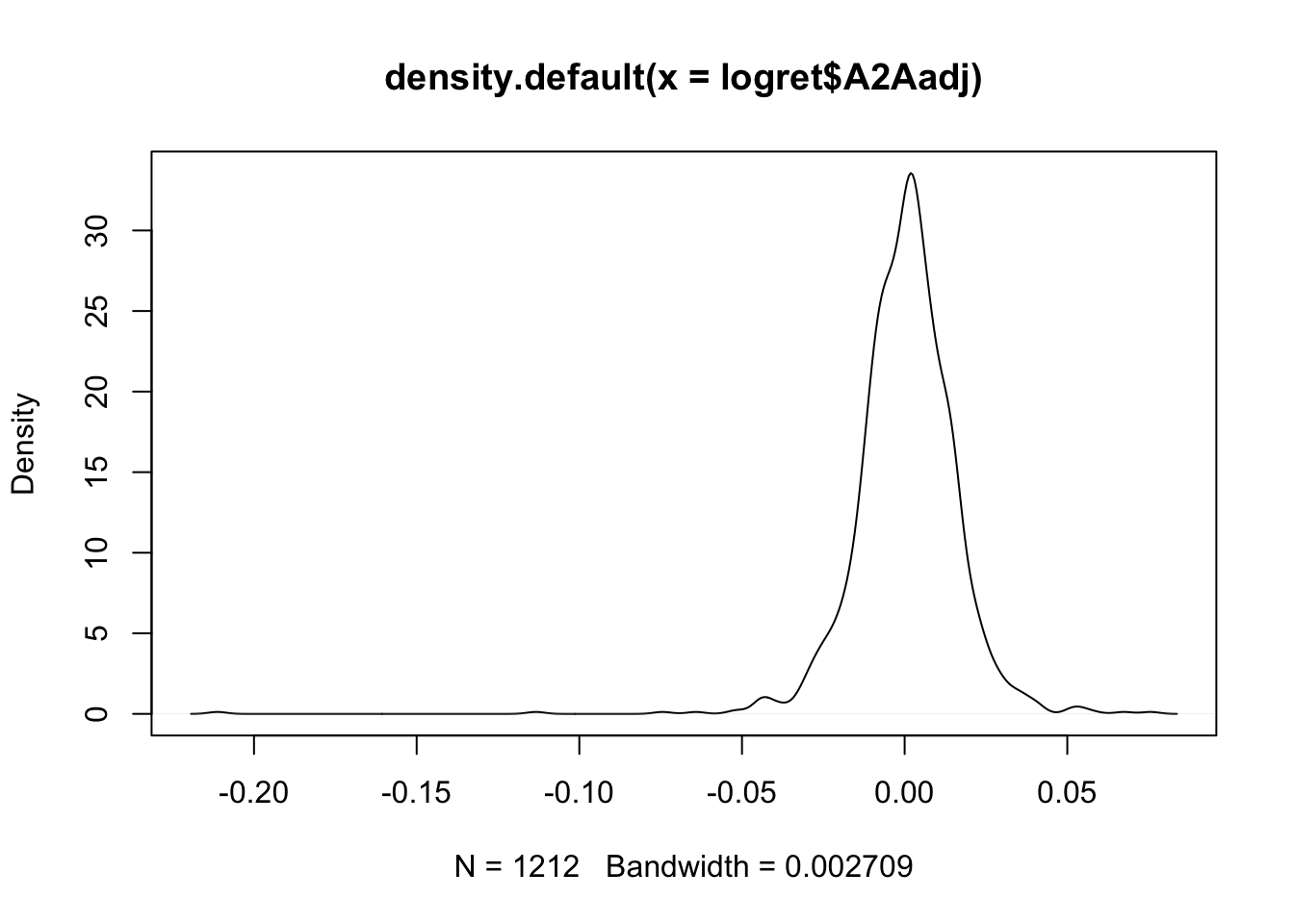

Note that by default R sets the best value for the bandwidth parameter (see the bottom of the plot). In order to study the effect of the bandwidth on the final KDE, we double its value by using the adjust argument:

plot(density(logret$A2Aadj,adjust=2))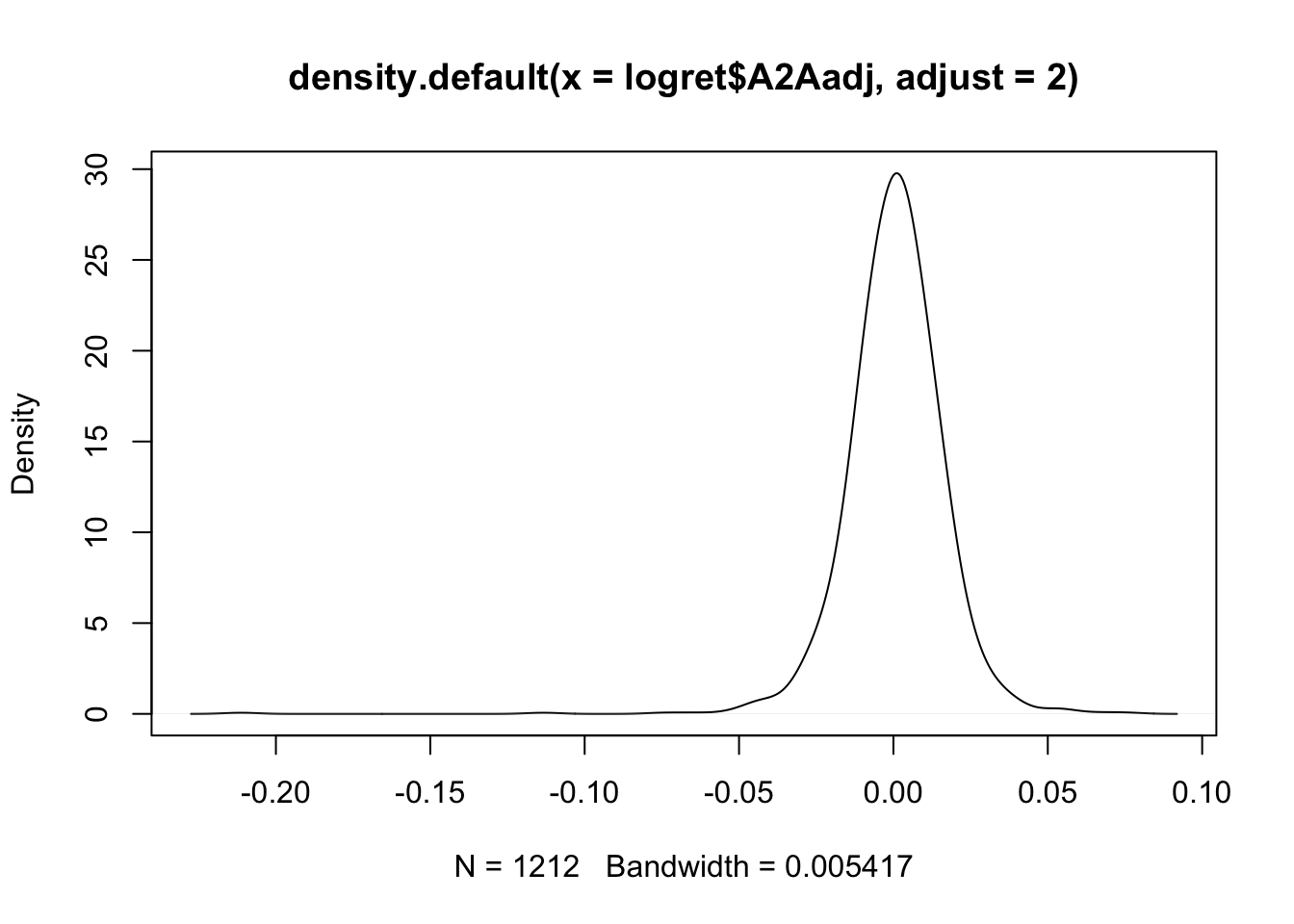

The multiplicative constant specified with adjust is applied to the original value set automatically by R. When the bandwidth is doubled the KDE line is smoother. If instead the bandwidth is halved:

plot(density(logret$A2Aadj,adjust=0.5))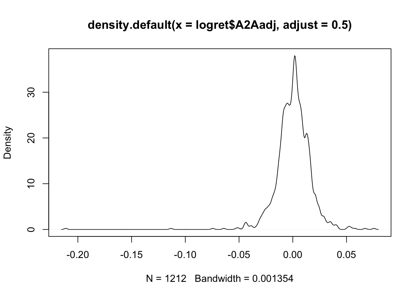

the final KDE is characterized by more bumps, is less smooth and shows more fine details of the distribution.

It is also possible to plot together the histogram and the KDE line:

hist(logret$A2Aadj, freq = F, ylim = c(0,35))
lines(density(logret$A2Aadj),
      col = "red", 
      lwd = 1.5)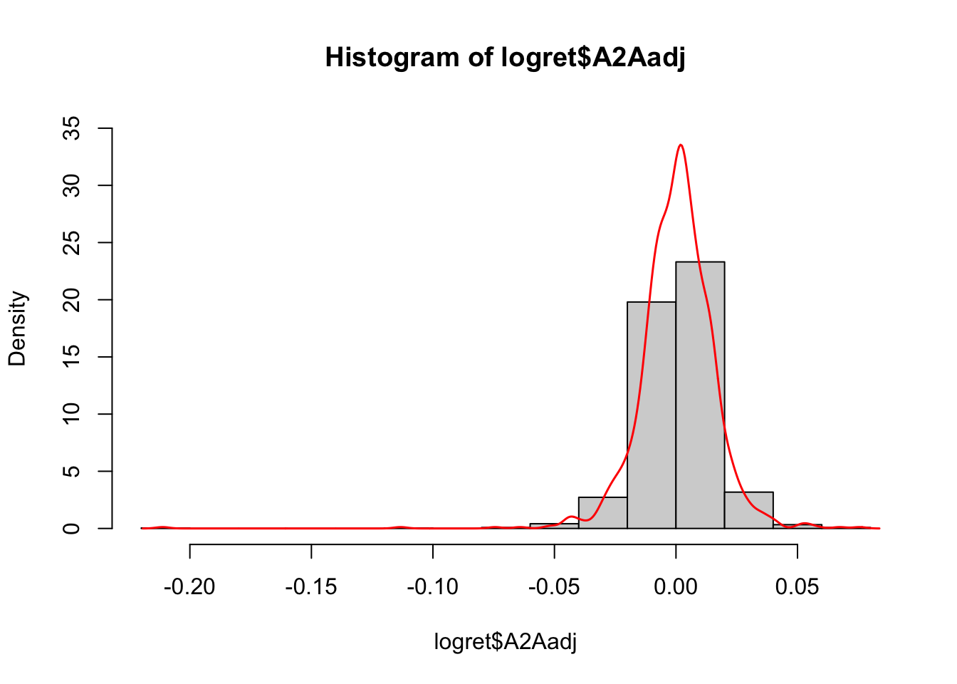

Note that the argument freq=F is used to represent densities instead of frequencies in the y-axis. In this way th histogram and the KDE are comparable and can be plotted together. Finally, note that in the density histogram the area of each single bar is represented by the absolute frequency of the class of values.

5.4 Sample skewness and kurtosis index

In order to evaluate the asymmetry of the distribution it is possible to compute the skewness index given by this formula: \[ sk = \frac{\frac{\sum_{i=1}^n (x_i-\bar x)^3}{n}}{\sigma^3} \] which is implemented in R as follows

mean((logret$A2Aadj - mean(logret$A2Aadj))^3) / 
  sd(logret$A2Aadj)^3

## [1] -2.206542

where the function sd computes the standard deviation. The skewness index is negative and suggests a negative skewness (long left tail).

The sample kurtosis instead is given by \[ sk = \frac{\frac{\sum_{i=1}^n (x_i-\bar x)^4}{n}}{\sigma^4} \] and can be computed as follows:

mean((logret$A2Aadj - mean(logret$A2Aadj))^4) / 
  sd(logret$A2Aadj)^4

## [1] 31.29707

The kurtosis value is extremely bigger than three, meaning that the distribution is characterized by excess of kurtosis (with respect to the normal distribution).

5.5 Remove rows with missing data

We now use a new set of data available in the posteit.csv file. We first proceed with the data import; the object poste will be created:

poste = read.csv("~/Dropbox/UniBg/Didattica/Economia/2021-2022/PSBF_2122/R_LABS/Lab03/posteit.csv", sep=";", dec=".")
head(poste)

##         Date   PSTadj
## 1 2017-01-10 4.706218
## 2 2017-01-11 4.717724
## 3 2017-01-12 4.679369
## 4 2017-01-13 4.729231
## 5 2017-01-16 4.652520
## 6 2017-01-17 4.641014

The function summary can be applied to the data frame in order to get the main summary statistics for all the variables included in the data frame:

summary(poste)

##      Date               PSTadj      
##  Length:1213        Min.   : 4.461  
##  Class :character   1st Qu.: 5.518  
##  Mode  :character   Median : 7.213  
##                     Mean   : 7.414  
##                     3rd Qu.: 8.966  
##                     Max.   :12.555  
##                     NA's   :3

It is worth to note that the PSTadj time series have 3 missing values (NA), i.e. three days for which prices are not available.

In order to find the missing values, we will use the is.na function. It returns, for each element in a vector, TRUE or FALSE according if the value is missing or not. See for example what happens with the first 20 values:

head(is.na(poste$PSTadj), n=20)

##  [1] FALSE FALSE FALSE FALSE FALSE FALSE FALSE FALSE FALSE FALSE FALSE FALSE
## [13] FALSE  TRUE FALSE FALSE FALSE FALSE FALSE FALSE

The following command

sum(is.na(poste$PSTadj))

## [1] 3

returns the number of missing values in the vector.

We want to create a new data frame containing only the non missing values. Remembering what was done in Lab. 1, we need to set a proper condition equal to TRUE if the value is not missing. We thus need to use the complement of the is.na function obtained using the ! operator and the squared parenthesis with the 2 indexes for the selection (all the columns and only the rows satisfying the condition):

poste2 = poste[!is.na(poste$PSTadj),]

We want now instead to substitie in poste the missing value with the median computed using the non missing value. For computing the median we have to specify the option na.rm = TRUE, otherwise the function will return NA:

median(poste$PSTadj, na.rm = TRUE)

## [1] 7.212518

Finally, the substitution:

poste$PSTadj[is.na(poste$PSTadj)] = median(poste$PSTadj, na.rm = TRUE)

Note that now there are no more missing values:

summary(poste)

##      Date               PSTadj      
##  Length:1213        Min.   : 4.461  
##  Class :character   1st Qu.: 5.520  
##  Mode  :character   Median : 7.213  
##                     Mean   : 7.413  
##                     3rd Qu.: 8.965  
##                     Max.   :12.555

5.6 Exercises Lab 3

5.6.1 Exercise 1

The file AdjclosepricesLab3.csv contains the daily adjusted close prices observed from 01-09-2016 to 27-08-2020 for the following indexes: NASDAQ Composite (IXIC), Dow Jones Industrial Average (DJI), Gold (Gold) and CBOE Volatility Index (VIX). Data source: Yahoo Finance.

Import the data in R and check the structure of the data. Are there any missing values?
Compute for the 4 assets the gross returns by using less code as possible. Create a new data frame containing all the net returns.
Provide altogether the boxplots of the 4 distributions (one single plot is required). Comment the plot.
Provide now the same plot but removing VIX. What do you observe? Hint: for not selecting one column of the data frame it is possible to use the - symbol; e.g. mydata[,-1] for omitting the first column of mydata.
Represent in the same plot the KDE and the histogram for IXIC. Comment the plot.
Represent in the same plot the 4 KDEs for the gross return time series. Comment the plot.
Compute for the gross return distributions the sample skeweness. Comment the values.
Compute for the gross return distributions the sample kurtosis Comment the values.