8 Unsupervised Learning
This chapter will cover the concepts seen in Unsupervised Learning. We will discuss more in detail how to implement several dimensionality reduction and clustering methods. Make sure that you go over the video and slides before going over this chapter. Note that some of the materials are already covered in data mining, however we repeat how to implement these methods in R for didactical reasons.
8.1 Dimensionality reduction
In a lot of cases, you are confronted with a large number of variables. If you want to visualize that relationship into one graph this often impossible. However, such a plot should reduce the number of variables to a minimum but maintain the variance as much as possible. Another problem , especially in parametric methods, is often the presence of multicollinearity. to solve both of these issues, you can make use of principal components analysis (PCA), one of the most well-known feature extraction methods.
We will show you how to implement PCA in R, making use of the football data set also used in Session 2. To perform PCA in R, you can make use of the stats package and the function princomp which is by default in R. However, a better package is the psych package, since this one has more option.
# load the packages
if (!require("pacman")) install.packages("pacman")
require("pacman", character.only = TRUE, quietly = TRUE)
p_load(tidyverse, psych)

# Set working directory
setwd("C:\\Users\\matbogae\\OneDrive - UGent\\PPA22\\PredictiveAnalytics\\Book_2022\\data codeBook_2022")

# Read in the data
football <- read_csv("football_players.csv")
## Rows: 10390 Columns: 32## -- Column specification --------------------------
## Delimiter: ","
## chr (1): player_name
## dbl (31): overall_rating, potential, crossing,...##
## i Use `spec()` to retrieve the full column specification for this data.
## i Specify the column types or set `show_col_types = FALSE` to quiet this message.football %>%
glimpse()## Rows: 10,390
## Columns: 32
## $ player_name <chr> "Aaron Appindangoye",~
## $ overall_rating <dbl> 63.60000, 66.96970, 6~
## $ potential <dbl> 67.60000, 74.48485, 7~
## $ crossing <dbl> 48.60000, 70.78788, 6~
## $ finishing <dbl> 43.60000, 49.45455, 5~
## $ heading_accuracy <dbl> 70.60000, 52.93939, 5~
## $ short_passing <dbl> 60.60000, 62.27273, 6~
## $ volleys <dbl> 43.60000, 29.15152, 5~
## $ dribbling <dbl> 50.60000, 61.09091, 6~
## $ curve <dbl> 44.60000, 61.87879, 6~
## $ free_kick_accuracy <dbl> 38.60000, 62.12121, 5~
## $ long_passing <dbl> 63.60000, 63.24242, 6~
## $ ball_control <dbl> 48.60000, 61.78788, 6~
## $ acceleration <dbl> 60.00000, 76.00000, 7~
## $ sprint_speed <dbl> 64.00000, 74.93939, 7~
## $ agility <dbl> 59.00000, 75.24242, 7~
## $ reactions <dbl> 46.60000, 67.84848, 5~
## $ balance <dbl> 65.00000, 84.72727, 8~
## $ shot_power <dbl> 54.60000, 65.90909, 6~
## $ jumping <dbl> 58.00000, 75.30303, 6~
## $ stamina <dbl> 54.00000, 72.87879, 7~
## $ strength <dbl> 76.00000, 51.75758, 7~
## $ long_shots <dbl> 34.60000, 54.12121, 5~
## $ aggression <dbl> 65.80000, 65.06061, 5~
## $ interceptions <dbl> 52.20000, 57.87879, 4~
## $ positioning <dbl> 44.60000, 51.48485, 6~
## $ vision <dbl> 53.60000, 57.45455, 6~
## $ penalties <dbl> 47.60000, 53.12121, 6~
## $ marking <dbl> 63.80000, 69.39394, 2~
## $ standing_tackle <dbl> 66.00000, 68.78788, 2~
## $ sliding_tackle <dbl> 67.80000, 71.51515, 2~
## $ gk_reflexes <dbl> 7.60000, 12.90909, 13~# Since PCA can only be applied to numeric data, select the
# numerics
nums <- football %>%
select_if(is.numeric)
# Before applying PCA, you should always check the mean and
# the variance If the differences in mean and variances are
# large, you should scale the data
nums %>%
summarize_all(mean)## # A tibble: 1 x 31
## overall_rating potential crossing finishing
## <dbl> <dbl> <dbl> <dbl>
## 1 66.9 72.1 53.0 47.9
## # ... with 27 more variables:
## # heading_accuracy <dbl>, short_passing <dbl>,
## # volleys <dbl>, dribbling <dbl>, curve <dbl>,
## # free_kick_accuracy <dbl>, long_passing <dbl>,
## # ball_control <dbl>, acceleration <dbl>,
## # sprint_speed <dbl>, agility <dbl>,
## # reactions <dbl>, balance <dbl>, ...nums %>%
summarize_all(var)## # A tibble: 1 x 31
## overall_rating potential crossing finishing
## <dbl> <dbl> <dbl> <dbl>
## 1 37.9 32.7 259. 327.
## # ... with 27 more variables:
## # heading_accuracy <dbl>, short_passing <dbl>,
## # volleys <dbl>, dribbling <dbl>, curve <dbl>,
## # free_kick_accuracy <dbl>, long_passing <dbl>,
## # ball_control <dbl>, acceleration <dbl>,
## # sprint_speed <dbl>, agility <dbl>,
## # reactions <dbl>, balance <dbl>, ...# We notice a huge difference in variance for several
# variable the difference in mean is acceptable, however
# gkreflexes has a much lower mean so it is best to scale
# your data
football_sc <- nums %>%
scale()
describe(football_sc)## [322090 obs.]
## matrix: -0.529293869002172 0.0178629575440086 0.0227834326028726 0.361654410570158 1.03600765672507 1.68863759975536 -1.02106020488565 2.09619592279377 -3.06235442930767 0.0313295208630174 -0.788725518174457 0.414587954646997 0.363458539411657 -0.232478575249716 0.448695959774505 1.40440273422724 0.679401659053123 1.72806392850139 -2.66633034347231 -0.470447320605076 -0.272007786831898 1.10726772574523 0.941136217417357 0.263679149355763 -0.490823197294831 1.30003727066063 -0.335947354824312 1.55798910093393 -2.54719074789534 0.678766110903274 -0.238247687132312 0.0857380576376712 0.55437964497217 -1.19778094743271 -0.501662183967035 1.37847620878451 -0.903898966648627 0.999221515030812 -1.82094823534094 -0.102521066693366 0.935947814191637 -0.202261987107591 0.168508007824898 0.849642090545631 1.09320356779598 0.608451010996183 -0.612671492380447 -1.6509390783288 -2.58297191810236 0.0492641646623795 0.00791916448861004 0.132978661754365 0.34550661174821 0.314125806895916 0.318936696819091 1.32819301968068 0.23007454472467 1.17941086818164 -2.80320083926766 0.632000397125428 -0.206093397482575 -1.0434602263044 0.412245482260651 0.0363111048862791 -0.873738895898907 1.76825179748702 -0.787302648336076 1.23030737435064 -1.92157141424676 0.698619937816604 -0.38695617156069 0.238103190669443 0.71162669765154 -0.0911233138885098 -0.38695617156069 1.29411207531525 -0.209915342050594 1.67408978707402 -2.50804149434509 0.753236943998757 -0.340369386633345 0.664065094670231 0.566028191664115 -0.736671658914407 -0.289214042303188 1.59259644415855 0.297411529690698 0.675582906357198 -2.11918022356837 1.18817188294481 -0.536034900247331 0.913370920103573 0.512473882801592 -0.425652538386924 -1.2902786505129 1.30301621922737 -0.476174285146887 0.434262332528953 -1.805432061642 1.05184667925914 0.650167367699465 0.622598429046503 0.408193319444292 0.436299853182366 0.128974246114541 0.792373248999753 0.647964522722354 -0.0870231763720679 -2.8655732157728 0.218409752185327 -0.874509418752489 0.0363907727010471 0.507973539380804 0.132125567439012 -0.0760484696814999 1.15873664789374 0.090511352616059 1.49090723367234 -2.71179845381203 0.7126698307667 -0.563974981127427 0.815126891143998 0.775345106366935 -1.40717585411947 -1.32937652023807 0.923667316276474 0.32259050818992 2.31688926647802 -4.44269899689081 0.656348715060116 -0.261186510746804 0.715859578351005 0.944558732170304 -1.25917854755742 -1.14718597813478 0.790739380193226 0.00675687656810907 2.1983963779388 -3.65513608340236 0.716571814893577 -0.447829292967689 0.892948676463125 1.08883156579731 -0.131993859545638 -1.12802396731028 1.15421138194923 -0.365281395596016 2.26990148203817 -2.75917041937454 0.364615802216676 -2.1879498336109 0.464969755389464 -1.72023437094443 -0.737493239451223 0.658679799537815 1.65842204561766 -0.443586562170143 1.6891904595812 -2.38771331663888 0.516742587912666 0.0450617448661233 1.80455605200356 1.4481040858465 -1.82019258874722 -0.0298586578894064 0.583510847562385 1.38292607978629 2.02784529764524 -3.61176743724901 0.857168867466784 -0.328325961855968 0.417024238579914 0.212619827317662 0.348512039951843 -0.823947895779249 1.11137959679233 -0.462023368043478 0.222759392250629 -2.21327108289398 0.405671807028177 -0.841760377684083 0.972775425949681 0.134319571650367 0.498727429127371 1.23882260192204 0.323440663761999 0.521524840807835 -0.260952473947886 -2.93912225228703 -0.0524899880308662 -1.01473710876829 0.6582878610437 0.484974124820427 -0.887587678094464 0.0912317573109561 0.829857213218101 0.225933093564197 1.32685747640318 -4.20503191476609 0.986193405519819 0.852472778518433 -1.35353172593797 0.313486485650767 1.09777088809005 0.652277869739013 -0.0743555028677695 -0.694487880231625 -1.4714681205993 -2.05945316736403 -0.0766614871085391 -0.9463487875562 0.188674751220707 0.416435725704812 -1.13796817931251 -1.54638544754668 1.37033022054656 -0.773580756994157 0.326984822307308 -2.26038255846557 0.582508389775714 0.427689254301564 0.377913527721286 -0.0223165814937412 0.663600654084585 0.688889419520381 -0.336762546539305 1.01817858215265 -0.470251044051779 -2.58823017915281 0.884045484363742 0.0857187277449564 0.411416581003319 -0.197077704812883 0.622845886700712 1.49890676638657 0.411995908383714 0.188954866931438 -0.417667745809642 -1.81841450613904 0.71117276398586 -0.545799658456469 -0.131012642846777 0.49090105522592 -1.06915711190123 -0.818113176274875 1.31469699146967 -0.5991607144133 1.30422682747116 -2.38933807554567 0.546878942384502 -0.164322328623037 0.111393339042496 0.9647513380218 -0.151260327140111 -0.67361598644295 1.72142062620538 0.293469723349918 1.61402371942575 -2.92538064208492 0.63606081487573 -0.421504466525904 -0.0202857437808091 0.518715343686425 -0.847405618212843 -0.0320008019860981 1.61267788324735 -0.859592276855854 0.731131234221917 -0.901117187787605 0.0741718387014968 0.887512168933577 1.16804242843979 -1.20678567681835 1.2289611950479 1.57956785787794 -0.722083805406695 0.274261993223046 -1.14699268251156 -1.55975722385519 0.82627764573179 0.820643741927127 0.958248694114398 -1.39478448285715 1.05026712858745 1.31620105452155 -0.881303498833549 0.383470244760734 -1.14609459644177 -1.69662945949871 0.750503002568514 1.00938079076002 1.19077562528086 -1.25876028008667 1.02126878473813 1.34139547971986 -0.722303665383463 0.461138048065832 -1.28129521372648 -1.71509268629279 0.71334292568128 -0.544579889436886 -0.225185651767604 -0.189636635588659 -0.389733606254754 -0.284689235771744 -0.108309399145089 -0.125179628231231 -0.212775048486198 2.18667836898845 -0.14689146228847 ...
## min: -4.72187984569954 - max: 4.4700190235591 - NAs: 0 (0%) - 322059 unique values [322090 obs.]
## array: -0.529293869002172 0.0178629575440086 0.0227834326028726 0.361654410570158 1.03600765672507 1.68863759975536 -1.02106020488565 2.09619592279377 -3.06235442930767 0.0313295208630174 -0.788725518174457 0.414587954646997 0.363458539411657 -0.232478575249716 0.448695959774505 1.40440273422724 0.679401659053123 1.72806392850139 -2.66633034347231 -0.470447320605076 -0.272007786831898 1.10726772574523 0.941136217417357 0.263679149355763 -0.490823197294831 1.30003727066063 -0.335947354824312 1.55798910093393 -2.54719074789534 0.678766110903274 -0.238247687132312 0.0857380576376712 0.55437964497217 -1.19778094743271 -0.501662183967035 1.37847620878451 -0.903898966648627 0.999221515030812 -1.82094823534094 -0.102521066693366 0.935947814191637 -0.202261987107591 0.168508007824898 0.849642090545631 1.09320356779598 0.608451010996183 -0.612671492380447 -1.6509390783288 -2.58297191810236 0.0492641646623795 0.00791916448861004 0.132978661754365 0.34550661174821 0.314125806895916 0.318936696819091 1.32819301968068 0.23007454472467 1.17941086818164 -2.80320083926766 0.632000397125428 -0.206093397482575 -1.0434602263044 0.412245482260651 0.0363111048862791 -0.873738895898907 1.76825179748702 -0.787302648336076 1.23030737435064 -1.92157141424676 0.698619937816604 -0.38695617156069 0.238103190669443 0.71162669765154 -0.0911233138885098 -0.38695617156069 1.29411207531525 -0.209915342050594 1.67408978707402 -2.50804149434509 0.753236943998757 -0.340369386633345 0.664065094670231 0.566028191664115 -0.736671658914407 -0.289214042303188 1.59259644415855 0.297411529690698 0.675582906357198 -2.11918022356837 1.18817188294481 -0.536034900247331 0.913370920103573 0.512473882801592 -0.425652538386924 -1.2902786505129 1.30301621922737 -0.476174285146887 0.434262332528953 -1.805432061642 1.05184667925914 0.650167367699465 0.622598429046503 0.408193319444292 0.436299853182366 0.128974246114541 0.792373248999753 0.647964522722354 -0.0870231763720679 -2.8655732157728 0.218409752185327 -0.874509418752489 0.0363907727010471 0.507973539380804 0.132125567439012 -0.0760484696814999 1.15873664789374 0.090511352616059 1.49090723367234 -2.71179845381203 0.7126698307667 -0.563974981127427 0.815126891143998 0.775345106366935 -1.40717585411947 -1.32937652023807 0.923667316276474 0.32259050818992 2.31688926647802 -4.44269899689081 0.656348715060116 -0.261186510746804 0.715859578351005 0.944558732170304 -1.25917854755742 -1.14718597813478 0.790739380193226 0.00675687656810907 2.1983963779388 -3.65513608340236 0.716571814893577 -0.447829292967689 0.892948676463125 1.08883156579731 -0.131993859545638 -1.12802396731028 1.15421138194923 -0.365281395596016 2.26990148203817 -2.75917041937454 0.364615802216676 -2.1879498336109 0.464969755389464 -1.72023437094443 -0.737493239451223 0.658679799537815 1.65842204561766 -0.443586562170143 1.6891904595812 -2.38771331663888 0.516742587912666 0.0450617448661233 1.80455605200356 1.4481040858465 -1.82019258874722 -0.0298586578894064 0.583510847562385 1.38292607978629 2.02784529764524 -3.61176743724901 0.857168867466784 -0.328325961855968 0.417024238579914 0.212619827317662 0.348512039951843 -0.823947895779249 1.11137959679233 -0.462023368043478 0.222759392250629 -2.21327108289398 0.405671807028177 -0.841760377684083 0.972775425949681 0.134319571650367 0.498727429127371 1.23882260192204 0.323440663761999 0.521524840807835 -0.260952473947886 -2.93912225228703 -0.0524899880308662 -1.01473710876829 0.6582878610437 0.484974124820427 -0.887587678094464 0.0912317573109561 0.829857213218101 0.225933093564197 1.32685747640318 -4.20503191476609 0.986193405519819 0.852472778518433 -1.35353172593797 0.313486485650767 1.09777088809005 0.652277869739013 -0.0743555028677695 -0.694487880231625 -1.4714681205993 -2.05945316736403 -0.0766614871085391 -0.9463487875562 0.188674751220707 0.416435725704812 -1.13796817931251 -1.54638544754668 1.37033022054656 -0.773580756994157 0.326984822307308 -2.26038255846557 0.582508389775714 0.427689254301564 0.377913527721286 -0.0223165814937412 0.663600654084585 0.688889419520381 -0.336762546539305 1.01817858215265 -0.470251044051779 -2.58823017915281 0.884045484363742 0.0857187277449564 0.411416581003319 -0.197077704812883 0.622845886700712 1.49890676638657 0.411995908383714 0.188954866931438 -0.417667745809642 -1.81841450613904 0.71117276398586 -0.545799658456469 -0.131012642846777 0.49090105522592 -1.06915711190123 -0.818113176274875 1.31469699146967 -0.5991607144133 1.30422682747116 -2.38933807554567 0.546878942384502 -0.164322328623037 0.111393339042496 0.9647513380218 -0.151260327140111 -0.67361598644295 1.72142062620538 0.293469723349918 1.61402371942575 -2.92538064208492 0.63606081487573 -0.421504466525904 -0.0202857437808091 0.518715343686425 -0.847405618212843 -0.0320008019860981 1.61267788324735 -0.859592276855854 0.731131234221917 -0.901117187787605 0.0741718387014968 0.887512168933577 1.16804242843979 -1.20678567681835 1.2289611950479 1.57956785787794 -0.722083805406695 0.274261993223046 -1.14699268251156 -1.55975722385519 0.82627764573179 0.820643741927127 0.958248694114398 -1.39478448285715 1.05026712858745 1.31620105452155 -0.881303498833549 0.383470244760734 -1.14609459644177 -1.69662945949871 0.750503002568514 1.00938079076002 1.19077562528086 -1.25876028008667 1.02126878473813 1.34139547971986 -0.722303665383463 0.461138048065832 -1.28129521372648 -1.71509268629279 0.71334292568128 -0.544579889436886 -0.225185651767604 -0.189636635588659 -0.389733606254754 -0.284689235771744 -0.108309399145089 -0.125179628231231 -0.212775048486198 2.18667836898845 -0.14689146228847 ...
## min: -4.72187984569954 - max: 4.4700190235591 - NAs: 0 (0%) - 322059 unique values# Another thing that you should od is check the
# correlations, some correlation should be present for PCA.
# Correlation should be more than 0.30 for several
# variables. Since we notice that moderate to high
# correlation between several variables, PCA is advisable
p_load(corrplot)
corr <- cor(nums, use = "complete.obs")
corrplot(corr, method = "circle")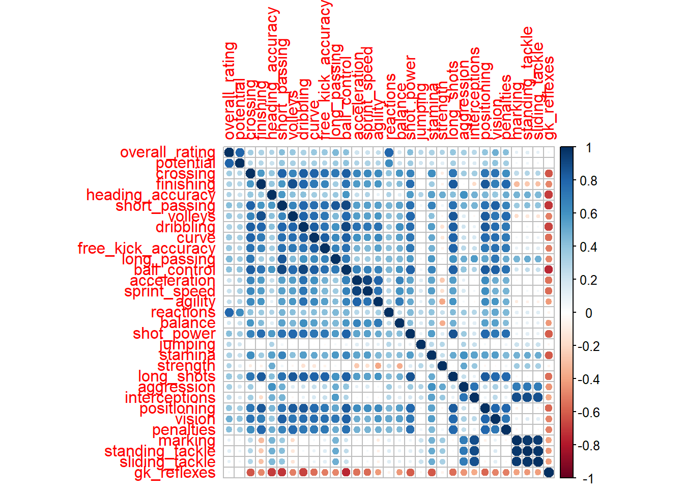
Now that the data is prepared, we can perform a pca analysis. Let’s perform pca with and without rotation. We will use the the raw data, because the principal function uses the correlation matrix to make your principal components and hence should not be scaled. Question: why should this not be scaled?
# Perform Principal Components Analysis (PCA)
pca <- principal(nums, nfactors = 10, rotate = "none")

# Check output
print(pca, sort = TRUE)  #with sort=TRUE, the variables are automatically sorted
## Principal Components Analysis
## Call: principal(r = nums, nfactors = 10, rotate = "none")
## Standardized loadings (pattern matrix) based upon correlation matrix
## item PC1 PC2 PC3 PC4
## ball_control 12 0.95 -0.02 -0.06 -0.06
## short_passing 6 0.91 0.18 -0.06 -0.04
## dribbling 8 0.91 -0.25 -0.14 -0.02
## positioning 25 0.87 -0.27 0.06 -0.14
## long_shots 22 0.87 -0.23 0.08 -0.21
## crossing 3 0.87 0.02 -0.19 0.08
## curve 9 0.86 -0.18 -0.05 -0.03
## vision 26 0.86 -0.08 0.10 -0.02
## shot_power 18 0.85 -0.08 0.13 -0.26
## free_kick_accuracy 10 0.82 -0.10 0.01 -0.11
## volleys 7 0.81 -0.36 0.12 -0.22
## penalties 27 0.80 -0.20 0.19 -0.25
## finishing 4 0.76 -0.48 0.12 -0.27
## long_passing 11 0.75 0.31 -0.02 0.11
## stamina 20 0.72 0.37 -0.11 0.07
## gk_reflexes 31 -0.71 -0.21 0.44 0.29
## acceleration 13 0.71 -0.26 -0.29 0.36
## sprint_speed 14 0.71 -0.20 -0.26 0.30
## agility 15 0.70 -0.36 -0.23 0.40
## balance 17 0.63 -0.16 -0.32 0.40
## heading_accuracy 5 0.58 0.44 0.12 -0.39
## marking 28 0.22 0.92 -0.19 0.06
## standing_tackle 29 0.27 0.91 -0.19 0.05
## sliding_tackle 30 0.25 0.90 -0.22 0.09
## interceptions 24 0.34 0.86 -0.05 0.08
## aggression 23 0.45 0.73 0.09 -0.07
## strength 21 0.03 0.55 0.50 -0.38
## overall_rating 1 0.50 0.12 0.74 0.31
## reactions 16 0.55 0.10 0.61 0.30
## potential 2 0.45 0.01 0.59 0.43
## jumping 19 0.14 0.29 0.26 0.29
## PC5 PC6 PC7 PC8 PC9
## ball_control -0.01 -0.09 -0.10 -0.01 -0.08
## short_passing -0.17 -0.04 -0.10 0.00 -0.18
## dribbling 0.01 -0.09 -0.03 0.04 -0.05
## positioning 0.05 0.03 0.03 -0.12 -0.01
## long_shots -0.08 0.08 0.04 0.07 0.01
## crossing -0.16 -0.02 0.10 0.15 0.05
## curve -0.18 0.05 0.05 0.20 0.12
## vision -0.25 0.13 0.03 -0.14 -0.18
## shot_power 0.07 0.01 0.01 0.05 0.00
## free_kick_accuracy -0.29 0.16 0.05 0.20 0.16
## volleys 0.03 0.04 -0.01 0.02 0.07
## penalties 0.00 0.12 -0.09 -0.11 0.13
## finishing 0.12 0.02 -0.03 -0.04 0.01
## long_passing -0.40 0.07 -0.02 0.06 -0.28
## stamina 0.21 0.00 0.34 -0.10 -0.15
## gk_reflexes -0.22 0.12 0.16 0.03 0.00
## acceleration 0.32 -0.20 0.07 0.05 0.05
## sprint_speed 0.38 -0.26 0.10 0.08 0.04
## agility 0.10 0.04 0.07 0.00 -0.03
## balance 0.04 0.27 -0.13 -0.32 0.07
## heading_accuracy 0.37 -0.09 -0.25 -0.07 0.06
## marking -0.07 -0.03 -0.07 0.03 0.08
## standing_tackle -0.09 -0.02 -0.06 0.03 0.06
## sliding_tackle -0.08 -0.02 -0.06 0.05 0.08
## interceptions -0.14 0.04 0.02 -0.02 0.07
## aggression 0.12 0.06 0.18 -0.17 0.05
## strength 0.30 -0.10 0.23 0.05 -0.10
## overall_rating -0.09 -0.10 -0.03 -0.01 0.03
## reactions -0.06 0.03 0.15 -0.11 0.20
## potential -0.05 -0.32 -0.27 0.03 -0.07
## jumping 0.61 0.52 -0.14 0.24 -0.10
## PC10 h2 u2 com
## ball_control -0.07 0.95 0.0517 1.1
## short_passing -0.06 0.94 0.0629 1.3
## dribbling -0.06 0.92 0.0791 1.3
## positioning -0.08 0.88 0.1192 1.3
## long_shots 0.09 0.89 0.1120 1.4
## crossing -0.07 0.86 0.1377 1.3
## curve -0.01 0.88 0.1244 1.4
## vision -0.05 0.89 0.1131 1.4
## shot_power 0.17 0.85 0.1453 1.4
## free_kick_accuracy 0.12 0.89 0.1071 1.7
## volleys -0.03 0.86 0.1355 1.6
## penalties 0.11 0.83 0.1657 1.7
## finishing -0.04 0.92 0.0818 2.1
## long_passing 0.01 0.92 0.0841 2.3
## stamina -0.04 0.86 0.1415 2.5
## gk_reflexes 0.08 0.93 0.0706 2.8
## acceleration 0.06 0.94 0.0599 3.0
## sprint_speed 0.06 0.93 0.0660 3.0
## agility -0.04 0.85 0.1466 2.5
## balance 0.21 0.94 0.0641 4.1
## heading_accuracy -0.13 0.93 0.0738 4.4
## marking 0.01 0.96 0.0435 1.3
## standing_tackle 0.01 0.96 0.0359 1.3
## sliding_tackle 0.00 0.95 0.0495 1.4
## interceptions -0.03 0.90 0.1023 1.4
## aggression 0.13 0.84 0.1605 2.2
## strength 0.17 0.90 0.1035 4.2
## overall_rating 0.02 0.93 0.0726 2.3
## reactions -0.29 0.94 0.0598 3.6
## potential 0.14 0.94 0.0576 4.1
## jumping -0.06 0.99 0.0068 4.2
##
## PC1 PC2 PC3 PC4 PC5
## SS loadings 14.69 5.59 2.42 1.76 1.44
## Proportion Var 0.47 0.18 0.08 0.06 0.05
## Cumulative Var 0.47 0.65 0.73 0.79 0.84
## Proportion Explained 0.52 0.20 0.09 0.06 0.05
## Cumulative Proportion 0.52 0.72 0.81 0.87 0.92
## PC6 PC7 PC8 PC9 PC10
## SS loadings 0.70 0.50 0.40 0.34 0.32
## Proportion Var 0.02 0.02 0.01 0.01 0.01
## Cumulative Var 0.86 0.87 0.89 0.90 0.91
## Proportion Explained 0.02 0.02 0.01 0.01 0.01
## Cumulative Proportion 0.94 0.96 0.98 0.99 1.00
##
## Mean item complexity = 2.2
## Test of the hypothesis that 10 components are sufficient.
##
## The root mean square of the residuals (RMSR) is 0.01
## with the empirical chi square 1939.19 with prob < 4.6e-282
##
## Fit based upon off diagonal values = 1# based on the highest loadings for the first PC.
# Check the loadings to see what the PCS are about
pca$loadings##
## Loadings:
## PC1 PC2 PC3 PC4
## overall_rating 0.497 0.122 0.741 0.310
## potential 0.448 0.594 0.425
## crossing 0.868 -0.190
## finishing 0.761 -0.485 0.123 -0.265
## heading_accuracy 0.578 0.438 0.120 -0.392
## short_passing 0.910 0.177
## volleys 0.812 -0.361 0.123 -0.223
## dribbling 0.906 -0.249 -0.145
## curve 0.864 -0.182
## free_kick_accuracy 0.822 -0.103 -0.114
## long_passing 0.750 0.308 0.108
## ball_control 0.955
## acceleration 0.712 -0.261 -0.292 0.357
## sprint_speed 0.707 -0.199 -0.256 0.302
## agility 0.702 -0.357 -0.228 0.402
## reactions 0.549 0.104 0.612 0.300
## balance 0.633 -0.164 -0.324 0.399
## shot_power 0.854 0.129 -0.258
## jumping 0.136 0.288 0.264 0.293
## stamina 0.716 0.367 -0.111
## strength 0.555 0.499 -0.380
## long_shots 0.871 -0.230 -0.206
## aggression 0.447 0.727
## interceptions 0.345 0.861
## positioning 0.872 -0.266 -0.141
## vision 0.860
## penalties 0.797 -0.200 0.185 -0.248
## marking 0.219 0.921 -0.193
## standing_tackle 0.273 0.913 -0.188
## sliding_tackle 0.252 0.901 -0.219
## gk_reflexes -0.713 -0.211 0.441 0.291
## PC5 PC6 PC7 PC8
## overall_rating
## potential -0.325 -0.272
## crossing -0.158 0.150
## finishing 0.117
## heading_accuracy 0.371 -0.247
## short_passing -0.165
## volleys
## dribbling
## curve -0.183 0.203
## free_kick_accuracy -0.286 0.164 0.204
## long_passing -0.401
## ball_control
## acceleration 0.315 -0.198
## sprint_speed 0.383 -0.263 0.104
## agility 0.100
## reactions 0.154 -0.111
## balance 0.271 -0.130 -0.322
## shot_power
## jumping 0.613 0.518 -0.145 0.238
## stamina 0.210 0.340 -0.101
## strength 0.300 -0.103 0.225
## long_shots
## aggression 0.115 0.184 -0.171
## interceptions -0.145
## positioning -0.122
## vision -0.248 0.126 -0.135
## penalties 0.115 -0.109
## marking
## standing_tackle
## sliding_tackle
## gk_reflexes -0.221 0.122 0.161
## PC9 PC10
## overall_rating
## potential 0.143
## crossing
## finishing
## heading_accuracy -0.128
## short_passing -0.175
## volleys
## dribbling
## curve 0.115
## free_kick_accuracy 0.163 0.121
## long_passing -0.276
## ball_control
## acceleration
## sprint_speed
## agility
## reactions 0.199 -0.289
## balance 0.210
## shot_power 0.169
## jumping -0.103
## stamina -0.153
## strength -0.103 0.171
## long_shots
## aggression 0.126
## interceptions
## positioning
## vision -0.179
## penalties 0.134 0.106
## marking
## standing_tackle
## sliding_tackle
## gk_reflexes
##
## PC1 PC2 PC3 PC4 PC5
## SS loadings 14.688 5.588 2.425 1.756 1.440
## Proportion Var 0.474 0.180 0.078 0.057 0.046
## Cumulative Var 0.474 0.654 0.732 0.789 0.835
## PC6 PC7 PC8 PC9 PC10
## SS loadings 0.702 0.505 0.401 0.340 0.322
## Proportion Var 0.023 0.016 0.013 0.011 0.010
## Cumulative Var 0.858 0.874 0.887 0.898 0.909We can actually see that the first PC loads high on dribbling, ball_control,long shots, shot_power, vision So we can maybe say that this PC is about ball handling and football intelligence. Looking at PC2, we see that it loads on sliding tackles, interception, and agression, so this can be your defensive skills. As an exercise, try to interpret the other PCs.
# Check the score to see which instances score high on
# certain PCs
head(pca$scores)
## PC1 PC2 PC3 PC4
## [1,] -0.3916228 0.7864349 -0.9646160 -1.04977239
## [2,] 0.5358301 0.4865027 -0.9412600 1.77302473
## [3,] 0.5546452 -0.9598542 -0.4630592 0.09590248
## [4,] -0.3624813 1.3420597 0.2677645 -0.84453112
## [5,] -0.3246658 1.7466316 0.7398201 0.29588598
## [6,] 1.4602375 -0.8321987 1.2660571 0.33471345
## PC5 PC6 PC7 PC8
## [1,] -0.1857767 -0.5709827 -1.2941700 -0.2079504
## [2,] -0.1457836 1.1401279 -0.4622942 0.4218186
## [3,] 0.5638614 0.2841281 0.1767969 -0.2646224
## [4,] -0.3313796 -0.3017848 -1.1603707 1.7917709
## [5,] 0.2321783 0.3631449 -1.9867849 -0.8659367
## [6,] -0.3264924 0.1431034 0.1072922 0.2416088
## PC9 PC10
## [1,] -0.791041954 1.7251407
## [2,] 1.288064235 0.7615998
## [3,] -2.230868898 2.4339190
## [4,] -1.274688621 -0.8312371
## [5,] 0.179336223 -1.5820336
## [6,] 0.008017534 -0.8480305# How many PCs to keep? Check eigenvalues We should go for
# 5 in this case
pca$values #based on Kaiser criterion: eigenvalues > 1## [1] 14.68817338 5.58781625 2.42484785
## [4] 1.75561797 1.44033982 0.70155485
## [7] 0.50497148 0.40075652 0.33988059
## [10] 0.32209933 0.26697913 0.25997298
## [13] 0.23301811 0.22980121 0.21847876
## [16] 0.18690795 0.16991019 0.15128742
## [19] 0.14675786 0.13845947 0.11959460
## [22] 0.11392462 0.10610977 0.10095204
## [25] 0.08096761 0.07461259 0.06823503
## [28] 0.06325777 0.04192702 0.03764140
## [31] 0.02514642# Make Cattell's Scree plot of eigenvalues This makes us
# choose for 5 or 6
plot(pca$values, type = "b", ylab = "Eigenvalues", xlab = "Number of Principal Components",
main = "Cattell's Scree plot")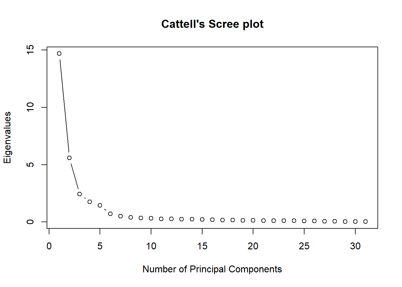
# Check cumulative PVE We want at least 70%, so we could go
# for 3
cumsum(prop.table(pca$values))
## [1] 0.4738120 0.6540642 0.7322851 0.7889179
## [5] 0.8353805 0.8580113 0.8743007 0.8872283
## [9] 0.8981922 0.9085825 0.9171947 0.9255810
## [13] 0.9330977 0.9405106 0.9475583 0.9535876
## [17] 0.9590686 0.9639488 0.9686830 0.9731494
## [21] 0.9770073 0.9806823 0.9841052 0.9873617
## [25] 0.9899735 0.9923804 0.9945815 0.9966221
## [29] 0.9979746 0.9991888 1.0000000# Plot cumulative PVE Not so clear cut, maybe 4 or 5
plot(cumsum(prop.table(pca$values)), type = "b", ylab = "Cumulative Proportion of Variance Explained (%)",
xlab = "Number of Principal Components", main = "Selecting the optimal number of PCs")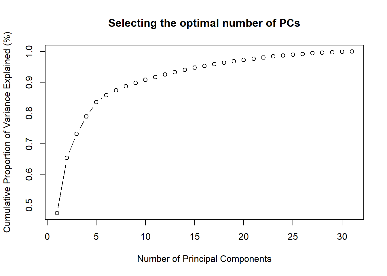
# MORE ADVANCED METHODS

# Horn's Parallel Analysis By default, fa.parallel takes
# the mean of the eigenvalues of the random matrices.  By
# specifying quant=0.95, the 95th percentile (as originally
# in Horn (1965)) are used instead.
hpa <- fa.parallel(x = nums, fm = "ml", fa = "pc", n.iter = 50)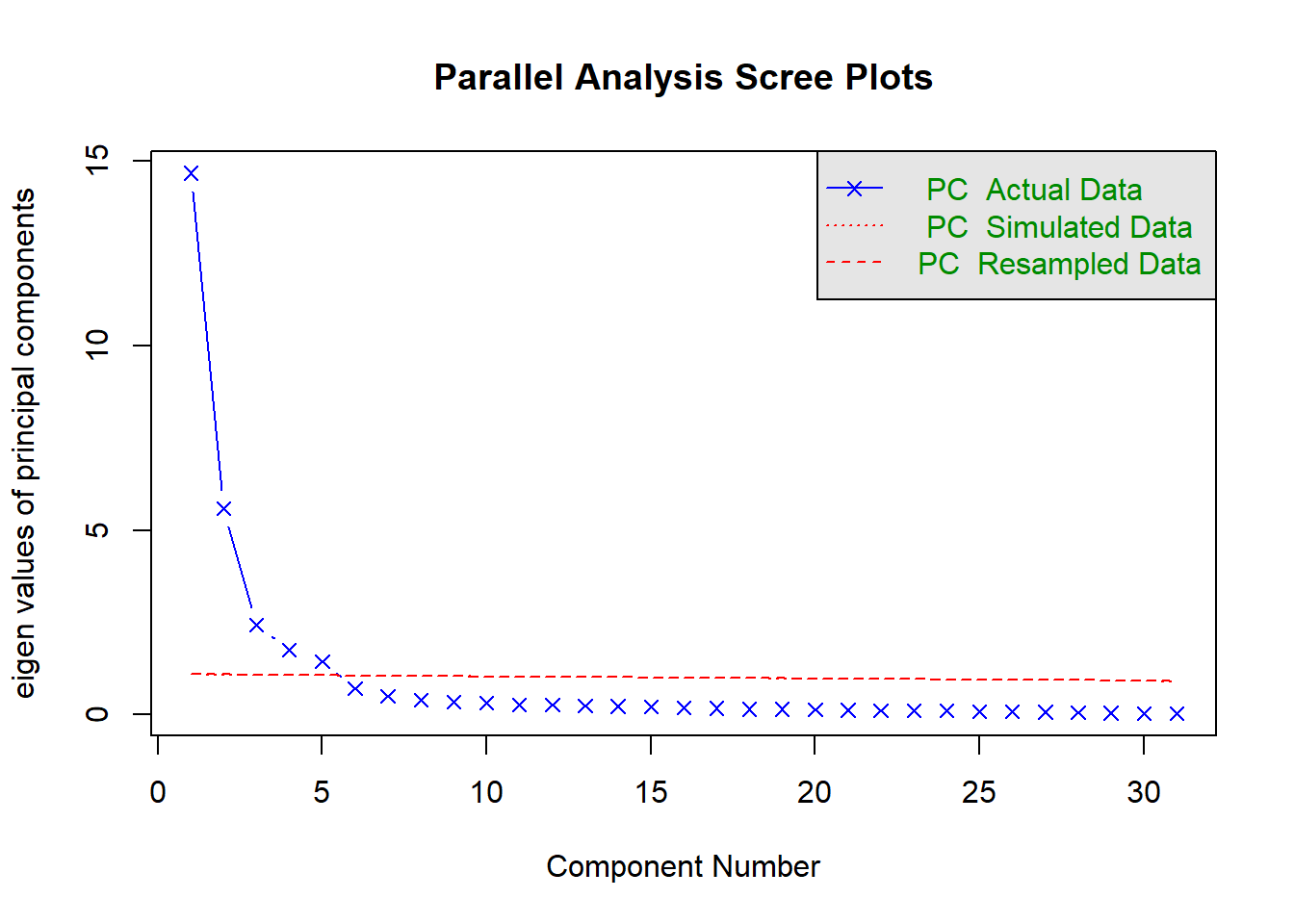
## Parallel analysis suggests that the number of factors = NA and the number of components = 5Since most methods give around approximately around 5 PCs, 5 PCs would be a good final choice. It is always advisable to try out different methods and check for consistency. Remember that you can also apply a varimax rotation to increase interpretabiliy.
# Rotations
pca2 <- principal(nums, nfactors = 5, rotate = "varimax")

# Check interpretation You can see that the the first PC is
# now clearly ball handling or even striking skills
# Especially PC2 is more clear since it loads very high on
# marking and tackles, which are defensive skills
pca2$loadings
##
## Loadings:
## RC1 RC2 RC4 RC3
## overall_rating 0.294 0.119 0.893
## potential 0.215 0.152 0.814
## crossing 0.706 0.329 0.422 0.124
## finishing 0.870 -0.293 0.197
## heading_accuracy 0.514 0.462
## short_passing 0.767 0.453 0.254 0.180
## volleys 0.876 -0.150 0.188 0.144
## dribbling 0.829 0.458
## curve 0.810 0.110 0.313 0.168
## free_kick_accuracy 0.811 0.170 0.159 0.178
## long_passing 0.566 0.564 0.168 0.297
## ball_control 0.837 0.263 0.357 0.142
## acceleration 0.446 0.819
## sprint_speed 0.444 0.772
## agility 0.473 0.762 0.161
## reactions 0.337 0.140 0.792
## balance 0.374 0.113 0.718
## shot_power 0.855 0.110 0.130 0.152
## jumping -0.163 0.170 0.270 0.320
## stamina 0.452 0.534 0.364 0.105
## strength 0.343 -0.506 0.188
## long_shots 0.900 0.179 0.156
## aggression 0.221 0.754 0.169
## interceptions 0.927 0.157
## positioning 0.861 0.285 0.153
## vision 0.794 0.185 0.199 0.304
## penalties 0.842 0.191
## marking 0.966
## standing_tackle 0.975
## sliding_tackle 0.966
## gk_reflexes -0.634 -0.441 -0.318 0.359
## RC5
## overall_rating 0.129
## potential
## crossing -0.148
## finishing 0.157
## heading_accuracy 0.591
## short_passing
## volleys
## dribbling
## curve -0.148
## free_kick_accuracy -0.191
## long_passing -0.274
## ball_control
## acceleration 0.119
## sprint_speed 0.216
## agility
## reactions 0.119
## balance -0.133
## shot_power 0.203
## jumping 0.635
## stamina 0.272
## strength 0.618
## long_shots
## aggression 0.329
## interceptions
## positioning 0.102
## vision -0.142
## penalties 0.128
## marking
## standing_tackle
## sliding_tackle
## gk_reflexes -0.234
##
## RC1 RC2 RC4 RC3 RC5
## SS loadings 11.217 6.038 3.945 2.907 1.790
## Proportion Var 0.362 0.195 0.127 0.094 0.058
## Cumulative Var 0.362 0.557 0.684 0.778 0.835# Make a biplot to check the differences between rotation
# and no rotation Do make good biplot, only select the
# first two PCs
pca <- principal(nums, nfactors = 2, rotate = "none")
pca2 <- principal(nums, nfactors = 2, rotate = "varimax")
biplot(pca)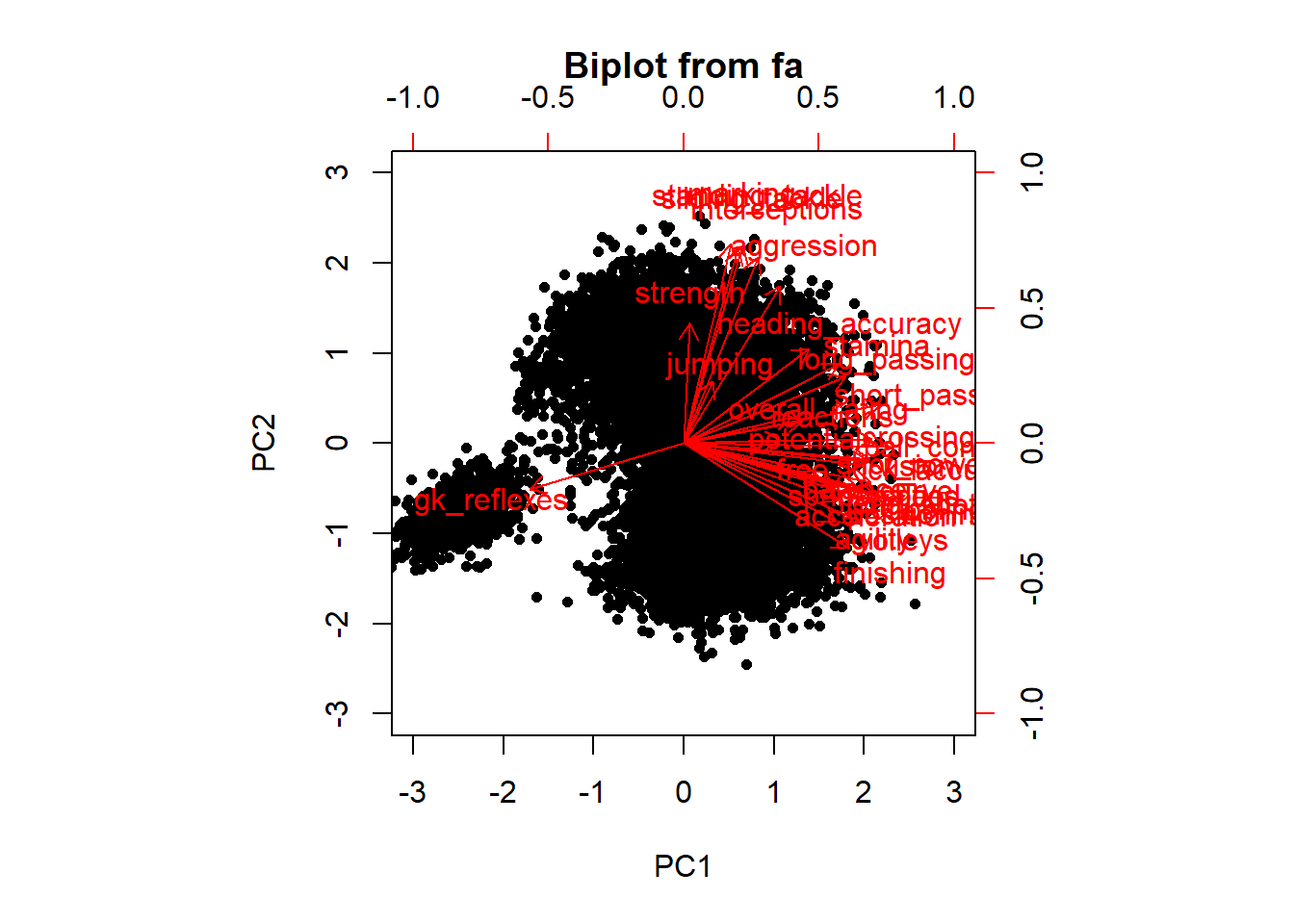
biplot(pca2)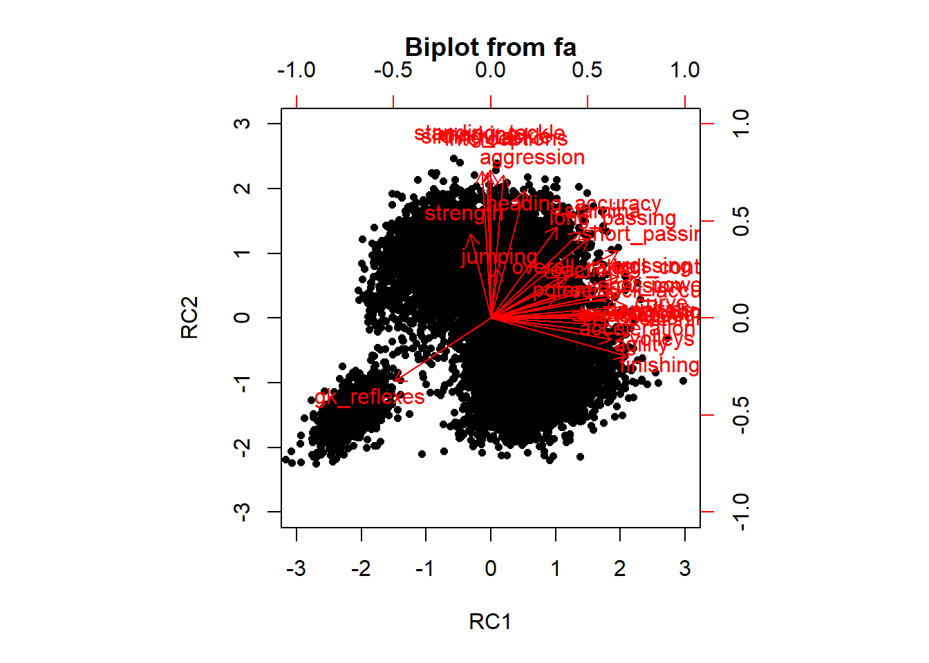
If there are nonlinear relationhsip, it can be good to also try out kernel PCA. If you do not have a response variable, it is of course hard to tell whether there are nonlinearities in the data. Let’s make a synthetic data set to show the power of kpca when the data in highly nonlinear.
# Load the following github directory to make a special
# data set
p_load_current_gh("elbamos/clusteringdatasets")

# Make moons data set
synt <- data.frame(make_moons(n_samples = 1000, noise = 0.02))

ggplot(synt, aes(samples.1, samples.2, col = as.factor(labels))) +
    geom_point()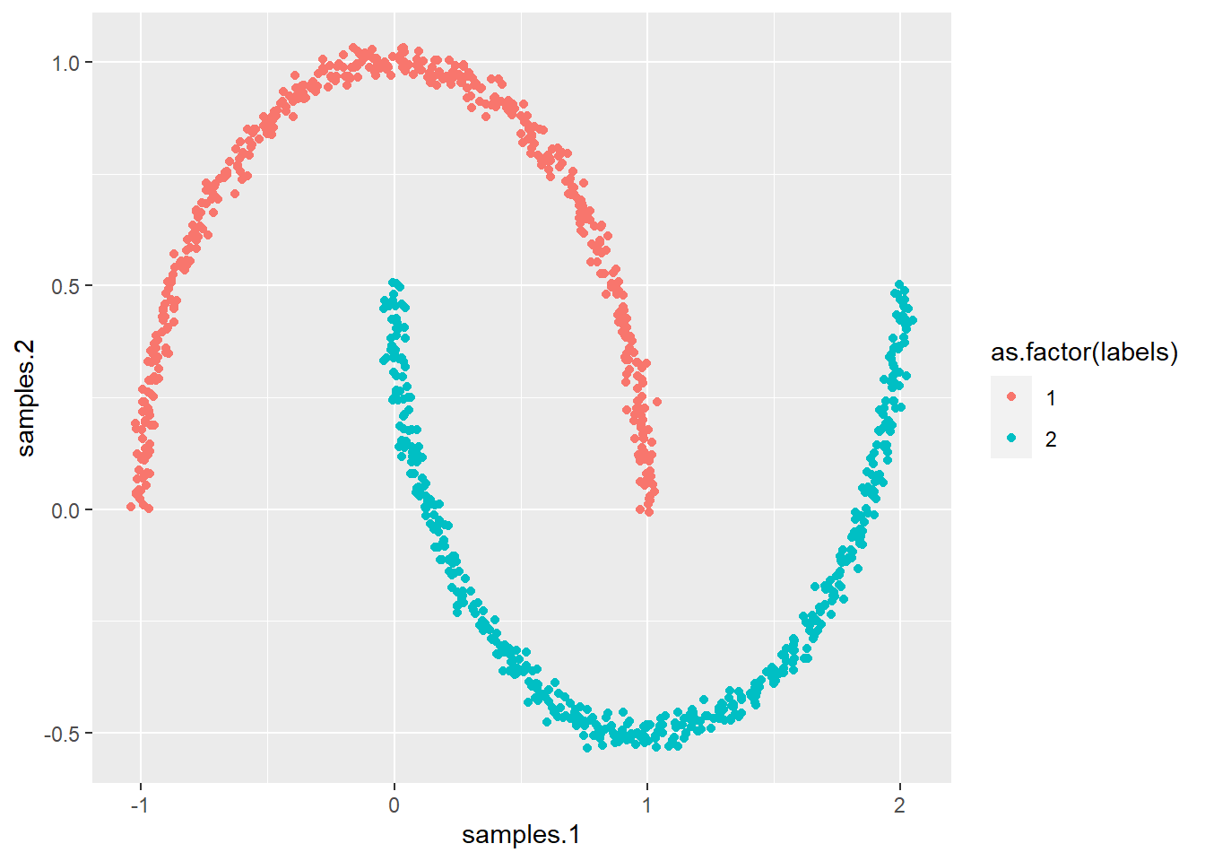
# As you can see this data is no lineary separable So let's
# perform PCA and see what happens As you can see the data
# is no linearly separable
pca3 <- principal(synt[, 1:2], nfactors = 2, rotate = "varimax")
scores <- as.data.frame(cbind(pca3$scores, synt$labels))
ggplot(scores, aes(RC1, RC2, col = as.factor(V3))) + geom_point()
# Perform kernel PCA

# As you can see that the data is now linearly separable
# Note that this is highly dependent upon your choice for
# sigma
p_load(kernlab)
pcak <- kpca(data.matrix(synt[, 1:2]), kernel = "rbfdot", kpar = list(sigma = 15),
    features = 2)

# Plot the scores for kPC2 and kPC2
scoresk <- as.data.frame(cbind(rotated(pcak), synt$labels))
ggplot(scoresk, aes(V1, V2, col = as.factor(V3))) + geom_point()
8.2 Clustering
Clustering is often used in market segmentation and can be very handy to get more insight into your target population. Recall that there are two broad categories: hierarchical and nonhierarchical methods.
We will not discuss all the distance metrics in detail but mention them along the road.
8.2.1 Partitional clustering
Probably the most popular partitional clustering method is k-means. The algorithm is simple and intuitive and works well in a lot of cases. Recall that k-means works with Euclidean distances, so scaling the data is crucial.K-means is built in R by default in the stats package, so we don’t need to load any other packages.
#We will just use the football data set to see whether we can come up with a
#good clustering solution

#Cluster the scaled dataset in 4 groups (one for each position:
#goalie, defender, midfielder and attacker)
km <- kmeans(x=football_sc,
             centers=4,
             nstart=50)

#Plot
plot(x=football_sc,
     col=(km$cluster+1),
     pch = 20 ,
     cex = 1.5,main="k-means clustering")
points(km$centers, col = 2:max(km$cluster+1),cex=5,pch=10) 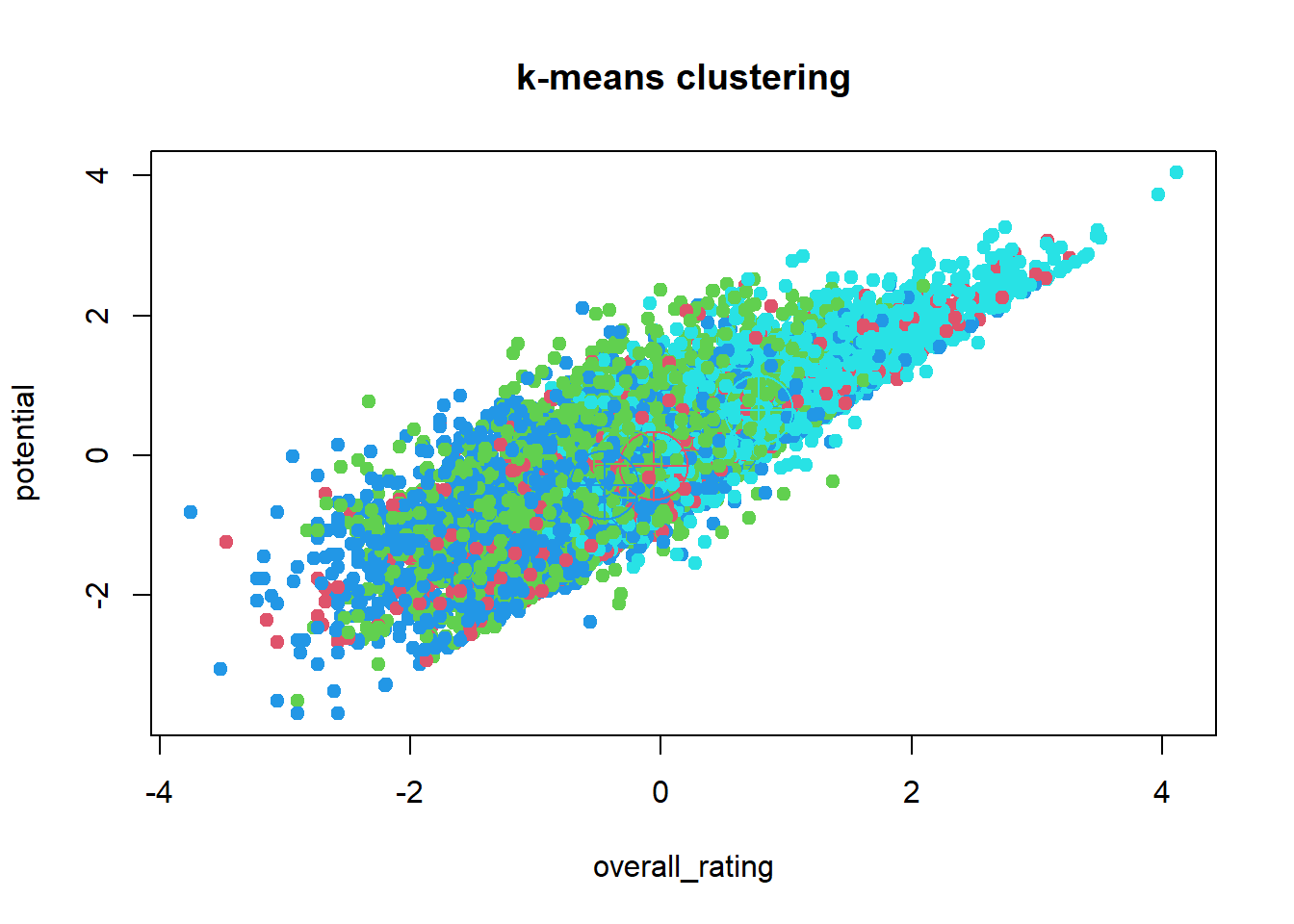
#adds the center, although not clear

#To make a cluster plot based on the PCs, use the cluster package
p_load(cluster)
clusplot(x=football_sc, clus= km$cluster, shade=TRUE, color= TRUE, lines = 0)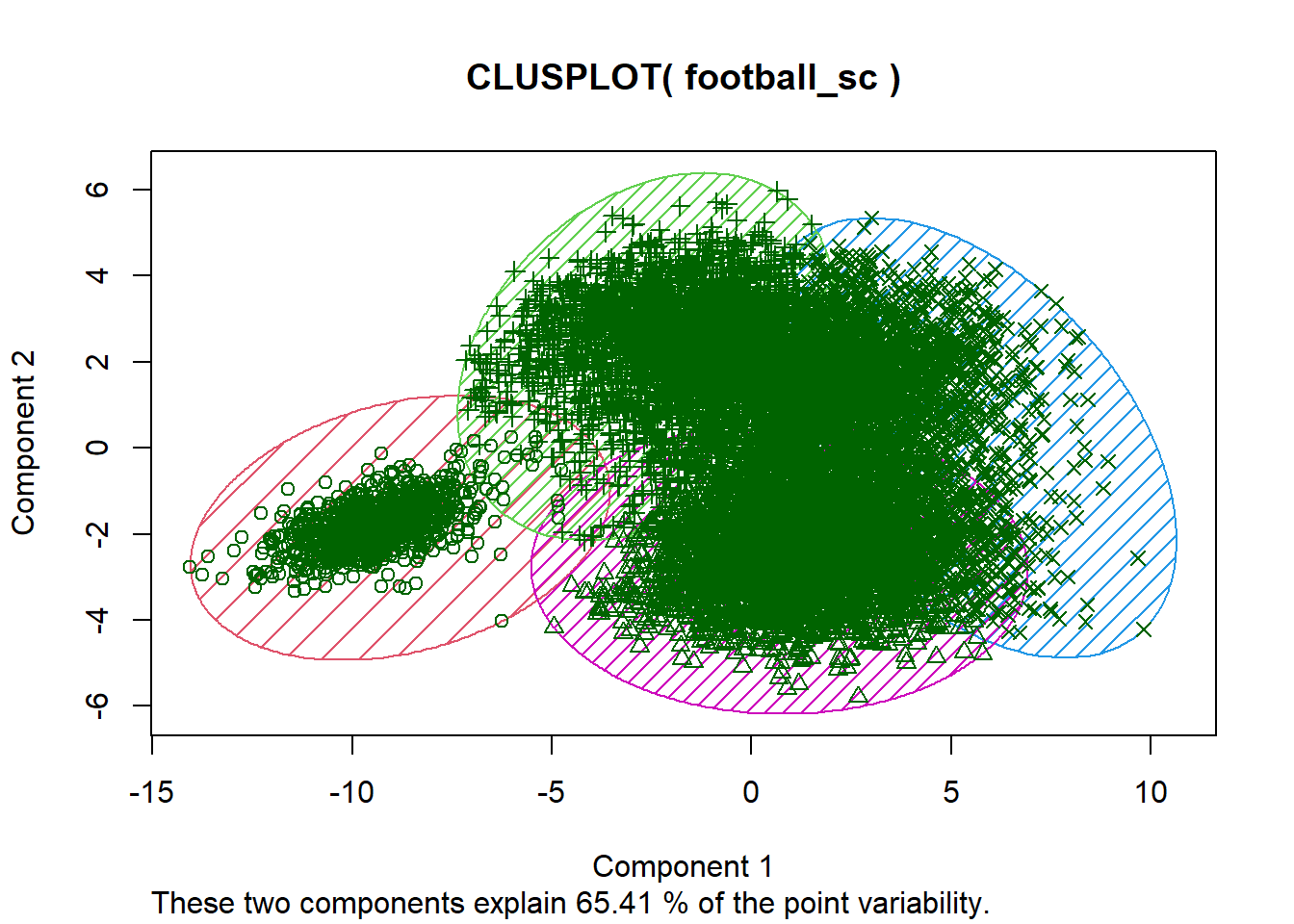
#An even nicer plot package is the fviz_cluster function of the factoextra package
#This use a ggplot style theme
p_load(factoextra)

fviz_cluster(km, data = football_sc,
             geom = "point",
             ellipse.type = "convex")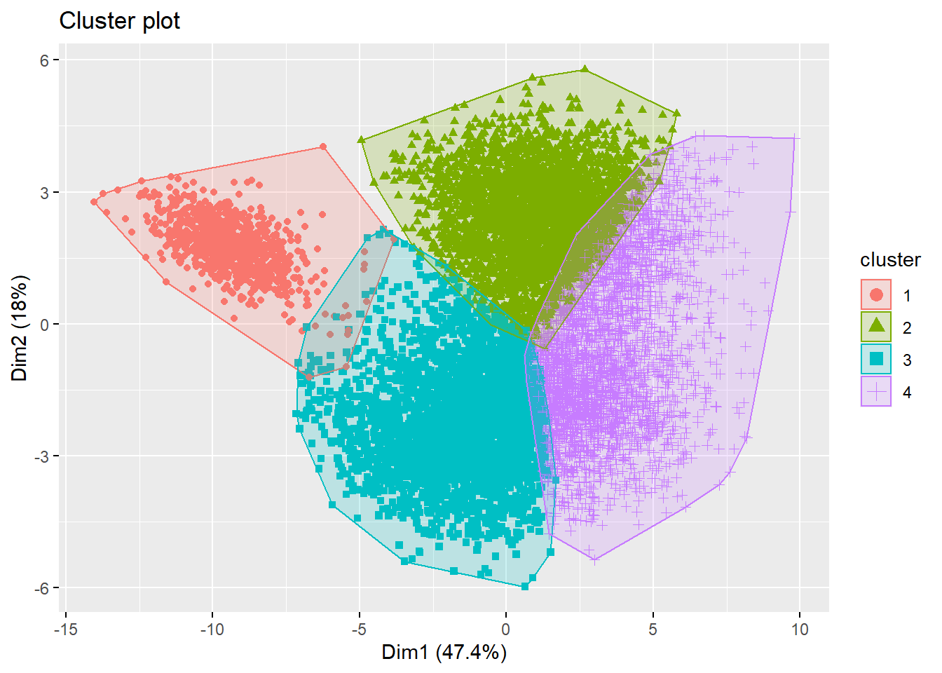
We have succesfully created clusters, however how do we know what all these clusters mean? A good solution can be to build a decision tree with the clusters as a dependent variable and the others as independent.
p_load(rpart)
p_load(rpart.plot)

# Use the unscaled data for better interpretation Can you
# guess the interpretation of each cluster?
tree_data <- data.frame(nums, cluster = as.factor(km$cluster))
dt <- rpart(cluster ~ ., tree_data)
rpart.plot(dt)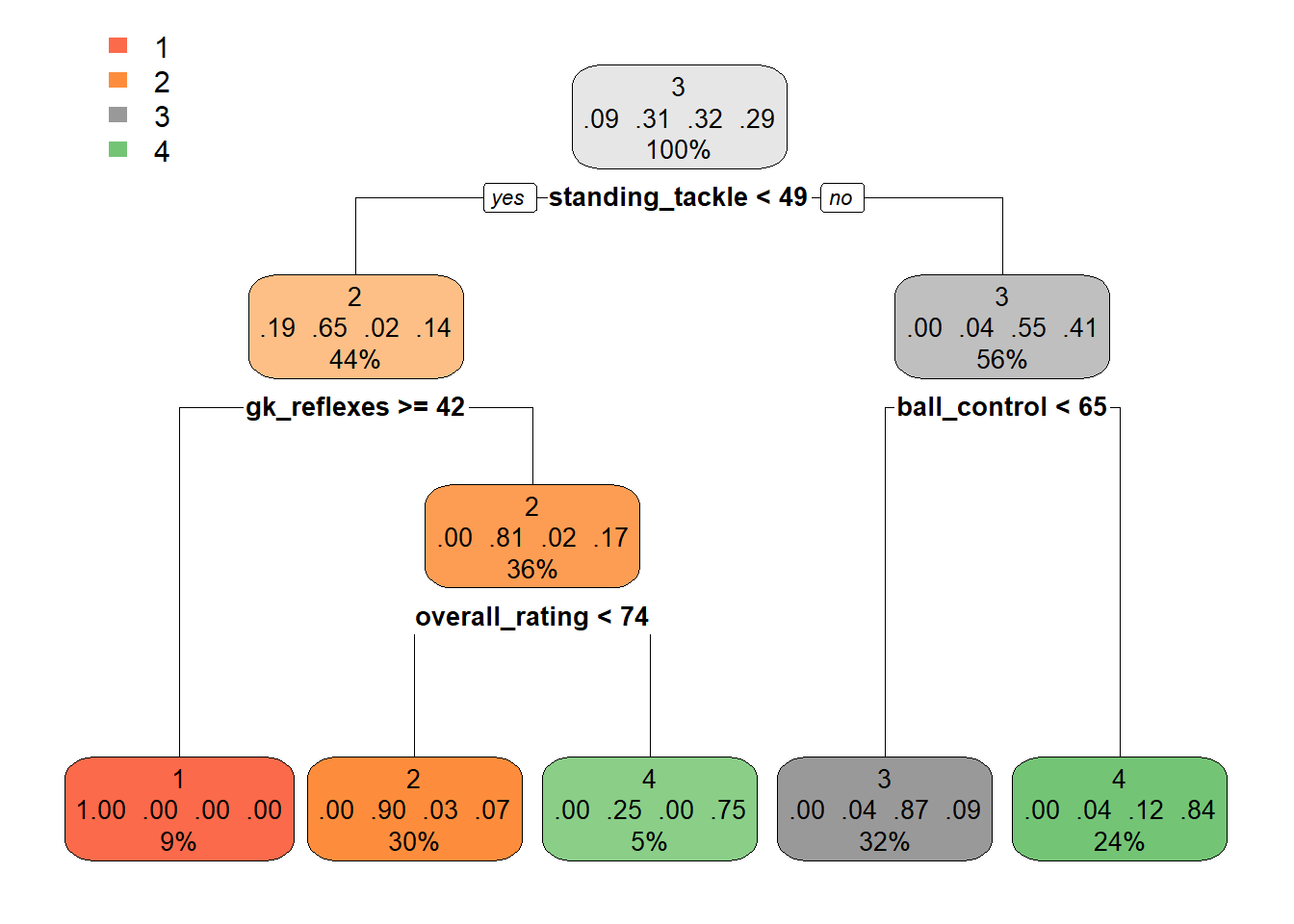
# You can also just have a look at the mean scores per
# cluster Can you guess the interpration now?
tree_data %>%
    group_by(cluster) %>%
    summarise_all(mean)
## # A tibble: 4 x 32
## cluster overall_rating potential crossing
## <fct> <dbl> <dbl> <dbl>
## 1 1 66.5 71.2 18.9
## 2 2 65.2 71.4 54.9
## 3 3 64.1 69.7 48.1
## 4 4 71.7 75.8 66.3
## # ... with 28 more variables: finishing <dbl>,
## # heading_accuracy <dbl>, short_passing <dbl>,
## # volleys <dbl>, dribbling <dbl>, curve <dbl>,
## # free_kick_accuracy <dbl>, long_passing <dbl>,
## # ball_control <dbl>, acceleration <dbl>,
## # sprint_speed <dbl>, agility <dbl>,
## # reactions <dbl>, balance <dbl>, ...Whereas k-means uses the Euclidean distance by default, k-medoids allows you to set the distance measure yourself. Because the cluster center in the case of k-medoids is also a true data point (and not a fictional as in k-means), it can easily work with any type of data. To calculate the distances, you can just use the dist function of the stats package, check ?dist to see the various options.
# To implement kmedoids we use the cluster package
p_load(cluster)

# Use a random subsample becasue distance measures can
# takje a while
random <- sample(1:nrow(nums), 1000, replace = FALSE)

# Calculate dissimilarity matrix with cityblock distance
ds <- stats::dist(football_sc[random, ], method = "manhattan")

# Perform k-medoids
kmd <- pam(x = ds, k = 4, diss = TRUE)  #diss=TRUE means we supply a dissimilarity matrix to x

# Plot
clusplot(x = football_sc[random, ], clus = kmd$cluster, shade = TRUE,
    color = TRUE, lines = 0)
# Have a look at the medoids What is the difference?
nums[random, ][kmd$medoids, ] %>%
    as_tibble()
## # A tibble: 4 x 31
## overall_rating potential crossing finishing
## <dbl> <dbl> <dbl> <dbl>
## 1 64.3 74.1 63.3 64
## 2 63.9 67.7 58.4 32
## 3 70.8 74.3 66.7 60.6
## 4 65.2 75.2 22 17.7
## # ... with 27 more variables:
## # heading_accuracy <dbl>, short_passing <dbl>,
## # volleys <dbl>, dribbling <dbl>, curve <dbl>,
## # free_kick_accuracy <dbl>, long_passing <dbl>,
## # ball_control <dbl>, acceleration <dbl>,
## # sprint_speed <dbl>, agility <dbl>,
## # reactions <dbl>, balance <dbl>, ...As an exercise you can also build a decision tree and see what this says about the clusters.
8.2.2 Hierarchical clustering
One of the downsides of partitional clustering is that you have to specificy the clusters upfront. Hierarchical clustering solves this issue and allows you to make the ‘cut’ yourself. We will focus on agglomorative clustering which applies a bootum-up approach.
Again, hierarchical clustering is included in the stats package of R, so no need to load a new package.
# Calculate dissimilarity
ds <- stats::dist(football_sc, method = "euclidean")

# Perform Hierarchical clustering with ward's method (you
# can experiment with others as well)
hclustering <- hclust(ds, method = "ward.D")

# Plot the dendogram
plot(hclustering)
abline(h = 3000, col = "red", lwd = 3)
# plot a red line across the dendrogram, which gives you 4
# clusters

# Show the 4 clusters
plot(hclustering, cex = 0.6)
rect.hclust(hclustering, k = 4, border = 2:5)
# Cut the tree
cluster_memberships <- cutree(hclustering, 7)

# We can also plot the total distance against the number of
# clusters and look for a elbow The elbow is around 3 or 5
data.frame(distance = hclustering$height, clusters = cluster_memberships[-1]) %>%
    group_by(clusters) %>%
    dplyr::summarise(means = sum(distance)) %>%
    mutate(cumul = cumsum(means)) %>%
    ggplot(aes(clusters, cumul)) + geom_line()
# So let's keep it in the middle and pick 4 just like
# before
cluster_memberships <- cutree(hclustering, 4)

# Plot the cluster memberships
fviz_cluster(list(data = football_sc, cluster = cluster_memberships),
    geom = "point", ellipse.type = "convex")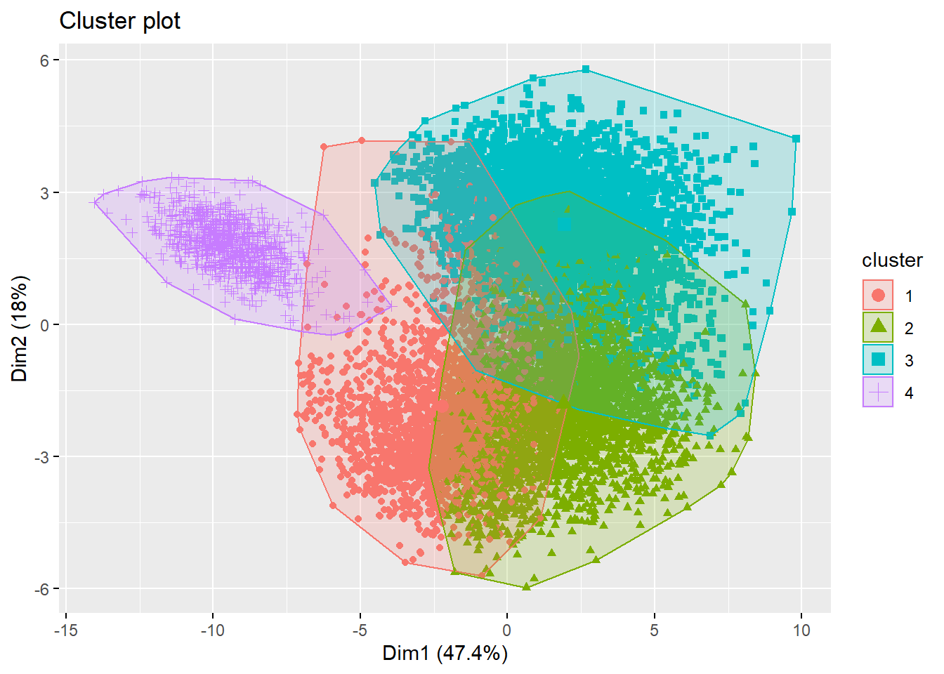
8.2.3 Advanced clustering
Whern the data is highly nonlinear, the traditional methods like k-means or k-medoids often fall short. The main reason for this is because these traditional methods are based on compactness and not on connectivity. To make the example more clear, we will use the moon data example again from kernel PCA and perform k-means, spectral clustering and DBSCAN.
# Remember the moon data
ggplot(synt, aes(samples.1, samples.2, col = as.factor(labels))) +
    geom_point()
# Using Kmeans on this example would give us As you can
# see, this is not really what we want
km_synt <- kmeans(x = synt[, 1:2], centers = 2, nstart = 50)

ggplot(synt, aes(samples.1, samples.2, col = as.factor(km_synt$cluster))) +
    geom_point()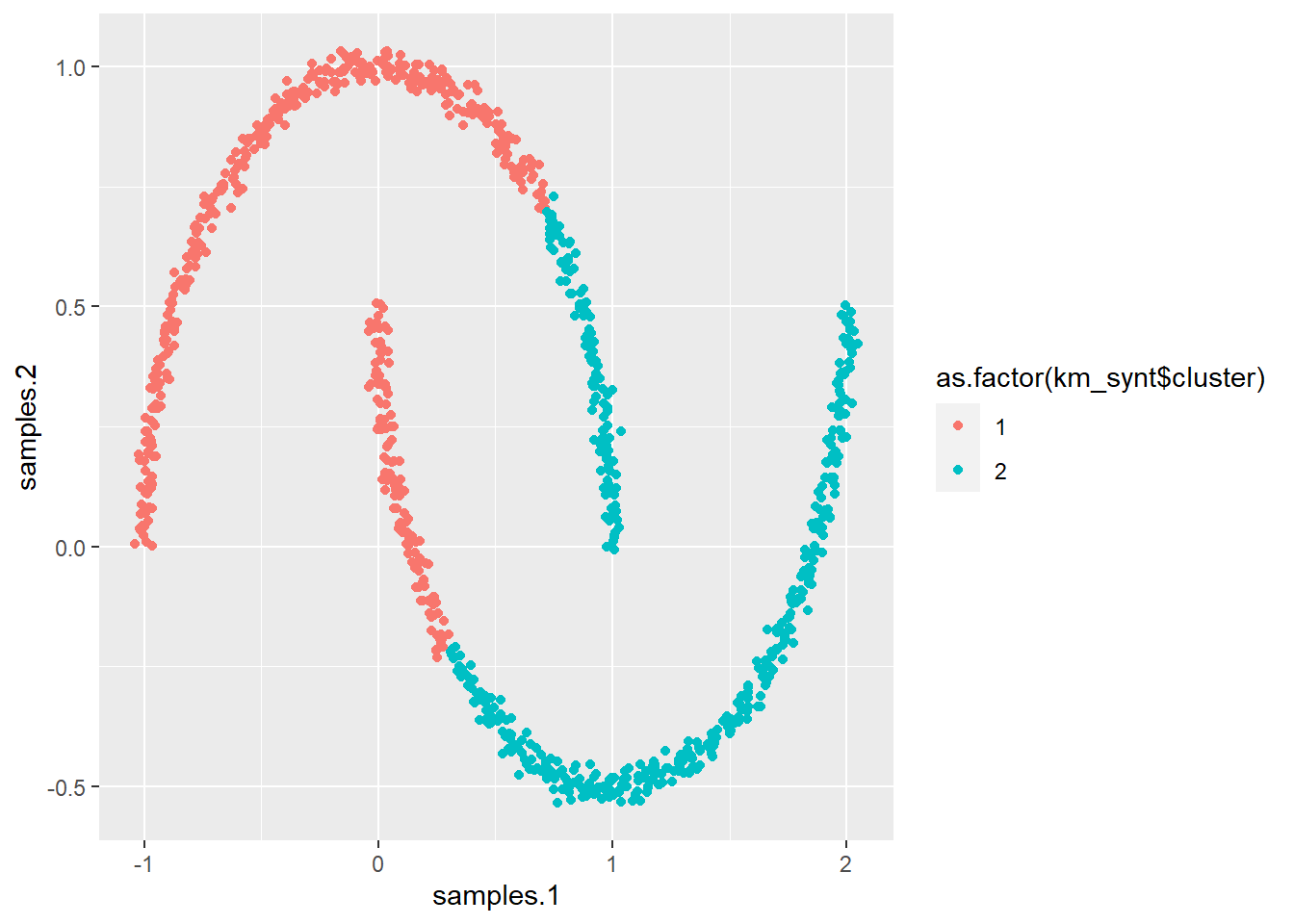
# Let's try spectral clustering We can just use the kernel
# package from kernel PCA
specc_synt <- specc(x = data.matrix(synt[, 1:2]), centers = 2,
    iterations = 200, kernel = "rbfdot", kpar = list(sigma = 15))

# also an option to chose kpar automatically

# If we plot this you nicely see that this is the solution
# that we want
ggplot(synt, aes(samples.1, samples.2, col = as.factor(specc_synt@.Data))) +
    geom_point()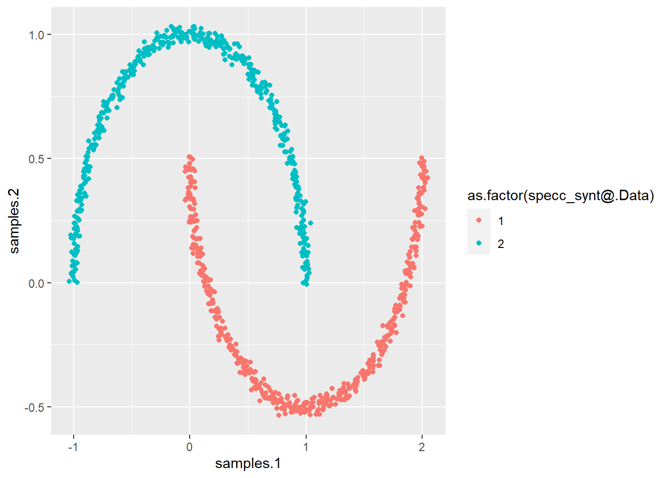
# Let us now do the same with DBSCAN
p_load(dbscan)

# Note that in DBSCAN you should not even set the number of
# clusters!
db_synt <- dbscan(synt[, 1:2], eps = 0.15)

# And plot it ...
ggplot(synt, aes(samples.1, samples.2, col = as.factor(db_synt$cluster))) +
    geom_point()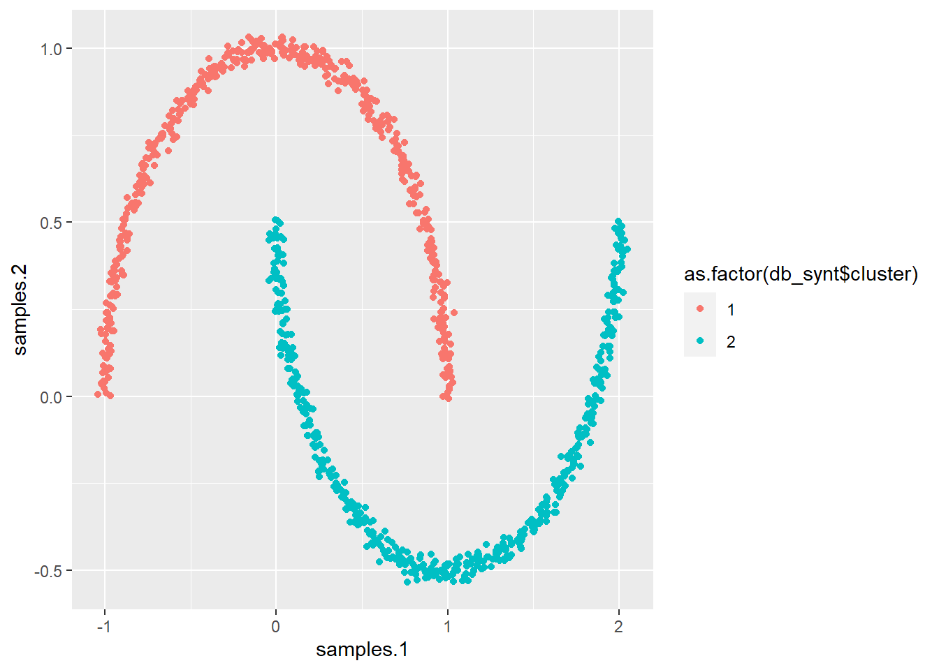
# Let's try another dataset for fun
data("face")
qplot(x = face$x, y = face$y)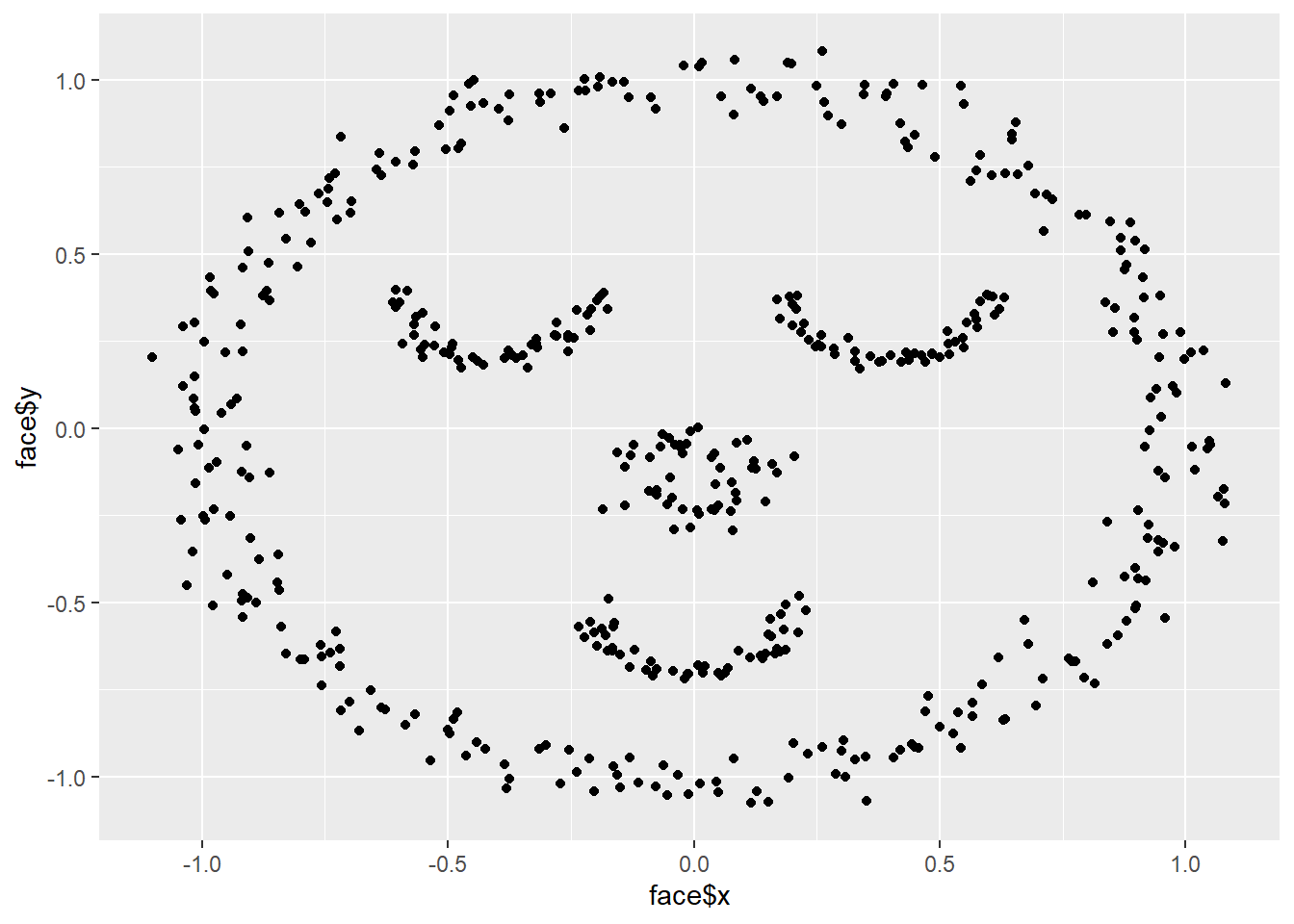
# Spectral
specc_face <- specc(x = data.matrix(face), centers = 5, iterations = 200,
    kernel = "rbfdot")
ggplot(face, aes(x, y, col = as.factor(specc_face@.Data))) +
    geom_point()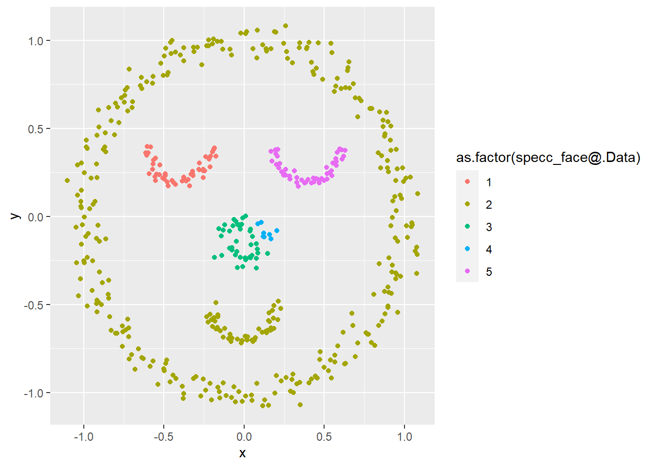
# DBSCAN
db_face <- dbscan(face, eps = 0.15)
ggplot(face, aes(x, y, col = as.factor(db_face$cluster))) + geom_point()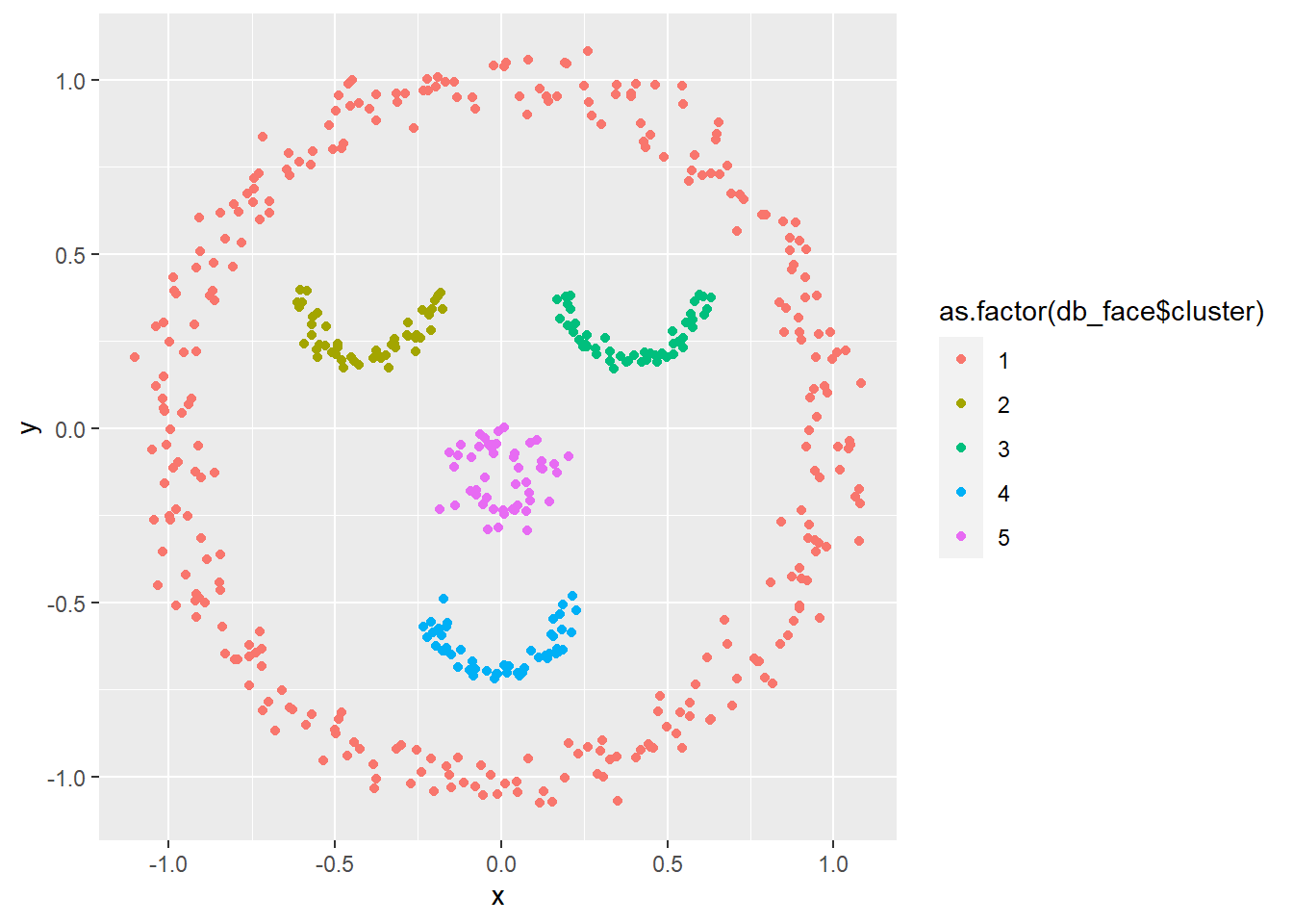
8.2.4 Cluster evaluation
The question now of course arises: how to pick the best clustering solution. We have tried out several methods, however, we should know which one to pick. In theory, we proposed several methods: silhouette index, Davies-Bouldin index, and the Dunn index. A decision tree can also be build (cf. supra), however this is mainly good for interpretation purposes.
# Lets rebuild our football cluster for kmeans Since we
# don't know the optimal number, let's make a loop and
# decide upon the aforementioned metrics Check cluster
# validity for multiple values of k
kms <- list()
for (k in 2:6) {
    kms[[k]] <- kmeans(x = football_sc, centers = k, nstart = 50)
}

kms[[1]] <- NULL

# Silhouette index (maximize)
ds <- dist(football_sc, method = "euclidean")
sapply(kms, function(km) summary(silhouette(km$cluster, ds))$avg.width)
## [1] 0.4286009 0.2482518 0.2307827 0.2111661
## [5] 0.1759047# Dunn index (maximize)
p_load(clValid)
sapply(kms, function(km) dunn(ds, km$cluster))## [1] 0.08765093 0.09559838 0.09472543 0.02668480
## [5] 0.08928985# Davies-Bouldin index (minimize)
p_load(clusterSim)
sapply(kms, function(km) index.DB(football_sc, km$cluster)$DB)## [1] 0.9744974 1.3988414 1.4341121 1.4800272
## [5] 1.6716166# Choose optimal number of clusters k using all cluster
# validation measures (24 measures)
p_load(NbClust)
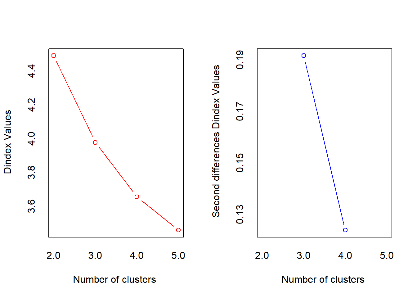
nbc <- NbClust(data = football_sc[random, ], min.nc = 2, max.nc = 5,
method = "kmeans", index = "all")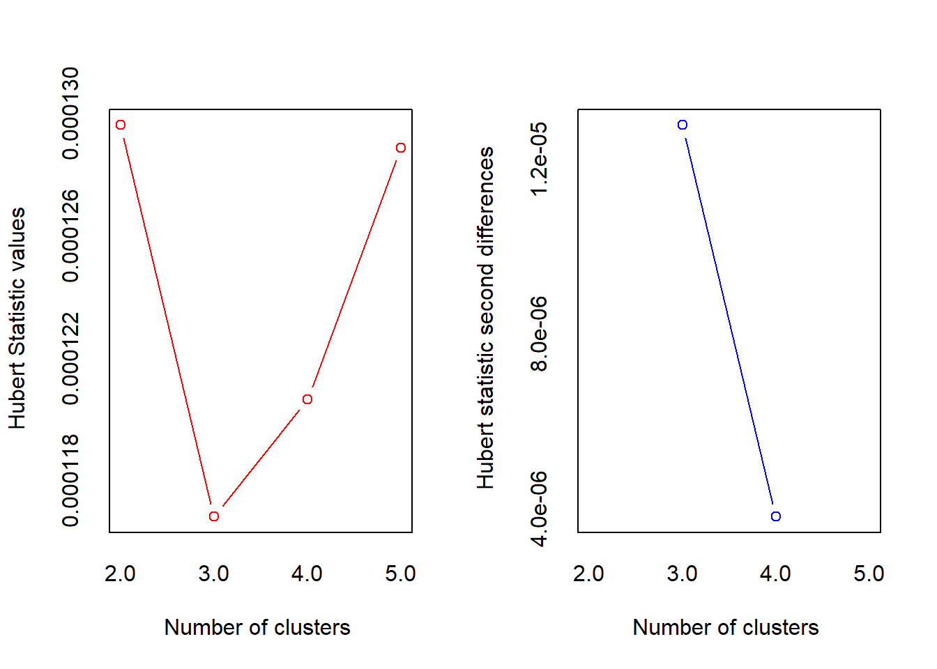
## *** : The Hubert index is a graphical method of determining the number of clusters.
##                 In the plot of Hubert index, we seek a significant knee that corresponds to a
##                 significant increase of the value of the measure i.e the significant peak in Hubert
##                 index second differences plot.
## 
## *** : The D index is a graphical method of determining the number of clusters.
## In the plot of D index, we seek a significant knee (the significant peak in Dindex
## second differences plot) that corresponds to a significant increase of the value of
## the measure.
##
## *******************************************************************
## * Among all indices:
## * 8 proposed 2 as the best number of clusters
## * 11 proposed 3 as the best number of clusters
## * 2 proposed 4 as the best number of clusters
## * 3 proposed 5 as the best number of clusters
##
## ***** Conclusion *****
##
## * According to the majority rule, the best number of clusters is 3
##
##
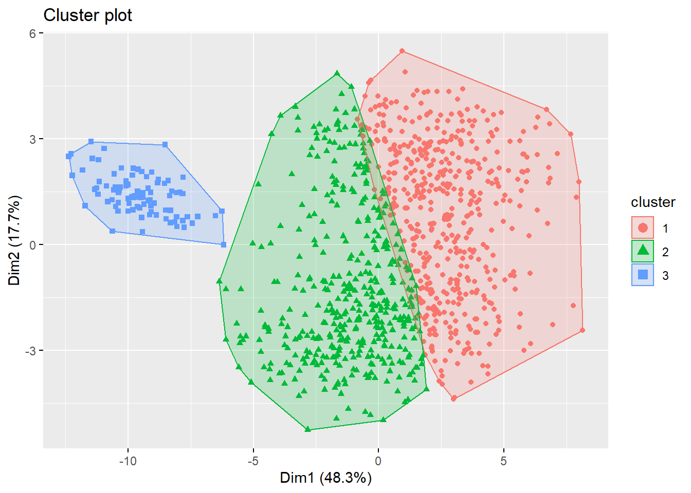
## *******************************************************************# Plot, optimal number of clusters was suggested as 3
fviz_cluster(list(data = football_sc, cluster = kms[[2]]$cluster),
geom = "point", ellipse.type = "convex")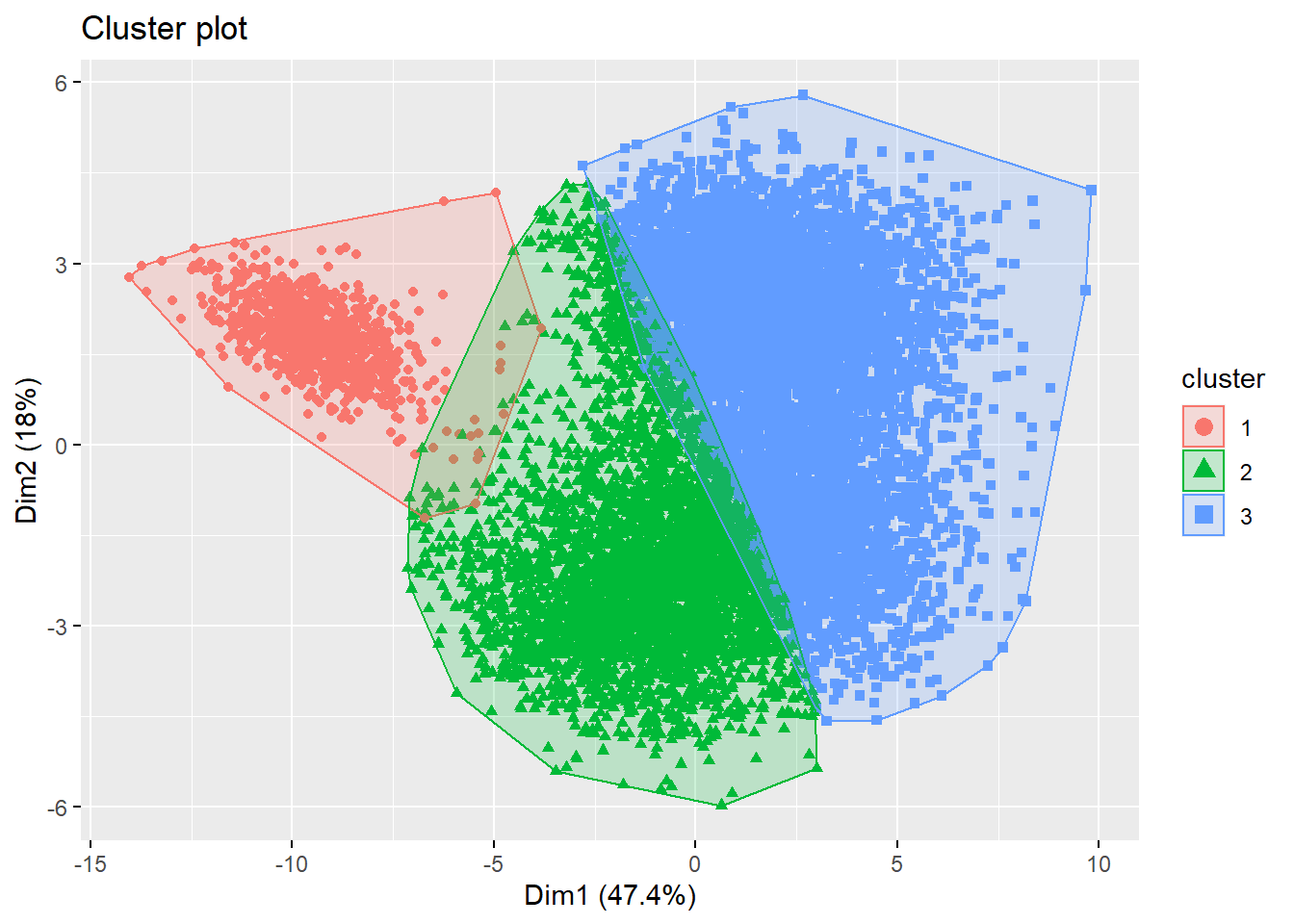
# Also much evidence for 2: compare
fviz_cluster(list(data = football_sc, cluster = kms[[1]]$cluster),
geom = "point", ellipse.type = "convex")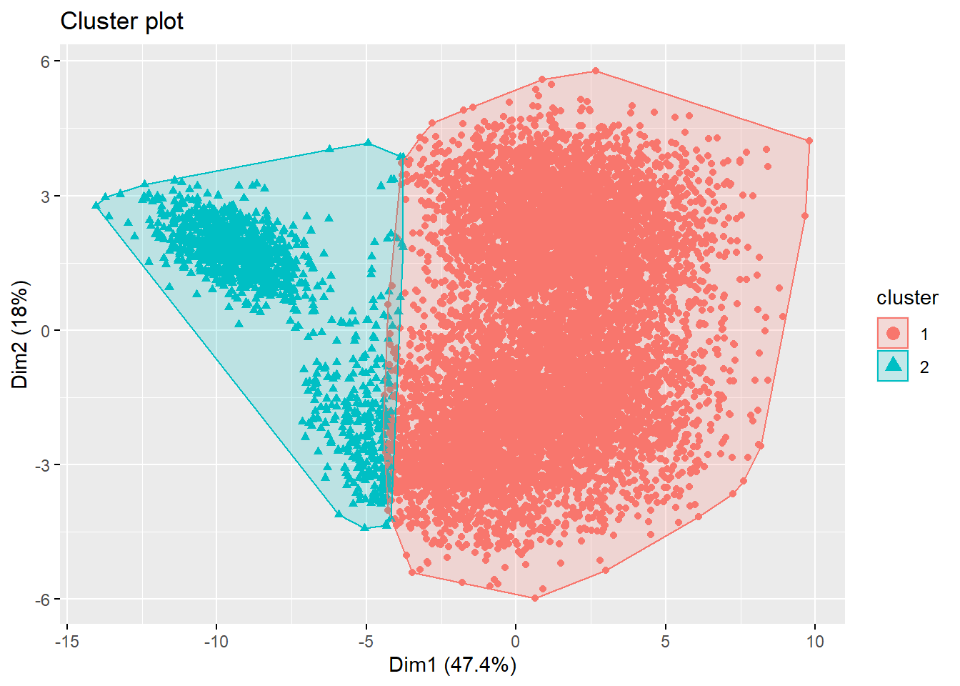 Looking at the plot, it seems as if both options yield suboptimal results. Therefore, always check your results, as an alternative solution might be required. We could try the spectral clustering approach, with the suggested number of clusters (i.e., 3). However, spectral clustring mostly produces high-quality clusterings on small data sets, and has limited applicability to large scale problems due to its computational complexity. If you don’t believe me: try running this line of code:
# spectral3 <- specc(x=football_sc, centers=3,
# iterations=200, kernel='rbfdot', kpar = list(sigma = 15))

# fviz_cluster(list(data = football_sc, cluster =
# kms[[1]]$cluster), geom = 'point', ellipse.type =
# 'convex' )
Some may have experienced issues due to limited working memory (Error: cannot allocate vector of size …). This can be countered by fitting your clusters on a more limited sample size as is done in the example below (with 1000 samples). Note that the determination of optimal number of clusters with the NbClust method was also based on a limited sample size.
# Lets rebuild our football cluster for kmeans Since we
# don't know the optimal number, let's make a loop and
# decide upon the aforementioned metrics Check cluster
# validity for multiple values of k
kms <- list()

smaller_sample <- football_sc[random, ]

for (k in 2:6) {
    kms[[k]] <- kmeans(x = smaller_sample, centers = k, nstart = 50)
}

kms[[1]] <- NULL

# Silhouette index (maximize)
ds <- dist(smaller_sample, method = "euclidean")
sapply(kms, function(km) summary(silhouette(km$cluster, ds))$avg.width)
## [1] 0.4363922 0.2315783 0.2269328 0.2138149
## [5] 0.1822053# Dunn index (maximize)
p_load(clValid)
sapply(kms, function(km) dunn(ds, km$cluster))## [1] 0.1286129 0.1227784 0.1430272 0.1506762
## [5] 0.1585677# Davies-Bouldin index (minimize)
p_load(clusterSim)
sapply(kms, function(km) index.DB(smaller_sample, km$cluster)$DB)## [1] 0.9631697 1.4681063 1.4323039 1.4379298
## [5] 1.6415087# Choose optimal number of clusters k using all cluster
# validation measures (24 measures)
p_load(NbClust)
nbc <- NbClust(data = smaller_sample, min.nc = 2, max.nc = 5,
method = "kmeans", index = "all")
## *** : The Hubert index is a graphical method of determining the number of clusters.
##                 In the plot of Hubert index, we seek a significant knee that corresponds to a
##                 significant increase of the value of the measure i.e the significant peak in Hubert
##                 index second differences plot.
## 
## *** : The D index is a graphical method of determining the number of clusters.
##                 In the plot of D index, we seek a significant knee (the significant peak in Dindex
##                 second differences plot) that corresponds to a significant increase of the value of
##                 the measure.
##
## *******************************************************************
## * Among all indices:
## * 8 proposed 2 as the best number of clusters
## * 11 proposed 3 as the best number of clusters
## * 2 proposed 4 as the best number of clusters
## * 3 proposed 5 as the best number of clusters
##
##                    ***** Conclusion *****
##
## * According to the majority rule, the best number of clusters is  3
##
##
## *******************************************************************
# If we determine our number clusters on our full dataset,
# We can directly deploy the detected algorithms from this
# model Plot
fviz_cluster(list(data = smaller_sample, cluster = nbc$Best.partition),
geom = "point", ellipse.type = "convex")