2 Preprocessing
This chapter will cover the concepts seen in Session 1 Preprocessing. Make sure that you go over the video and slides before going over this chapter.
Throughout the book and the exercises, we will be using data from a newpaper publishing company. A newspaper publishing company (NPC) has contacted you to address their increasing churn rates. This evolution has been jumpstarted by the rise of news-websites, and has continued at an accelerating rate due to the popularity of tablet computers and (social) news-aggregator applications. Hence the NPC requires a predictive retention (or churn) model in order to predict which customers will not renew their newspaper subscriptions. Before building a predictive model, a data scientist must always get some understanding of the data (e.g., plots and summary statistics) and solve several data quality issues. Also, before the data can be used in a predictive model several preprocessing steps have to be performed and features should be created.
The company has provided you two tables to start with:
Customers: contains socio-demographic data about the customers.
Subscription: contains information about the subscriptions of NPC’s customers.
Customers
| Variable | Description |
|---|---|
| CustomerID | Unique customer identifier |
| Gender | M = Male, F = Female, NA = Not Available |
| DoB | Date of Birth |
| District | Macro-geographical grouping: district 1-8 |
| ZIP | Meso-geographical grouping |
| StreeID | Micro-geographical grouping: street identifiers |
Subscriptions
| Variable | Description |
|---|---|
| SubscriptionID | Unique subscription identifier |
| CustomerID | Customer identifier |
| ProductID | Product identifier |
| Pattern | Denotes delivery days. The position in the string equals the days in the week. {1=delivery, 0=non-delivery} e.g., 1000000 = delivery only on Monday 1111110 = delivery on all days (except Sundays) |
| StartDate | Subscription start date |
| EndDate | Subscription end date |
| NbrNewspapers | Total number of copies including NbrStart as determined at the start of the subscription. |
| NbrStart | Maximum number of copies before payment is received. |
| RenewalDate | Date that renewal is processed. |
| PaymentType | BT = Bank transfer, DD = Direct debit |
| PaymentStatus | Paid and Not Paid |
| PaymentDate | Date of payment |
| FormulaID | Formula identifier |
| GrossFormulaPrice | GrossFormulaPrice = NetFormulaPrice + TotalDiscount |
| NetFormulaPrice | NetFormulaPrice = GrossFormulaPrice –TotalDiscount |
| NetNewspaperPrice | Price of a single newspaper |
| ProductDiscount | Discount based on the product |
| FormulaDiscount | Discount based on the formula |
| TotalDiscount | TotalDiscount = ProductDiscount + FormulaDiscount |
| TotalPrice | TotalPrice = NbrNewspapers * NetNewspaperPrice OR TotalPrice = NetFormulaPrice + TotalCredit |
| TotalCredit | The customer’s credit of previous transactions. Credit is negative, debit is positive. |
The goal will be to explore the data, solve possible quality issues and effectively prepare the data. The prepared basetable should contain the traditional RFM variables from the subscriptions table and some socio-demographics from the customers tables.
Before performing advanced preprocessing and feature engineering. Let’s first read in and explore the data.
2.1 Data understanding
Before we can read in the data, we should load the necessary packages. For data understanding and preparation, we will heavily use the tidyverse approach (check https://www.tidyverse.org/ for more information). The student should be able understand and code all of the given examples. If a student wants more explanation and practice in the tidyverse, they can follow the suggested Datacamp courses on Ufora.
if (!require("pacman")) install.packages("pacman")
require("pacman", character.only = TRUE, quietly = TRUE)
p_load(tidyverse)
2.1.1 Reading in the data
First and foremost, we must set the working directory and read the data from disk before. If your are working in a normal R script, you can do this with the setwd("Your working directory") command.
Since this books works in a notebook, we have to change the directory of our notebook. The notebook directory is by default the directory where your Rmd file is located. Since our data is located at another directory, we have to change the root.dir of knitr. Be aware that if you would use the setwd("Your working directory") command, you only change the working directory for that specific code chunk.
p_load(knitr)
knitr::opts_knit$set(root.dir = "C:\\Users\\matbogae\\OneDrive - UGent\\PPA22\\PredictiveAnalytics\\Book_2022\\data codeBook_2022")
getwd()
## [1] "C:/Users/matbogae/OneDrive - UGent/PPA22/PredictiveAnalytics/Book_2022"Subscriptions table
Let’s now read in the data.
# Since it is a text file with a ';' you can use the
# universal read.table command
subscriptions <- read.table(file = "subscriptions.txt", header = TRUE,
    sep = ";")

# However, we prefer the read_delim function of the
# tidyverse, and use ';' as delim
subscriptions <- read_delim(file = "subscriptions.txt", delim = ";",
    col_names = TRUE)
## Rows: 8252 Columns: 21## -- Column specification --------------------------
## Delimiter: ";"
## chr (7): Pattern, StartDate, EndDate, Renewal...
## dbl (14): SubscriptionID, CustomerID, ProductI...##
## i Use `spec()` to retrieve the full column specification for this data.
## i Specify the column types or set `show_col_types = FALSE` to quiet this message.# Let's take a glimpse at the structure of the data. We see
# that there are 8252 observations, and 21 variables along
# with the first couple of values of each variable
subscriptions %>%
glimpse()## Rows: 8,252
## Columns: 21
## $ SubscriptionID <dbl> 1000687, 1000823, 1001~
## $ CustomerID <dbl> 286997, 659050, 608896~
## $ ProductID <dbl> 8, 5, 3, 8, 8, 8, 8, 8~
## $ Pattern <chr> "1111110", "1111110", ~
## $ StartDate <chr> "13/02/2010", "30/01/2~
## $ EndDate <chr> "14/08/2010", "27/02/2~
## $ NbrNewspapers <dbl> 152, 25, 25, 25, 25, 3~
## $ NbrStart <dbl> 10, 10, 25, 25, 25, 10~
## $ RenewalDate <chr> "15/07/2010", "11/02/2~
## $ PaymentType <chr> "BT", "DD", "DD", "BT"~
## $ PaymentStatus <chr> "Paid", "Paid", "Paid"~
## $ PaymentDate <chr> "09/02/2010", "20/01/2~
## $ FormulaID <dbl> 8636, 9417, 5389, 4688~
## $ GrossFormulaPrice <dbl> 148.0, 27.0, 22.9, 22.~
## $ NetFormulaPrice <dbl> 148.0, 27.0, 22.9, 22.~
## $ NetNewspaperPrice <dbl> 0.973684, 1.080000, 0.~
## $ ProductDiscount <dbl> 0, 0, 0, 0, 0, 0, 0, 0~
## $ FormulaDiscount <dbl> 0, 0, 0, 0, 0, 0, 0, 0~
## $ TotalDiscount <dbl> 0, 0, 0, 0, 0, 0, 0, 0~
## $ TotalPrice <dbl> 148.0, 27.0, 22.9, 22.~
## $ TotalCredit <dbl> 0, 0, 0, 0, 0, 0, 0, 0~# One way to speed up the reading, is to specify the
# classes of the columns (col_types) upfront. For example,
# the Paymentstatus and PaymentType are characters, but it
# better to put them as factor. Sometimes read_delim might
# mix up the decimal separator, so it is good practice to
# specify it with the locale option
# see ?read_delim for more options
subscriptions <- read_delim(file = "subscriptions.txt", delim = ";",
col_names = TRUE, col_types = cols("c", "c", "c", "c", "c",
"c", "i", "i", "c", "f", "f", "c", "c", "n", "n", "n",
"n", "n", "n", "n", "n"), locale = locale(decimal_mark = "."))
# If we are reading in a table for the first time, and we
# don't know the classes, we can use the n_max parameter in
# read_delim
subscriptions <- read_delim(file = "subscriptions.txt", col_names = TRUE,
delim = ";", n_max = 5)## Rows: 5 Columns: 21## -- Column specification --------------------------
## Delimiter: ";"
## chr (6): StartDate, EndDate, RenewalDate, Pay...
## dbl (15): SubscriptionID, CustomerID, ProductI...##
## i Use `spec()` to retrieve the full column specification for this data.
## i Specify the column types or set `show_col_types = FALSE` to quiet this message.subscriptions <- read_delim(file = "subscriptions.txt", col_names = TRUE,
delim = ";", col_types = cols("c", "c", "c", "c", "c", "c",
"i", "i", "c", "f", "f", "c", "c", "n", "n", "n", "n",
"n", "n", "n", "n"))
# Another very fast option is to use the fread function of
# data.table, which is blazingly fast And does not really
# require you to set any other parameters, because
# everything is optimized! p_load(data.table) subscription
# <- fread('subscriptions.txt')Customers table
customers <- read_delim(file = "customers.txt", delim = ";",
    col_names = TRUE, col_types = cols("i", "f", "c", "f", "c",
        "c"))

# Let's have a glimpse as well
customers %>%
    glimpse()
## Rows: 1,389
## Columns: 6
## $ CustomerID <int> 106785, 910656, 913085, 65831~
## $ Gender <fct> M, F, M, M, M, , M, M, M, , F~
## $ DOB <chr> "09/11/1934", "16/06/1974", "~
## $ District <fct> 5, 5, 5, 1, 1, 5, 1, 5, 1, 5,~
## $ ZIP <chr> "3910", "3510", "3500", "2800~
## $ StreeID <chr> "46362", "37856", "37513", "2~2.1.2 Working with dates
As you might have noticed, when reading in the data, dates are read in as a character vector. The function as.Date() from the base package creates a Date object. Most systems store dates internally as the number of days (numeric vector) since some origin. When using as.Date or as_date on a numeric vector we need to set the origin. The origin on this system (and most systems) is “1970/01/01”.
# For more information look at the help function ?as.DateThe tidyverse alternative for dates is the lubridate package. For a nice overview of all the functionalities of lubridate, have a look at the cheatsheet: https://rawgit.com/rstudio/cheatsheets/master/lubridate.pdf.
p_load(lubridate)
# ?as_date
Let’s have a closer look how both packages handle dates.
# This is how you find out what the origin is:
Sys.Date() - as.integer(Sys.Date())
## [1] "1970-01-01"# This is Today's date:
Sys.Date()## [1] "2022-02-07"# Converting an integer requires an origin:
as.Date(10, origin = "1970/01/01")## [1] "1970-01-11"as_date(10, origin = "1970/01/01")## [1] "1970-01-11"# formats for base Date functions %d day as a number %a
# abbreviated weekday %A unabbreviated weekday %m month %b
# abbreviated month %B unabbreviated month %y 2-digit year
# %Y 4-digit year
# More information: help(strftime) help(ISOdatetime)
# Specifying a date format:
f <- "%d/%m/%Y"
# Subtraction of two dates as Date object using the format:
as.Date("02/01/1970", format = f) - as.Date("01/01/1970", format = f)## Time difference of 1 days# Lubridate does not work with this syntax but rather with
# dmy() = day month year
dmy("02/01/1970") - dmy("01/01/1970")## Time difference of 1 days# Subtraction of two dates as numeric objects:
as.numeric(as.Date("02/01/1970", format = f)) - as.numeric(as.Date("01/01/1970",
format = f))## [1] 1# OR
as.numeric(dmy("02/01/1970")) - as.numeric(dmy("01/01/1970"))## [1] 1# Adding zero days to the origin should be 0:
as.numeric(as.Date(0, origin = "1970/01/01"))## [1] 0# OR
as.numeric(as_date(0, origin = "1970/01/01"))## [1] 0Now let’s apply this knowledge, to our data sets.
# For the subscriptions table Let's just have a look at a
# data variable to know the format
subscriptions %>%
    pull(StartDate) %>%
    head()
## [1] "13/02/2010" "30/01/2010" "30/01/2010"
## [4] "13/02/2010" "16/01/2010" "14/02/2010"# Get the positions of the date variables
(vars <- which(names(subscriptions) %in% c("StartDate", "EndDate",
"PaymentDate", "RenewalDate")))## [1] 5 6 9 12# Transform to dates
subscriptions[, vars] <- subscriptions[, vars] %>%
map_df(., function(x) dmy(x))
# Check whether everything is okay You will notice that the
# desired variables have changed to 'date'
subscriptions %>%
glimpse()## Rows: 8,252
## Columns: 21
## $ SubscriptionID <chr> "1000687", "1000823", ~
## $ CustomerID <chr> "286997", "659050", "6~
## $ ProductID <chr> "8", "5", "3", "8", "8~
## $ Pattern <chr> "1111110", "1111110", ~
## $ StartDate <date> 2010-02-13, 2010-01-3~
## $ EndDate <date> 2010-08-14, 2010-02-2~
## $ NbrNewspapers <int> 152, 25, 25, 25, 25, 3~
## $ NbrStart <int> 10, 10, 25, 25, 25, 10~
## $ RenewalDate <date> 2010-07-15, 2010-02-1~
## $ PaymentType <fct> BT, DD, DD, BT, BT, BT~
## $ PaymentStatus <fct> Paid, Paid, Paid, Paid~
## $ PaymentDate <date> 2010-02-09, 2010-01-2~
## $ FormulaID <chr> "8636", "9417", "5389"~
## $ GrossFormulaPrice <dbl> 148.0, 27.0, 22.9, 22.~
## $ NetFormulaPrice <dbl> 148.0, 27.0, 22.9, 22.~
## $ NetNewspaperPrice <dbl> 0.973684, 1.080000, 0.~
## $ ProductDiscount <dbl> 0, 0, 0, 0, 0, 0, 0, 0~
## $ FormulaDiscount <dbl> 0, 0, 0, 0, 0, 0, 0, 0~
## $ TotalDiscount <dbl> 0, 0, 0, 0, 0, 0, 0, 0~
## $ TotalPrice <dbl> 148.0, 27.0, 22.9, 22.~
## $ TotalCredit <dbl> 0, 0, 0, 0, 0, 0, 0, 0~subscriptions %>%
pull(StartDate) %>%
head()## [1] "2010-02-13" "2010-01-30" "2010-01-30"
## [4] "2010-02-13" "2010-01-16" "2010-02-14"# For the customers table
customers$DOB <- dmy(customers$DOB)2.1.3 Data exploration
To get an understanding of the data, we will perform some statistical and visual data exploration.
Basic commands
# What are the dimensions of the data? The first number is
# the number of rows, the second number is the number of
# columns?
dim(subscriptions)
## [1] 8252 21nrow(subscriptions) #same as dim(subscriptions)[1]## [1] 8252ncol(subscriptions) #same as dim(subscriptions)[2]## [1] 21# Look at the structure of the object
# str(subscriptions,vec.len=0.5)
subscriptions %>%
glimpse()## Rows: 8,252
## Columns: 21
## $ SubscriptionID <chr> "1000687", "1000823", ~
## $ CustomerID <chr> "286997", "659050", "6~
## $ ProductID <chr> "8", "5", "3", "8", "8~
## $ Pattern <chr> "1111110", "1111110", ~
## $ StartDate <date> 2010-02-13, 2010-01-3~
## $ EndDate <date> 2010-08-14, 2010-02-2~
## $ NbrNewspapers <int> 152, 25, 25, 25, 25, 3~
## $ NbrStart <int> 10, 10, 25, 25, 25, 10~
## $ RenewalDate <date> 2010-07-15, 2010-02-1~
## $ PaymentType <fct> BT, DD, DD, BT, BT, BT~
## $ PaymentStatus <fct> Paid, Paid, Paid, Paid~
## $ PaymentDate <date> 2010-02-09, 2010-01-2~
## $ FormulaID <chr> "8636", "9417", "5389"~
## $ GrossFormulaPrice <dbl> 148.0, 27.0, 22.9, 22.~
## $ NetFormulaPrice <dbl> 148.0, 27.0, 22.9, 22.~
## $ NetNewspaperPrice <dbl> 0.973684, 1.080000, 0.~
## $ ProductDiscount <dbl> 0, 0, 0, 0, 0, 0, 0, 0~
## $ FormulaDiscount <dbl> 0, 0, 0, 0, 0, 0, 0, 0~
## $ TotalDiscount <dbl> 0, 0, 0, 0, 0, 0, 0, 0~
## $ TotalPrice <dbl> 148.0, 27.0, 22.9, 22.~
## $ TotalCredit <dbl> 0, 0, 0, 0, 0, 0, 0, 0~# Display the first couple of rows
head(subscriptions)## # A tibble: 6 x 21
## SubscriptionID CustomerID ProductID Pattern
## <chr> <chr> <chr> <chr>
## 1 1000687 286997 8 1111110
## 2 1000823 659050 5 1111110
## 3 1001004 608896 3 1111110
## 4 1001130 799769 8 1111110
## 5 1001564 451025 8 1111110
## 6 1002005 273071 8 1111110
## # ... with 17 more variables: StartDate <date>,
## # EndDate <date>, NbrNewspapers <int>,
## # NbrStart <int>, RenewalDate <date>,
## # PaymentType <fct>, PaymentStatus <fct>,
## # PaymentDate <date>, FormulaID <chr>,
## # GrossFormulaPrice <dbl>,
## # NetFormulaPrice <dbl>, ...# Display the last couple of rows
tail(subscriptions)## # A tibble: 6 x 21
## SubscriptionID CustomerID ProductID Pattern
## <chr> <chr> <chr> <chr>
## 1 999409 654047 7 1111110
## 2 999518 677422 6 1111110
## 3 999536 735141 3 0001000
## 4 999592 724712 2 1111110
## 5 999701 497901 8 1111110
## 6 999848 1115876 1 1111110
## # ... with 17 more variables: StartDate <date>,
## # EndDate <date>, NbrNewspapers <int>,
## # NbrStart <int>, RenewalDate <date>,
## # PaymentType <fct>, PaymentStatus <fct>,
## # PaymentDate <date>, FormulaID <chr>,
## # GrossFormulaPrice <dbl>,
## # NetFormulaPrice <dbl>, ...# How long is a vector? This is the same as
# nrow(subscriptions)
length(subscriptions$PaymentStatus)## [1] 8252# What are the column names?
colnames(subscriptions) #or names(subscriptions)## [1] "SubscriptionID" "CustomerID"
## [3] "ProductID" "Pattern"
## [5] "StartDate" "EndDate"
## [7] "NbrNewspapers" "NbrStart"
## [9] "RenewalDate" "PaymentType"
## [11] "PaymentStatus" "PaymentDate"
## [13] "FormulaID" "GrossFormulaPrice"
## [15] "NetFormulaPrice" "NetNewspaperPrice"
## [17] "ProductDiscount" "FormulaDiscount"
## [19] "TotalDiscount" "TotalPrice"
## [21] "TotalCredit"# Look at a random subset of the data.
subscriptions[sample(1:nrow(subscriptions), 5), ]## # A tibble: 5 x 21
## SubscriptionID CustomerID ProductID Pattern
## <chr> <chr> <chr> <chr>
## 1 532760 671127 4 1111110
## 2 940370 104207 8 1111110
## 3 984652 1006986 7 1111110
## 4 189782 216602 8 1111110
## 5 721117 599124 3 1111110
## # ... with 17 more variables: StartDate <date>,
## # EndDate <date>, NbrNewspapers <int>,
## # NbrStart <int>, RenewalDate <date>,
## # PaymentType <fct>, PaymentStatus <fct>,
## # PaymentDate <date>, FormulaID <chr>,
## # GrossFormulaPrice <dbl>,
## # NetFormulaPrice <dbl>, ...# Frequencies
table(subscriptions$PaymentStatus)##
## Paid Not Paid
## 7831 421Visual data exploration
One of the major strengths of R is the plots and the superb plotting package ggplot2. Whilst the goal of this book is not to provide a comprehensive overview of all the plotting abilites of base R and ggplot2, we will briefly discuss some of the more important commands.
Remember that the ggplot2 syntax always looks like this:
-Data : ggplot(data = , ...)
-Mapping (aesthetics): mapping = aes(x = , y = ), if you want to add grouping variables use the col and fill option.
-Geometric object (geom): geom_point() if no data our mapping argument are specified this object inherits the data and the aesthetics from the ggplot() function.
-Summary stats: stat_smooth(method = 'loess')
#Many functions are object-oriented: the same function
#reacts differently to different data types, this is called method dispatching
#The plot function in base R works like this, as well as the qplot function
#of ggplot2

plot(subscriptions$PaymentStatus)
plot(sort(subscriptions$TotalPrice))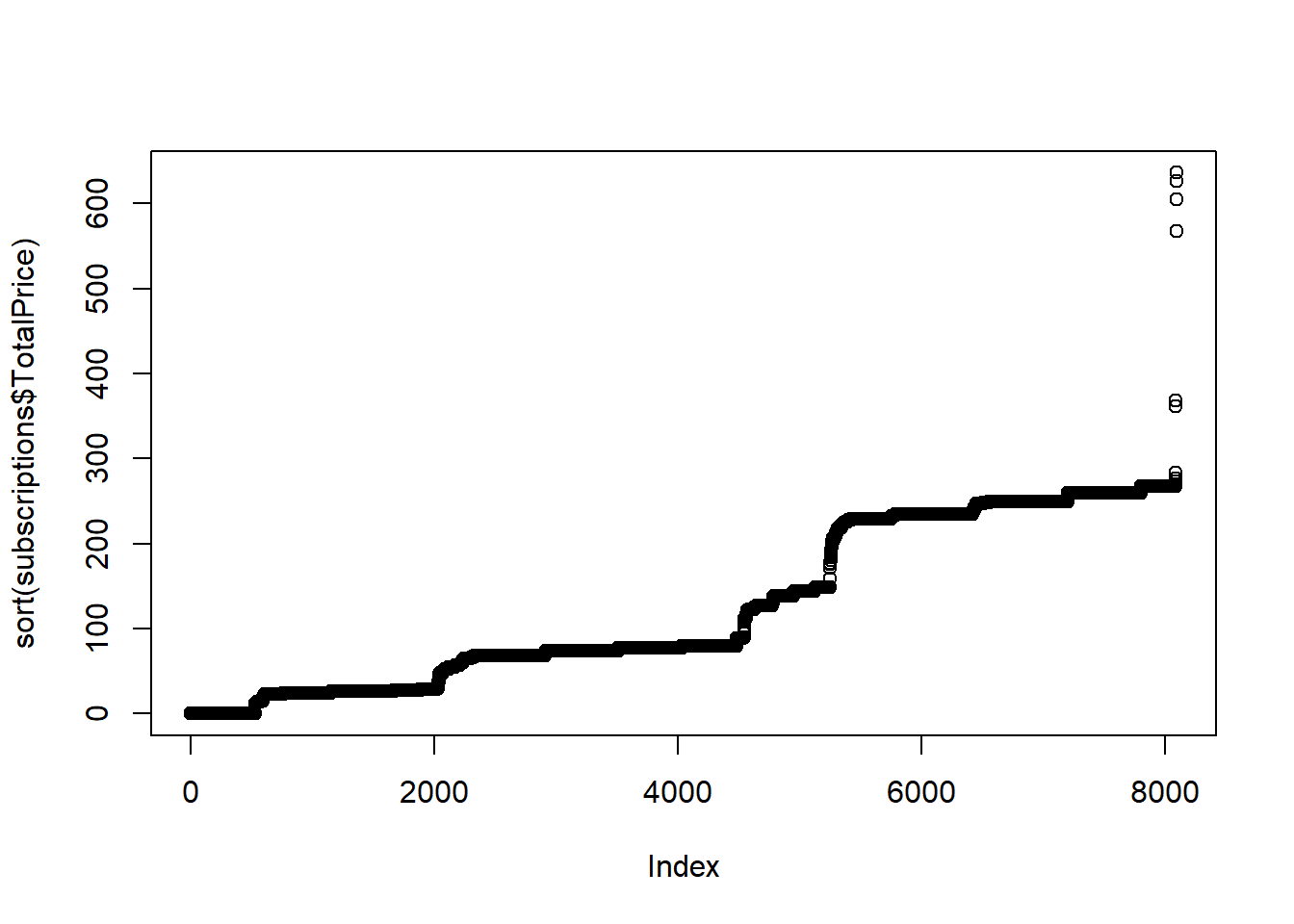
pairs(subscriptions[,17:21]) # a scatterplot matrix of variables in the data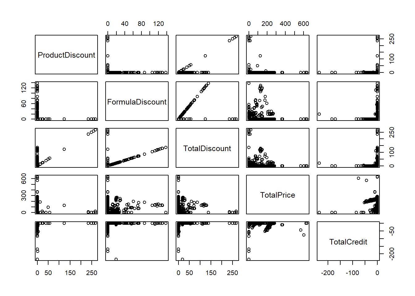
#Scatterplot
plot(subscriptions$NbrNewspapers,subscriptions$TotalPrice)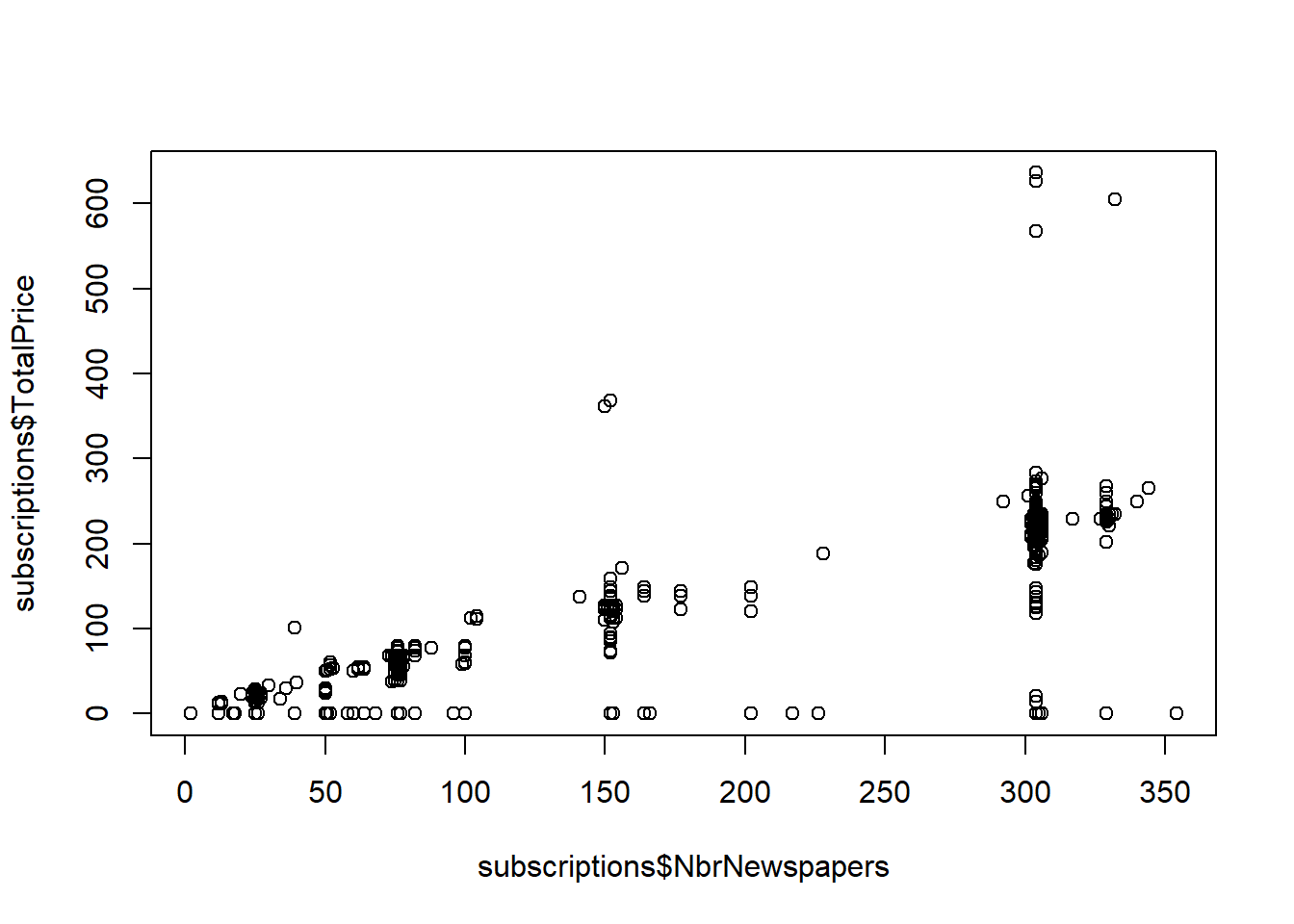
#Or with ggplot
subscriptions %>% ggplot(., aes(NbrNewspapers, TotalPrice)) + geom_point()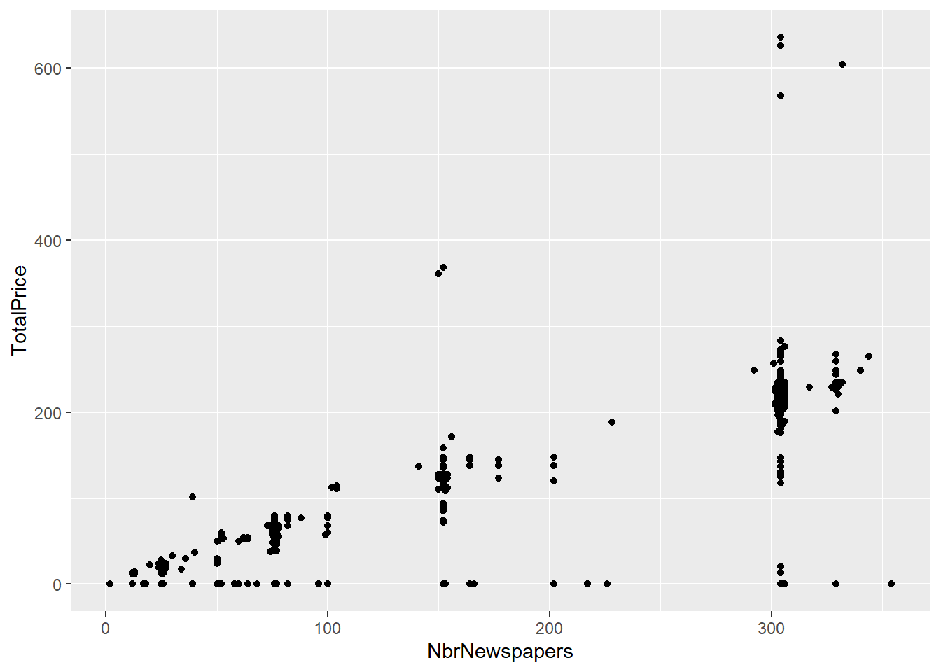
#Add a regression line
subscriptions %>% ggplot(., aes(NbrNewspapers, TotalPrice)) + geom_point() +
  stat_smooth(method = "lm")
## `geom_smooth()` using formula 'y ~ x'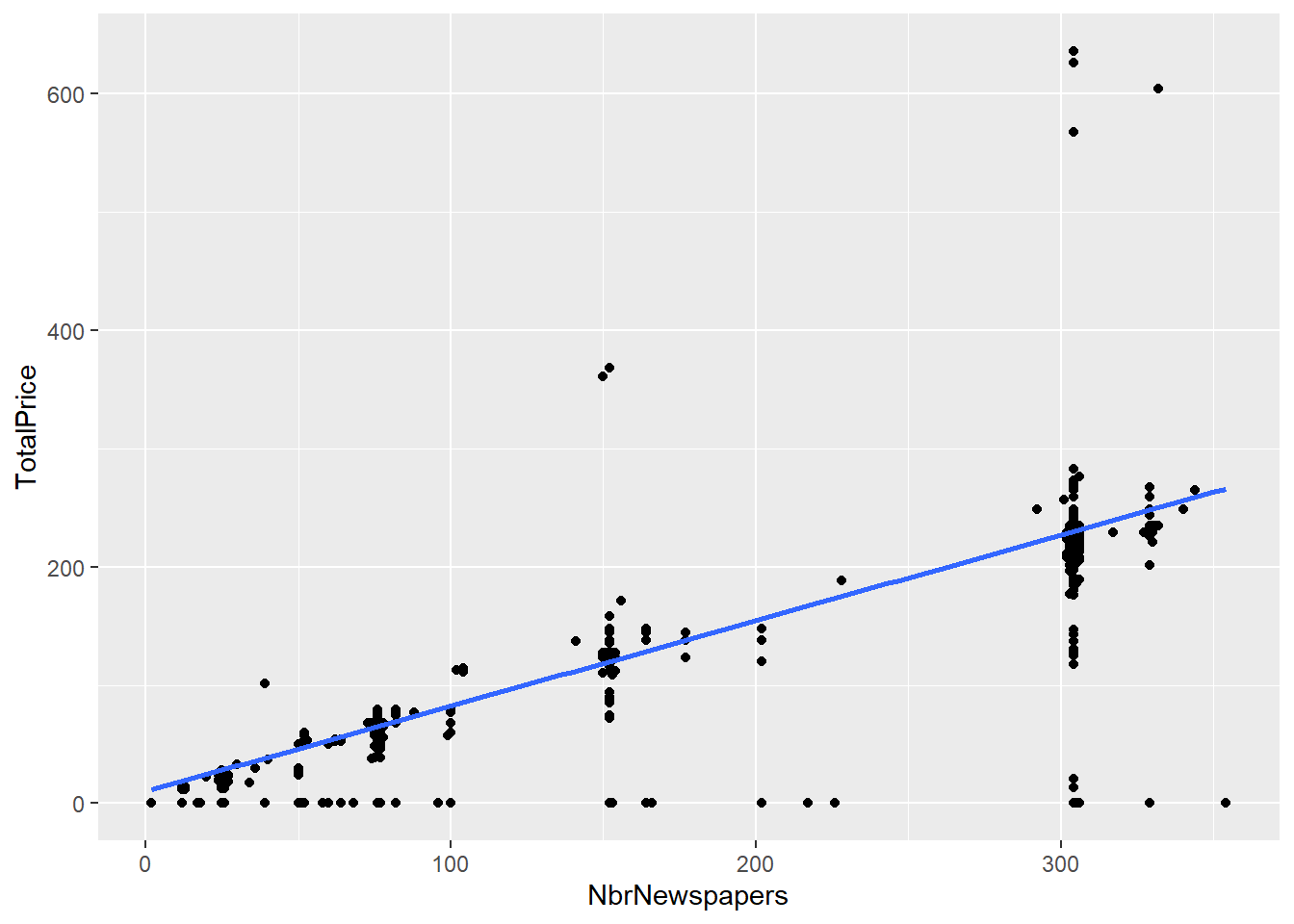
#Or a loess smoother
subscriptions %>% ggplot(., aes(NbrNewspapers, TotalPrice)) + geom_point() +
  stat_smooth(method = "loess")
## `geom_smooth()` using formula 'y ~ x'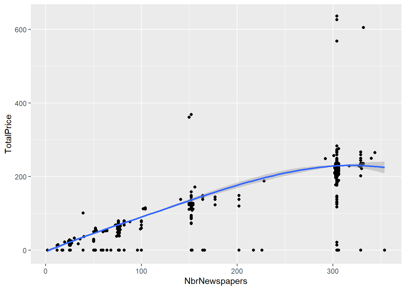
#You can even build a GAM with a cubic regression spline
subscriptions %>% ggplot(., aes(NbrNewspapers, TotalPrice)) + geom_point() +
  stat_smooth(method = "gam")
## `geom_smooth()` using formula 'y ~ s(x, bs = "cs")'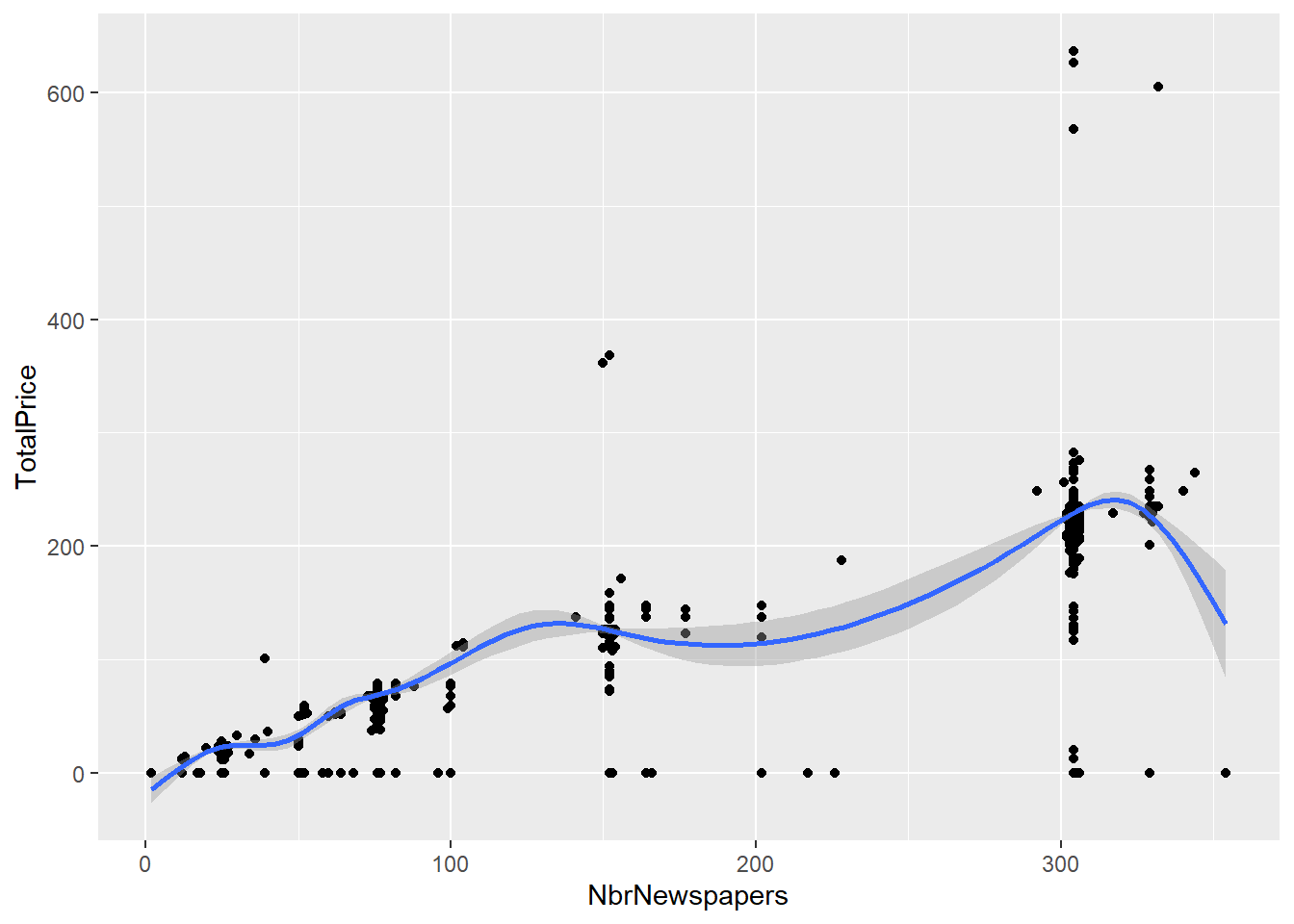
#A histogram of TotalPrice
hist(subscriptions$TotalPrice)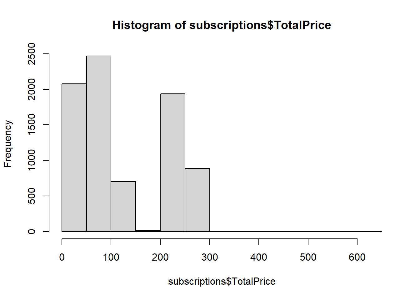
qplot(subscriptions$TotalPrice)## `stat_bin()` using `bins = 30`. Pick better
## value with `binwidth`.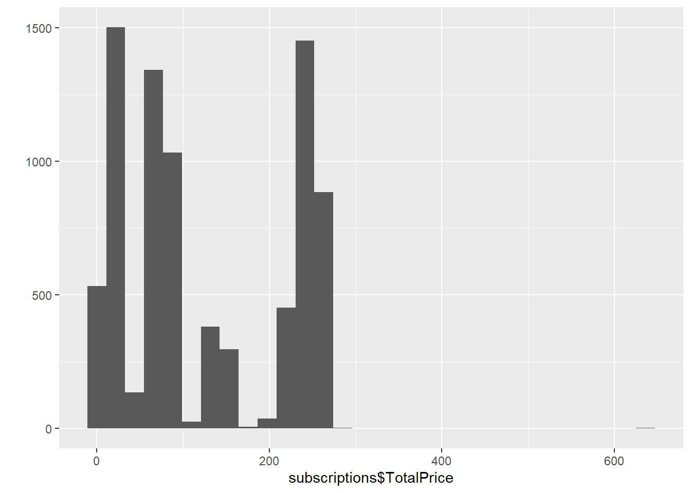
subscriptions %>% ggplot(., aes(TotalPrice)) + geom_histogram(binwidth = 10)
#A box plot of total price and payment type
subscriptions %>% ggplot(., aes(y = TotalPrice, fill = PaymentType)) +
  geom_boxplot()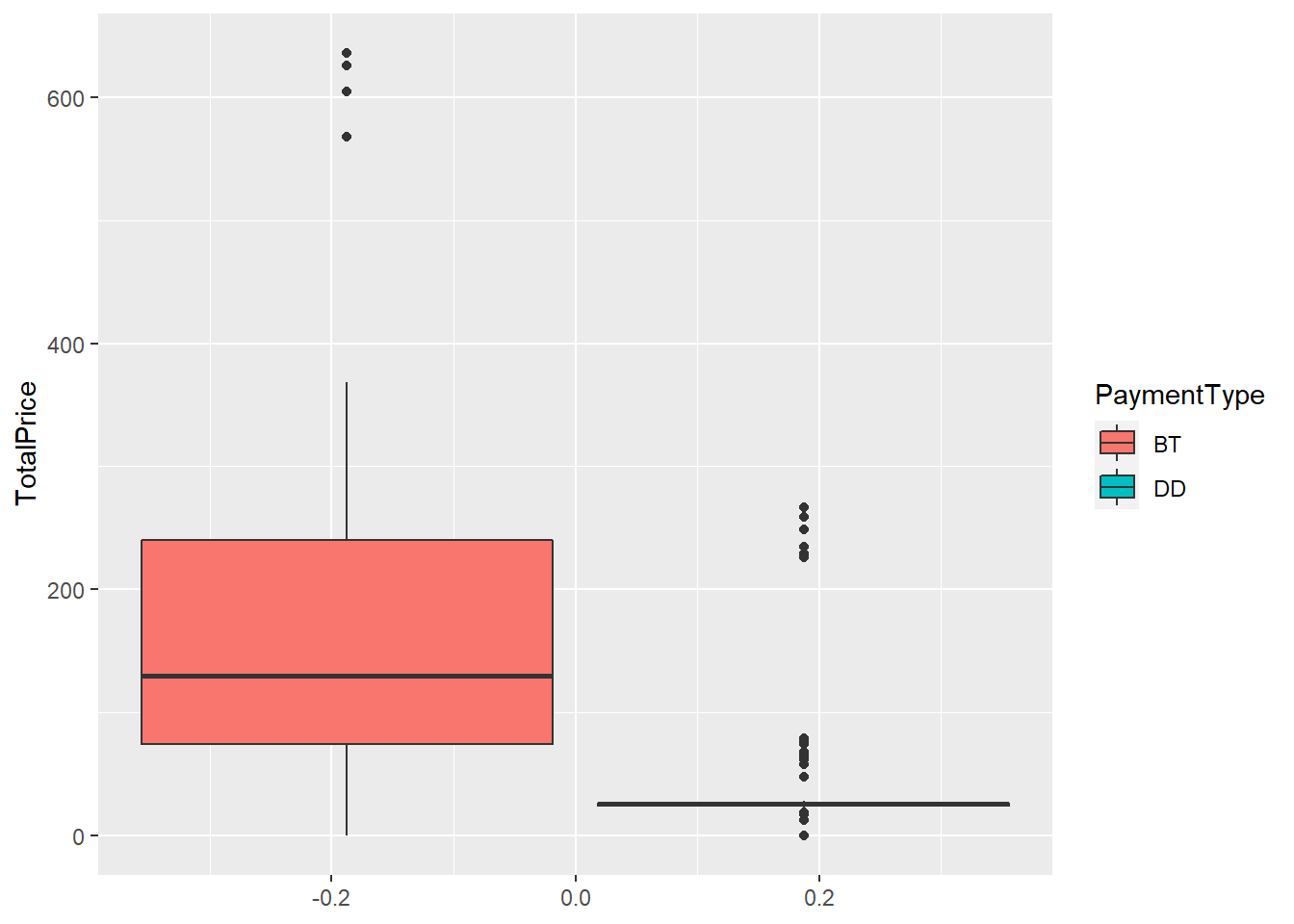
Statistical data exploration
#summarize a factor
summary(subscriptions$PaymentStatus)
## Paid Not Paid
## 7831 421#summarize a numeric variable
summary(subscriptions$TotalPrice)## Min. 1st Qu. Median Mean 3rd Qu. Max.
## 0.0 29.6 79.0 125.4 235.0 636.0
## NA's
## 161#Mean
mean(subscriptions$TotalPrice, na.rm=TRUE)## [1] 125.372#Variance
var(subscriptions$TotalPrice, na.rm=TRUE)## [1] 9047.803#Standard deviation
sd(subscriptions$TotalPrice, na.rm=TRUE)## [1] 95.11994#Which values are not missing in TotalPrice?
head(!is.na(subscriptions$TotalPrice))## [1] TRUE TRUE TRUE TRUE TRUE TRUE#Correlation between two variables
cor(subscriptions$TotalPrice[!is.na(subscriptions$TotalPrice)],
subscriptions$NbrNewspapers[!is.na(subscriptions$TotalPrice)])## [1] 0.8988953#Range of a variable
range(subscriptions$TotalPrice[!is.na(subscriptions$TotalPrice)])## [1] 0.00 635.96#Minimum
min(subscriptions$TotalPrice, na.rm=TRUE)## [1] 0#Maximum
max(subscriptions$TotalPrice, na.rm=TRUE)## [1] 635.96#Is this a numeric vector?
is.numeric(subscriptions$TotalPrice)## [1] TRUEis.numeric(subscriptions$CustomerID)## [1] FALSE#It is much easier to plot all the statistic in one table for all variables
#The summary function can be messy though ...
summary(subscriptions)## SubscriptionID CustomerID
## Length:8252 Length:8252
## Class :character Class :character
## Mode :character Mode :character
##
##
##
##
## ProductID Pattern
## Length:8252 Length:8252
## Class :character Class :character
## Mode :character Mode :character
##
##
##
##
## StartDate EndDate
## Min. :2006-01-02 Min. :2007-01-02
## 1st Qu.:2007-09-30 1st Qu.:2008-03-08
## Median :2008-10-01 Median :2009-03-17
## Mean :2008-09-09 Mean :2009-03-11
## 3rd Qu.:2009-09-11 3rd Qu.:2010-02-18
## Max. :2011-02-24 Max. :2011-03-02
##
## NbrNewspapers NbrStart
## Min. : 2.0 Min. : 0
## 1st Qu.: 76.0 1st Qu.:10
## Median : 77.0 Median :10
## Mean :159.8 Mean :15
## 3rd Qu.:304.0 3rd Qu.:25
## Max. :354.0 Max. :30
## NA's :21
## RenewalDate PaymentType PaymentStatus
## Min. :2007-09-26 BT:6743 Paid :7831
## 1st Qu.:2008-09-01 DD:1509 Not Paid: 421
## Median :2009-06-01
## Mean :2009-06-08
## 3rd Qu.:2010-03-22
## Max. :2011-02-02
## NA's :2020
## PaymentDate FormulaID
## Min. :2005-12-14 Length:8252
## 1st Qu.:2007-08-30 Class :character
## Median :2008-09-15 Mode :character
## Mean :2008-08-17
## 3rd Qu.:2009-08-14
## Max. :2011-01-27
## NA's :421
## GrossFormulaPrice NetFormulaPrice
## Min. : 0.1697 Min. : 0.0
## 1st Qu.: 68.0000 1st Qu.: 68.0
## Median : 79.0000 Median : 79.0
## Mean :135.8778 Mean :133.3
## 3rd Qu.:235.0000 3rd Qu.:235.0
## Max. :310.9143 Max. :276.0
## NA's :161 NA's :161
## NetNewspaperPrice ProductDiscount
## Min. :0.0000 Min. : 0.000
## 1st Qu.:0.8092 1st Qu.: 0.000
## Median :0.8783 Median : 0.000
## Mean :0.8562 Mean : 2.459
## 3rd Qu.:0.9737 3rd Qu.: 0.000
## Max. :1.1200 Max. :267.000
## NA's :161 NA's :161
## FormulaDiscount TotalDiscount TotalPrice
## Min. : 0.000 Min. : 0 Min. : 0.0
## 1st Qu.: 0.000 1st Qu.: 0 1st Qu.: 29.6
## Median : 0.000 Median : 0 Median : 79.0
## Mean : 2.541 Mean : 5 Mean :125.4
## 3rd Qu.: 0.000 3rd Qu.: 0 3rd Qu.:235.0
## Max. :138.000 Max. :267 Max. :636.0
## NA's :161 NA's :161 NA's :161
## TotalCredit
## Min. :-235.0001
## 1st Qu.: 0.0000
## Median : 0.0000
## Mean : -0.5294
## 3rd Qu.: 0.0000
## Max. : 0.0000
## NA's :161#the psych package contains a nice describe function
p_load(psych)
psych::describe(subscriptions)## vars n mean sd
## SubscriptionID* 1 8252 4126.50 2382.29
## CustomerID* 2 8252 753.91 367.79
## ProductID* 3 8252 6.25 2.32
## Pattern* 4 8252 10.89 0.99
## StartDate 5 8252 NaN NA
## EndDate 6 8252 NaN NA
## NbrNewspapers 7 8252 159.82 117.97
## NbrStart 8 8231 15.00 7.29
## RenewalDate 9 6232 NaN NA
## PaymentType* 10 8252 1.18 0.39
## PaymentStatus* 11 8252 1.05 0.22
## PaymentDate 12 7831 NaN NA
## FormulaID* 13 8252 475.12 135.58
## GrossFormulaPrice 14 8091 135.88 92.60
## NetFormulaPrice 15 8091 133.34 93.25
## NetNewspaperPrice 16 8091 0.86 0.20
## ProductDiscount 17 8091 2.46 24.60
## FormulaDiscount 18 8091 2.54 10.73
## TotalDiscount 19 8091 5.00 26.60
## TotalPrice 20 8091 125.37 95.12
## TotalCredit 21 8091 -0.53 5.01
## median trimmed mad min
## SubscriptionID* 4126.50 4126.50 3058.60 1.00
## CustomerID* 773.00 760.04 440.33 1.00
## ProductID* 8.00 6.63 0.00 1.00
## Pattern* 11.00 11.00 0.00 1.00
## StartDate NA NaN NA Inf
## EndDate NA NaN NA Inf
## NbrNewspapers 77.00 158.51 78.58 2.00
## NbrStart 10.00 14.69 0.00 0.00
## RenewalDate NA NaN NA Inf
## PaymentType* 1.00 1.10 0.00 1.00
## PaymentStatus* 1.00 1.00 0.00 1.00
## PaymentDate NA NaN NA Inf
## FormulaID* 517.00 501.86 47.44 1.00
## GrossFormulaPrice 79.00 134.26 82.14 0.17
## NetFormulaPrice 79.00 131.66 82.14 0.00
## NetNewspaperPrice 0.88 0.89 0.14 0.00
## ProductDiscount 0.00 0.00 0.00 0.00
## FormulaDiscount 0.00 0.00 0.00 0.00
## TotalDiscount 0.00 0.08 0.00 0.00
## TotalPrice 79.00 122.84 83.17 0.00
## TotalCredit 0.00 0.00 0.00 -235.00
## max range skew kurtosis
## SubscriptionID* 8252.00 8251.00 0.00 -1.20
## CustomerID* 1389.00 1388.00 -0.12 -1.00
## ProductID* 8.00 7.00 -1.06 -0.28
## Pattern* 11.00 10.00 -9.43 87.99
## StartDate -Inf -Inf NA NA
## EndDate -Inf -Inf NA NA
## NbrNewspapers 354.00 352.00 0.29 -1.70
## NbrStart 30.00 30.00 0.46 -1.28
## RenewalDate -Inf -Inf NA NA
## PaymentType* 2.00 1.00 1.64 0.69
## PaymentStatus* 2.00 1.00 4.08 14.65
## PaymentDate -Inf -Inf NA NA
## FormulaID* 621.00 620.00 -1.72 2.15
## GrossFormulaPrice 310.91 310.74 0.24 -1.64
## NetFormulaPrice 276.00 276.00 0.25 -1.62
## NetNewspaperPrice 1.12 1.12 -2.57 8.46
## ProductDiscount 267.00 267.00 10.07 99.78
## FormulaDiscount 138.00 138.00 7.08 64.03
## TotalDiscount 267.00 267.00 8.14 70.76
## TotalPrice 635.96 635.96 0.37 -1.23
## TotalCredit 0.00 235.00 -26.81 1008.08
## se
## SubscriptionID* 26.22
## CustomerID* 4.05
## ProductID* 0.03
## Pattern* 0.01
## StartDate NA
## EndDate NA
## NbrNewspapers 1.30
## NbrStart 0.08
## RenewalDate NA
## PaymentType* 0.00
## PaymentStatus* 0.00
## PaymentDate NA
## FormulaID* 1.49
## GrossFormulaPrice 1.03
## NetFormulaPrice 1.04
## NetNewspaperPrice 0.00
## ProductDiscount 0.27
## FormulaDiscount 0.12
## TotalDiscount 0.30
## TotalPrice 1.06
## TotalCredit 0.062.1.4 Data quality
As mentioned in the slides, the most common data quality issues are:
- multicollinearity,
- missings values
- and outliers.
We will show in this section how to detect and hndle these issues.
2.1.4.1 Multicollinearity
Some basic correlation checking functions from base R:
# To check correlation, you must only focus on numeric
# variables
num <- subscriptions %>%
    select_if(is.numeric)

# The cor function is the basic function, use =
# 'complete.obs' This makes sure that NAs are removes The
# pearson correlation is used by default
cor(num, use = "complete.obs")
## NbrNewspapers NbrStart
## NbrNewspapers 1.000000000 -0.005760365
## NbrStart -0.005760365 1.000000000
## GrossFormulaPrice 0.993094452 -0.047692429
## NetFormulaPrice 0.987601066 -0.066964648
## NetNewspaperPrice -0.263394477 -0.089530891
## ProductDiscount 0.118920801 0.002573026
## FormulaDiscount -0.013726229 0.170440557
## TotalDiscount 0.104439967 0.071086115
## TotalPrice 0.898755683 -0.047748444
## TotalCredit -0.076992126 -0.062646229
## GrossFormulaPrice
## NbrNewspapers 0.993094452
## NbrStart -0.047692429
## GrossFormulaPrice 1.000000000
## NetFormulaPrice 0.993357985
## NetNewspaperPrice -0.239253882
## ProductDiscount 0.123407907
## FormulaDiscount -0.004171282
## TotalDiscount 0.112441179
## TotalPrice 0.894965233
## TotalCredit -0.070708252
## NetFormulaPrice
## NbrNewspapers 0.98760107
## NbrStart -0.06696465
## GrossFormulaPrice 0.99335798
## NetFormulaPrice 1.00000000
## NetNewspaperPrice -0.19170938
## ProductDiscount 0.12525766
## FormulaDiscount -0.11920740
## TotalDiscount 0.06777928
## TotalPrice 0.90130644
## TotalCredit -0.07160146
## NetNewspaperPrice
## NbrNewspapers -0.26339448
## NbrStart -0.08953089
## GrossFormulaPrice -0.23925388
## NetFormulaPrice -0.19170938
## NetNewspaperPrice 1.00000000
## ProductDiscount -0.42322276
## FormulaDiscount -0.39838536
## TotalDiscount -0.55197344
## TotalPrice -0.07438657
## TotalCredit 0.10630468
## ProductDiscount FormulaDiscount
## NbrNewspapers 0.118920801 -0.013726229
## NbrStart 0.002573026 0.170440557
## GrossFormulaPrice 0.123407907 -0.004171282
## NetFormulaPrice 0.125257660 -0.119207403
## NetNewspaperPrice -0.423222763 -0.398385356
## ProductDiscount 1.000000000 -0.023713925
## FormulaDiscount -0.023713925 1.000000000
## TotalDiscount 0.915200448 0.381182609
## TotalPrice -0.130254808 -0.110503163
## TotalCredit 0.010150644 0.012139029
## TotalDiscount TotalPrice
## NbrNewspapers 0.10443997 0.89875568
## NbrStart 0.07108612 -0.04774844
## GrossFormulaPrice 0.11244118 0.89496523
## NetFormulaPrice 0.06777928 0.90130644
## NetNewspaperPrice -0.55197344 -0.07438657
## ProductDiscount 0.91520045 -0.13025481
## FormulaDiscount 0.38118261 -0.11050316
## TotalDiscount 1.00000000 -0.16499960
## TotalPrice -0.16499960 1.00000000
## TotalCredit 0.01428030 -0.03404007
## TotalCredit
## NbrNewspapers -0.07699213
## NbrStart -0.06264623
## GrossFormulaPrice -0.07070825
## NetFormulaPrice -0.07160146
## NetNewspaperPrice 0.10630468
## ProductDiscount 0.01015064
## FormulaDiscount 0.01213903
## TotalDiscount 0.01428030
## TotalPrice -0.03404007
## TotalCredit 1.00000000# To make this less messy, you can round the number
round(cor(num, use = "complete.obs"), 2)## NbrNewspapers NbrStart
## NbrNewspapers 1.00 -0.01
## NbrStart -0.01 1.00
## GrossFormulaPrice 0.99 -0.05
## NetFormulaPrice 0.99 -0.07
## NetNewspaperPrice -0.26 -0.09
## ProductDiscount 0.12 0.00
## FormulaDiscount -0.01 0.17
## TotalDiscount 0.10 0.07
## TotalPrice 0.90 -0.05
## TotalCredit -0.08 -0.06
## GrossFormulaPrice
## NbrNewspapers 0.99
## NbrStart -0.05
## GrossFormulaPrice 1.00
## NetFormulaPrice 0.99
## NetNewspaperPrice -0.24
## ProductDiscount 0.12
## FormulaDiscount 0.00
## TotalDiscount 0.11
## TotalPrice 0.89
## TotalCredit -0.07
## NetFormulaPrice
## NbrNewspapers 0.99
## NbrStart -0.07
## GrossFormulaPrice 0.99
## NetFormulaPrice 1.00
## NetNewspaperPrice -0.19
## ProductDiscount 0.13
## FormulaDiscount -0.12
## TotalDiscount 0.07
## TotalPrice 0.90
## TotalCredit -0.07
## NetNewspaperPrice
## NbrNewspapers -0.26
## NbrStart -0.09
## GrossFormulaPrice -0.24
## NetFormulaPrice -0.19
## NetNewspaperPrice 1.00
## ProductDiscount -0.42
## FormulaDiscount -0.40
## TotalDiscount -0.55
## TotalPrice -0.07
## TotalCredit 0.11
## ProductDiscount FormulaDiscount
## NbrNewspapers 0.12 -0.01
## NbrStart 0.00 0.17
## GrossFormulaPrice 0.12 0.00
## NetFormulaPrice 0.13 -0.12
## NetNewspaperPrice -0.42 -0.40
## ProductDiscount 1.00 -0.02
## FormulaDiscount -0.02 1.00
## TotalDiscount 0.92 0.38
## TotalPrice -0.13 -0.11
## TotalCredit 0.01 0.01
## TotalDiscount TotalPrice
## NbrNewspapers 0.10 0.90
## NbrStart 0.07 -0.05
## GrossFormulaPrice 0.11 0.89
## NetFormulaPrice 0.07 0.90
## NetNewspaperPrice -0.55 -0.07
## ProductDiscount 0.92 -0.13
## FormulaDiscount 0.38 -0.11
## TotalDiscount 1.00 -0.16
## TotalPrice -0.16 1.00
## TotalCredit 0.01 -0.03
## TotalCredit
## NbrNewspapers -0.08
## NbrStart -0.06
## GrossFormulaPrice -0.07
## NetFormulaPrice -0.07
## NetNewspaperPrice 0.11
## ProductDiscount 0.01
## FormulaDiscount 0.01
## TotalDiscount 0.01
## TotalPrice -0.03
## TotalCredit 1.00Often researchers make correlation plots to get a nice and quik overview of the correlations between variables. The corrplot package makes nice correlation plot (see: https://cran.r-project.org/web/packages/corrplot/vignettes/corrplot-intro.html).
Another good package in R to perform correlation analysis is the correlation package. This package has tons of options to perform correlation analysis (also with binary vars) and by default a correlation test is performed.
There are also other packages available to create correlation plots, for example
-http://www.sthda.com/english/wiki/ggcorrplot-visualization-of-a-correlation-matrix-using-ggplot2
-https://github.com/tidymodels/corrr
We will only focus on the former two packages.
#A correlation plot of corrplot
p_load(corrplot)
p_load(see)

corr <- cor(num, use = 'complete.obs')
corrplot(corr, method = "circle")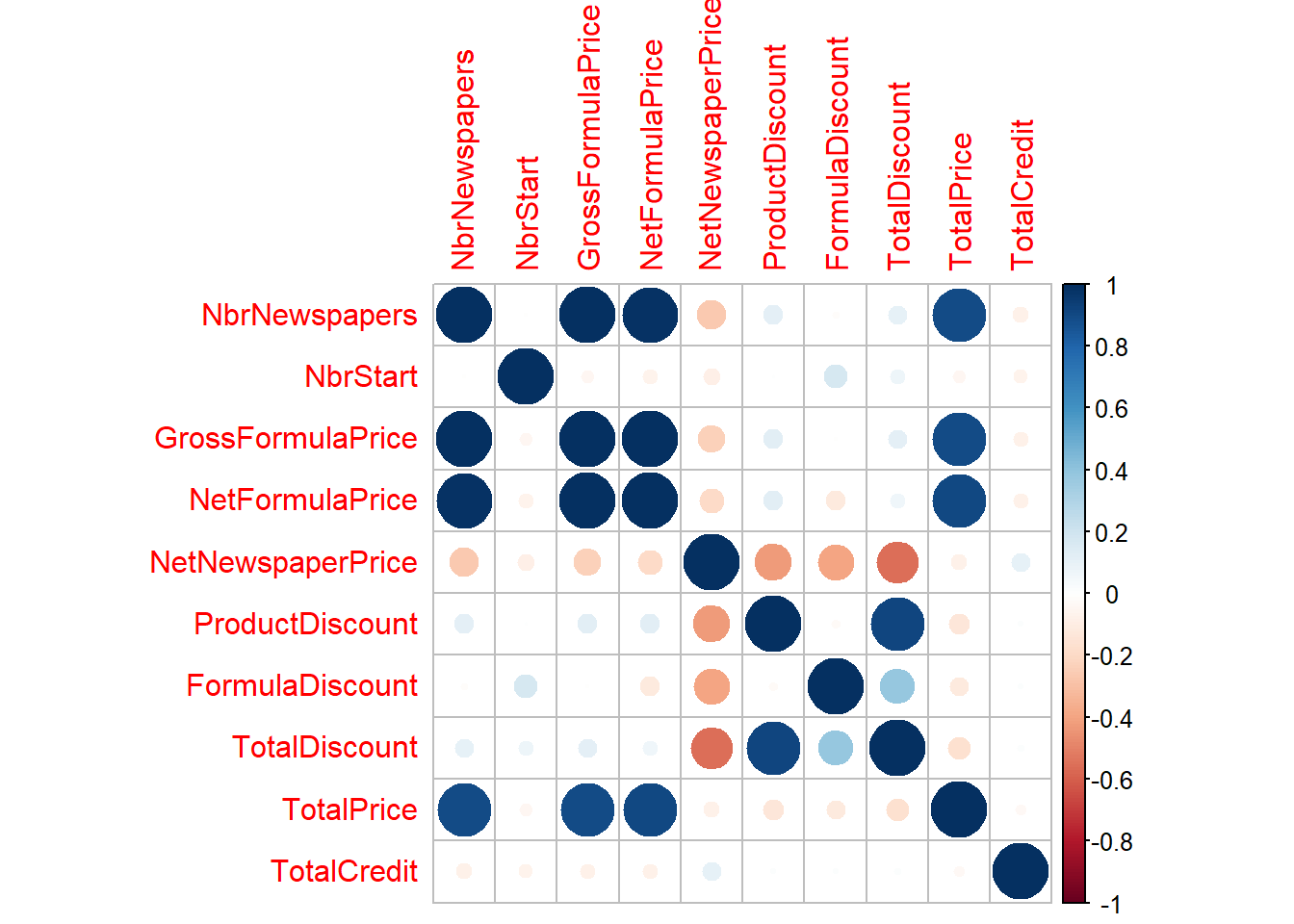
#The correlation package
p_load(correlation)

#The output is by default in the long format
correlation::correlation(subscriptions)
## # Correlation Matrix (pearson-method)
##
## Parameter1 | Parameter2 | r | 95% CI | t | df | p
## ----------------------------------------------------------------------------------------------
## NbrNewspapers | NbrStart | -9.32e-03 | [-0.03, 0.01] | -0.85 | 8229 | > .999
## NbrNewspapers | GrossFormulaPrice | 0.99 | [ 0.99, 0.99] | 761.50 | 8089 | < .001***
## NbrNewspapers | NetFormulaPrice | 0.99 | [ 0.99, 0.99] | 565.89 | 8089 | < .001***
## NbrNewspapers | NetNewspaperPrice | -0.26 | [-0.28, -0.24] | -24.60 | 8089 | < .001***
## NbrNewspapers | ProductDiscount | 0.12 | [ 0.10, 0.14] | 10.76 | 8089 | < .001***
## NbrNewspapers | FormulaDiscount | -0.01 | [-0.03, 0.01] | -1.18 | 8089 | > .999
## NbrNewspapers | TotalDiscount | 0.10 | [ 0.08, 0.13] | 9.46 | 8089 | < .001***
## NbrNewspapers | TotalPrice | 0.90 | [ 0.89, 0.90] | 184.51 | 8089 | < .001***
## NbrNewspapers | TotalCredit | -0.08 | [-0.10, -0.06] | -6.95 | 8089 | < .001***
## NbrStart | GrossFormulaPrice | -0.05 | [-0.07, -0.03] | -4.29 | 8070 | < .001***
## NbrStart | NetFormulaPrice | -0.07 | [-0.09, -0.05] | -6.03 | 8070 | < .001***
## NbrStart | NetNewspaperPrice | -0.09 | [-0.11, -0.07] | -8.08 | 8070 | < .001***
## NbrStart | ProductDiscount | 2.57e-03 | [-0.02, 0.02] | 0.23 | 8070 | > .999
## NbrStart | FormulaDiscount | 0.17 | [ 0.15, 0.19] | 15.54 | 8070 | < .001***
## NbrStart | TotalDiscount | 0.07 | [ 0.05, 0.09] | 6.40 | 8070 | < .001***
## NbrStart | TotalPrice | -0.05 | [-0.07, -0.03] | -4.29 | 8070 | < .001***
## NbrStart | TotalCredit | -0.06 | [-0.08, -0.04] | -5.64 | 8070 | < .001***
## GrossFormulaPrice | NetFormulaPrice | 0.99 | [ 0.99, 0.99] | 776.83 | 8089 | < .001***
## GrossFormulaPrice | NetNewspaperPrice | -0.24 | [-0.26, -0.22] | -22.20 | 8089 | < .001***
## GrossFormulaPrice | ProductDiscount | 0.12 | [ 0.10, 0.14] | 11.17 | 8089 | < .001***
## GrossFormulaPrice | FormulaDiscount | -3.59e-03 | [-0.03, 0.02] | -0.32 | 8089 | > .999
## GrossFormulaPrice | TotalDiscount | 0.11 | [ 0.09, 0.13] | 10.19 | 8089 | < .001***
## GrossFormulaPrice | TotalPrice | 0.90 | [ 0.89, 0.90] | 180.57 | 8089 | < .001***
## GrossFormulaPrice | TotalCredit | -0.07 | [-0.09, -0.05] | -6.38 | 8089 | < .001***
## NetFormulaPrice | NetNewspaperPrice | -0.19 | [-0.21, -0.17] | -17.61 | 8089 | < .001***
## NetFormulaPrice | ProductDiscount | 0.13 | [ 0.10, 0.15] | 11.35 | 8089 | < .001***
## NetFormulaPrice | FormulaDiscount | -0.12 | [-0.14, -0.10] | -10.74 | 8089 | < .001***
## NetFormulaPrice | TotalDiscount | 0.07 | [ 0.05, 0.09] | 6.12 | 8089 | < .001***
## NetFormulaPrice | TotalPrice | 0.90 | [ 0.90, 0.91] | 187.27 | 8089 | < .001***
## NetFormulaPrice | TotalCredit | -0.07 | [-0.09, -0.05] | -6.46 | 8089 | < .001***
## NetNewspaperPrice | ProductDiscount | -0.42 | [-0.44, -0.41] | -42.00 | 8089 | < .001***
## NetNewspaperPrice | FormulaDiscount | -0.40 | [-0.42, -0.38] | -39.07 | 8089 | < .001***
## NetNewspaperPrice | TotalDiscount | -0.55 | [-0.57, -0.54] | -59.53 | 8089 | < .001***
## NetNewspaperPrice | TotalPrice | -0.07 | [-0.10, -0.05] | -6.76 | 8089 | < .001***
## NetNewspaperPrice | TotalCredit | 0.11 | [ 0.08, 0.13] | 9.63 | 8089 | < .001***
## ProductDiscount | FormulaDiscount | -0.02 | [-0.05, 0.00] | -2.13 | 8089 | 0.265
## ProductDiscount | TotalDiscount | 0.92 | [ 0.91, 0.92] | 204.18 | 8089 | < .001***
## ProductDiscount | TotalPrice | -0.13 | [-0.15, -0.11] | -11.80 | 8089 | < .001***
## ProductDiscount | TotalCredit | 0.01 | [-0.01, 0.03] | 0.91 | 8089 | > .999
## FormulaDiscount | TotalDiscount | 0.38 | [ 0.36, 0.40] | 37.10 | 8089 | < .001***
## FormulaDiscount | TotalPrice | -0.11 | [-0.13, -0.09] | -9.94 | 8089 | < .001***
## FormulaDiscount | TotalCredit | 0.01 | [-0.01, 0.03] | 1.06 | 8089 | > .999
## TotalDiscount | TotalPrice | -0.16 | [-0.19, -0.14] | -15.01 | 8089 | < .001***
## TotalDiscount | TotalCredit | 0.01 | [-0.01, 0.04] | 1.27 | 8089 | > .999
## TotalPrice | TotalCredit | -0.03 | [-0.06, -0.01] | -3.07 | 8089 | 0.019*
##
## p-value adjustment method: Holm (1979)
## Observations: 8072-8231#This package also has a correlation plot
#although the options and layout in corrplot are nicer...
correlation::correlation(subscriptions) %>% summary(redundant = TRUE) %>%
plot()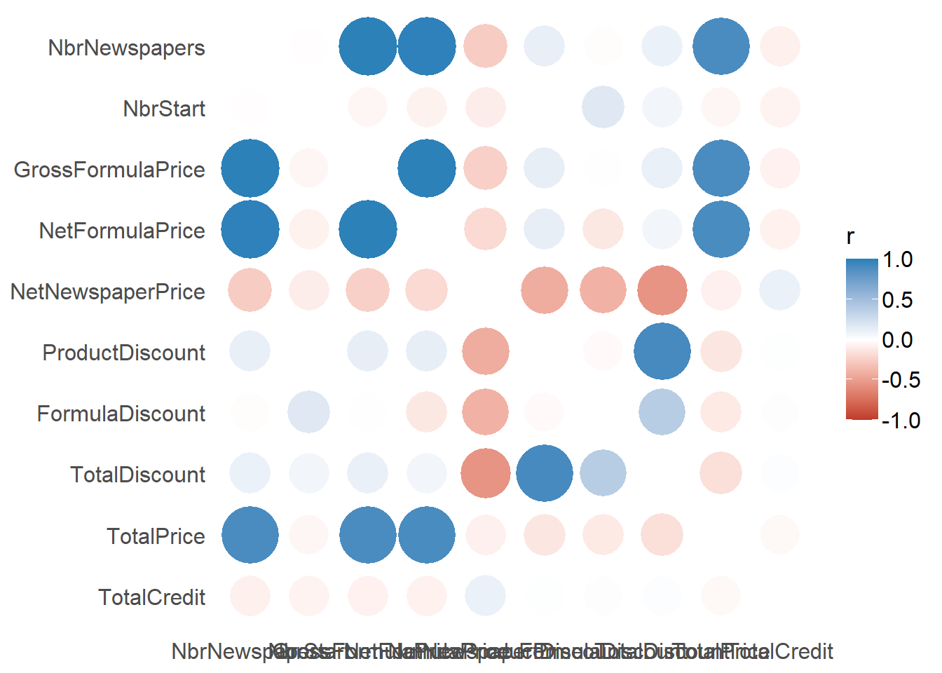
In slide 76, we saw a heuristic to delete highly correlated variables and hence solve multicollinearity. The idea is quite simple, you determine the two highest correlated variables, delete the one with highest average correlation with all other variables and repeat until your correlation is below the desired threshold. The findCorrelation function of the caret package implements this heuristic.
p_load(caret)

# The findCorrelation function will look at the mean
# absolute correlation and remove the one the largest one
# It takes the correlation matrix as an input The cutoff is
# the desired max amount of correlation Exact = FALSE,
# which will not re-evaluated the correlation at each step
(highCorr <- findCorrelation(corr, cutoff = 0.75, verbose = TRUE,
    names = TRUE, exact = FALSE))
##
## Combination row 1 and column 3 is above the cut-off, value = 0.993
## Flagging column 3
## Combination row 1 and column 4 is above the cut-off, value = 0.988
## Flagging column 4
## Combination row 3 and column 4 is above the cut-off, value = 0.993
## Flagging column 4
## Combination row 6 and column 8 is above the cut-off, value = 0.915
## Flagging column 8
## Combination row 1 and column 9 is above the cut-off, value = 0.899
## Flagging column 1
## Combination row 3 and column 9 is above the cut-off, value = 0.895
## Flagging column 3
## Combination row 4 and column 9 is above the cut-off, value = 0.901
## Flagging column 4## [1] "GrossFormulaPrice" "NetFormulaPrice"
## [3] "TotalDiscount" "NbrNewspapers"# By setting exact = TRUE, the function will recalculate
# the average correlations at each step This will increase
# the computation time, and remove less predictors By
# default exact = TRUE if the number of predictors < 100
(highCorr <- findCorrelation(corr, cutoff = 0.75, verbose = TRUE,
names = TRUE, exact = TRUE))## Compare row 4 and column 3 with corr 0.993
## Means: 0.392 vs 0.236 so flagging column 4
## Compare row 3 and column 1 with corr 0.993
## Means: 0.311 vs 0.204 so flagging column 3
## Compare row 1 and column 9 with corr 0.899
## Means: 0.212 vs 0.186 so flagging column 1
## Compare row 8 and column 6 with corr 0.915
## Means: 0.35 vs 0.169 so flagging column 8
## All correlations <= 0.75## [1] "NetFormulaPrice" "GrossFormulaPrice"
## [3] "NbrNewspapers" "TotalDiscount"Since there are better ways of selecting features, we will not remove these highly correlated variables at this stage
2.1.4.2 Missing values
# There is no built-in function in R to see all the missing
# values at once However, with 1 line of code you can
# easily spot the number of missing values
colSums(is.na(subscriptions))
## SubscriptionID CustomerID
## 0 0
## ProductID Pattern
## 0 0
## StartDate EndDate
## 0 0
## NbrNewspapers NbrStart
## 0 21
## RenewalDate PaymentType
## 2020 0
## PaymentStatus PaymentDate
## 0 421
## FormulaID GrossFormulaPrice
## 0 161
## NetFormulaPrice NetNewspaperPrice
## 161 161
## ProductDiscount FormulaDiscount
## 161 161
## TotalDiscount TotalPrice
## 161 161
## TotalCredit
## 161colSums(is.na(customers))## CustomerID Gender DOB District
## 0 0 0 0
## ZIP StreeID
## 0 0Remember that in order to handle missing values, you should always consider the cause of the missing values.
Also the number of missing values is important, if a variable has too many missing value it is better to remove them.
For example, in the case of RenewalDate deleting the variable might be better. Another solution can be to just add an indicator whether or not there was a renewal (which is the same as adding an indicator for NA).
However, handling your missing values at this point in time is not a good idea. It is better to perform your missing value imputation on the final basetable. So you should first calculate your dependent varables, compute your predictors and merge the tables. At the time of merging, be cautious that you treat missing values due to the merges differently!
Before imputing our missing values, we will perform several preprocessing steps. Note that I will not show you these preprocessing steps at this stage. In one of the exercises, you will have to perform these steps yourself. It is a good exercise for yourself to try these steps yourself and see whether your get the same result.
In this case we want to build a churn model, so the first thing that we have to do is determine our ‘churn’ variable. To determine churn, we first select the active subscriptions that can be targeted in the dependent period. This means those whose subscriptions end in the dependent period. Hence, active customers are those that have a start date before t2 and an end date in the dep (after t3 and before t4). We won’t consider them if they end after t4. We determine t1, t2, t3, t4 as follows:
f <- "%d/%m/%Y"
start_ind <- as.Date("02/01/2006", f)
end_ind <- as.Date("01/06/2009", f)
start_dep <- as.Date("02/06/2009", f)
end_dep <- as.Date("02/06/2010", f)  #dump date
length_ind <- end_ind - start_ind
After setting the time window, we should define churners as active customers who did not buy something in the dependent period. After having established the churn variable, we can compute several variables per customer However, you should only calculate your variables wit respect to the time window! So the idea will be to set your time window and only select active customers and compute variables on the subscriptions and customer table and finally join them together.
Since we are interested in preprocessing some variables at a later stage, we will only compute variables for the subscriptions table and not treat the dummies in the customer table (this will be done later in the preprocessing step). The resulting table of the data preprocessing can be found below:
# Load the data
load("SubCust.Rdata")

# Let's have a look at the data
SubCust %>%
    glimpse()
## Rows: 1,178
## Columns: 40
## $ CustomerID <chr> "100139", "10~
## $ ProductID_1_sum <int> 0, 0, 0, 0, 0~
## $ ProductID_2_sum <int> 0, 0, 0, 1, 0~
## $ ProductID_3_sum <int> 0, 0, 0, 0, 1~
## $ ProductID_4_sum <int> 0, 0, 0, 0, 0~
## $ ProductID_5_sum <int> 0, 0, 0, 0, 0~
## $ ProductID_6_sum <int> 0, 0, 0, 0, 0~
## $ ProductID_7_sum <int> 0, 0, 2, 0, 0~
## $ ProductID_8_sum <int> 5, 3, 0, 0, 0~
## $ Pattern_0000010_sum <int> 0, 0, 1, 0, 0~
## $ Pattern_0000100_sum <int> 0, 0, 0, 0, 0~
## $ Pattern_0001000_sum <int> 0, 0, 0, 0, 0~
## $ Pattern_0010000_sum <int> 0, 0, 0, 0, 0~
## $ Pattern_0100010_sum <int> 0, 0, 0, 0, 0~
## $ Pattern_1000010_sum <int> 0, 0, 0, 0, 0~
## $ Pattern_1001010_sum <int> 0, 0, 0, 0, 0~
## $ Pattern_1111110_sum <int> 5, 3, 1, 1, 1~
## $ PaymentType_BT_sum <int> 5, 3, 2, 1, 1~
## $ PaymentType_DD_sum <int> 0, 0, 0, 0, 0~
## $ PaymentStatus_Paid_sum <int> 5, 3, 2, 1, 1~
## $ PaymentStatus_Not.Paid_sum <int> 0, 0, 0, 0, 0~
## $ StartDate_rec <dbl> 152, 152, 107~
## $ RenewalDate_rec <dbl> 192, 192, NA,~
## $ PaymentDate_rec <dbl> 173, 167, 89,~
## $ NbrNewspapers_mean <dbl> 152.0, 304.0,~
## $ NbrStart_mean <dbl> 16, 15, 12, 2~
## $ GrossFormulaPrice_mean <dbl> 134.8000, 247~
## $ NetFormulaPrice_mean <dbl> 134.8000, 247~
## $ NetNewspaperPrice_mean <dbl> 0.8868566, 0.~
## $ ProductDiscount_mean <dbl> 0, 0, 0, 0, 0~
## $ FormulaDiscount_mean <dbl> 0.00, 0.00, 6~
## $ TotalDiscount_mean <dbl> 0.00, 0.00, 6~
## $ TotalPrice_mean <dbl> 134.8000, 247~
## $ TotalCredit_mean <dbl> 0.0, 0.0, 0.0~
## $ Gender <fct> M, M, M, M, M~
## $ District <fct> 5, 5, 1, 1, 1~
## $ ZIP <chr> "3740", "3740~
## $ StreeID <chr> "44349", "444~
## $ Age <dbl> 46, 76, 51, 7~
## $ churn <fct> 0, 0, 1, 1, 1~In sum, for the subscriptions table, I have taken the mean of all continuous variables per customer.
If a certain value had an NA, I just removed the NAs from the computation. A customer can have more than one subscription, so you should summarize this per customer. For the discrete variables, I have taken the sum per customer
and for the date variables I calculated the recency.Finally, I merged all tables together with the dependent variable.
Let’s now have a look at the NAs.
colSums(is.na(SubCust))## CustomerID
## 0
## ProductID_1_sum
## 0
## ProductID_2_sum
## 0
## ProductID_3_sum
## 0
## ProductID_4_sum
## 0
## ProductID_5_sum
## 0
## ProductID_6_sum
## 0
## ProductID_7_sum
## 0
## ProductID_8_sum
## 0
## Pattern_0000010_sum
## 0
## Pattern_0000100_sum
## 0
## Pattern_0001000_sum
## 0
## Pattern_0010000_sum
## 0
## Pattern_0100010_sum
## 0
## Pattern_1000010_sum
## 0
## Pattern_1001010_sum
## 0
## Pattern_1111110_sum
## 0
## PaymentType_BT_sum
## 0
## PaymentType_DD_sum
## 0
## PaymentStatus_Paid_sum
## 0
## PaymentStatus_Not.Paid_sum
## 0
## StartDate_rec
## 0
## RenewalDate_rec
## 154
## PaymentDate_rec
## 4
## NbrNewspapers_mean
## 0
## NbrStart_mean
## 0
## GrossFormulaPrice_mean
## 0
## NetFormulaPrice_mean
## 0
## NetNewspaperPrice_mean
## 0
## ProductDiscount_mean
## 0
## FormulaDiscount_mean
## 0
## TotalDiscount_mean
## 0
## TotalPrice_mean
## 0
## TotalCredit_mean
## 0
## Gender
## 211
## District
## 0
## ZIP
## 0
## StreeID
## 0
## Age
## 0
## churn
## 0colSums(is.na(SubCust))/nrow(SubCust)## CustomerID
## 0.000000000
## ProductID_1_sum
## 0.000000000
## ProductID_2_sum
## 0.000000000
## ProductID_3_sum
## 0.000000000
## ProductID_4_sum
## 0.000000000
## ProductID_5_sum
## 0.000000000
## ProductID_6_sum
## 0.000000000
## ProductID_7_sum
## 0.000000000
## ProductID_8_sum
## 0.000000000
## Pattern_0000010_sum
## 0.000000000
## Pattern_0000100_sum
## 0.000000000
## Pattern_0001000_sum
## 0.000000000
## Pattern_0010000_sum
## 0.000000000
## Pattern_0100010_sum
## 0.000000000
## Pattern_1000010_sum
## 0.000000000
## Pattern_1001010_sum
## 0.000000000
## Pattern_1111110_sum
## 0.000000000
## PaymentType_BT_sum
## 0.000000000
## PaymentType_DD_sum
## 0.000000000
## PaymentStatus_Paid_sum
## 0.000000000
## PaymentStatus_Not.Paid_sum
## 0.000000000
## StartDate_rec
## 0.000000000
## RenewalDate_rec
## 0.130730051
## PaymentDate_rec
## 0.003395586
## NbrNewspapers_mean
## 0.000000000
## NbrStart_mean
## 0.000000000
## GrossFormulaPrice_mean
## 0.000000000
## NetFormulaPrice_mean
## 0.000000000
## NetNewspaperPrice_mean
## 0.000000000
## ProductDiscount_mean
## 0.000000000
## FormulaDiscount_mean
## 0.000000000
## TotalDiscount_mean
## 0.000000000
## TotalPrice_mean
## 0.000000000
## TotalCredit_mean
## 0.000000000
## Gender
## 0.179117148
## District
## 0.000000000
## ZIP
## 0.000000000
## StreeID
## 0.000000000
## Age
## 0.000000000
## churn
## 0.000000000# Only 3 variables have NAs: payment date, renewal date and
# genderAs mentioned in the slides, there are two options:
-delete the columns: this can maybe be done for renewal date, however gender is a very important variable in every churn model, so should not be negelected. Also the number of NAs is acceptable, so we choose imputation.
-impute the values with the median(continuous)/mode(discrete) or impute with a model (e.g., random forest).
We will chose for imputation and therefore we will use the imputeMissing package.
# To impute variables, install the package imputeMissings
p_load(imputeMissings)

# This package is especially designed for a predictive
# context It allows you to compute the values on a training
# dataset and impute them on new data. This is very
# convenient in predictive contexts.

# For example: define training data
(train <- data.frame(v_int = as.integer(c(3, 3, 2, 5, 1, 2, 4,
    6)), v_num = as.numeric(c(4.1, NA, 12.2, 11, 3.4, 1.6, 3.3,
    5.5)), v_fact = as.factor(c("one", "two", NA, "two", "two",
    "one", "two", "two")), stringsAsFactors = FALSE))
## v_int v_num v_fact
## 1 3 4.1 one
## 2 3 NA two
## 3 2 12.2 <NA>
## 4 5 11.0 two
## 5 1 3.4 two
## 6 2 1.6 one
## 7 4 3.3 two
## 8 6 5.5 two# Compute values on train data randomForest method
values <- compute(train, method = "randomForest")
# median/mode method
(values2 <- compute(train))## $v_int
## [1] 3
##
## $v_num
## [1] 4.1
##
## $v_fact
## [1] "two"# define new data
(newdata <- data.frame(v_int = as.integer(c(1, 1, 2, NA)), v_num = as.numeric(c(1.1,
NA, 2.2, NA)), v_fact = as.factor(c("one", "one", "one",
NA)), stringsAsFactors = FALSE))## v_int v_num v_fact
## 1 1 1.1 one
## 2 1 NA one
## 3 2 2.2 one
## 4 NA NA <NA># locate the NA's
is.na(newdata)## v_int v_num v_fact
## [1,] FALSE FALSE FALSE
## [2,] FALSE TRUE FALSE
## [3,] FALSE FALSE FALSE
## [4,] TRUE TRUE TRUE# how many missings per variable?
colSums(is.na(newdata))## v_int v_num v_fact
## 1 2 1# Impute on newdata using the previously created object
imputeMissings::impute(newdata, object = values) #using randomForest values## v_int v_num v_fact
## 1 1.000000 1.1000 one
## 2 1.000000 3.9814 one
## 3 2.000000 2.2000 one
## 4 2.456469 3.9814 oneimputeMissings::impute(newdata, object = values2) #using median/mode values## v_int v_num v_fact
## 1 1 1.1 one
## 2 1 4.1 one
## 3 2 2.2 one
## 4 3 4.1 two# One can also impute directly in newdata without the
# compute step
imputeMissings::impute(newdata)## v_int v_num v_fact
## 1 1 1.10 one
## 2 1 1.65 one
## 3 2 2.20 one
## 4 1 1.65 one# It may be useful to have indicators for the variables
# imputations. These indicators may be predictive. To
# create these indicators, use flag=TRUE
# Flag parameter
imputeMissings::impute(newdata, flag = TRUE)## v_int v_num v_fact v_int_flag v_num_flag
## 1 1 1.10 one 0 0
## 2 1 1.65 one 0 1
## 3 2 2.20 one 0 0
## 4 1 1.65 one 1 1
## v_fact_flag
## 1 0
## 2 0
## 3 0
## 4 1Now let’s apply this missing value imputation to our data. There is , however, one problem. Ideally imputation should be done on the training set and the same values should be used on the test set. This means that we should first split our data into training and test and we can then perform missing value imputation.
# Split in train and test using a 50/50 split Set the same
# seed to have the same splits
set.seed(100)

ind <- sample(x = nrow(SubCust), size = round(0.5 * nrow(SubCust)),
    replace = FALSE)
train <- SubCust[ind, ]
test <- SubCust[-ind, ]
# You can also save the data to make sture you get the same
# splits save(train,test, file = 'SubCust_traintest.Rdata')

# I have already created the data for you, so you can just
# load the data to make sure you are using the same splits
# load('SubCust_traintest.Rdata')

# Let's compute the values with on the training set
# randomForest method: make sure you delete the churn
# variable, the customerID and characters variables (ZIP,
# StreeID) values <- compute(data = train[,!names(train)
# %in% c('churn', 'CustomerID', 'ZIP', 'StreeID')],
# method='randomForest') As can be noticed, the random
# forest procedure takes quite some time (we did not run it
# for the compilation of this book) this is because the
# function calculates a random forest for all variables

# calculating the median/mode is a lot faster In most churn
# literature, the median/mode is preferred, so this will
# also be our preferred option
values2 <- compute(train)

# impute the train and test data with the imputation values
# also add a flag for missing values
train_imp <- imputeMissings::impute(train, object = values2,
    flag = TRUE)
test_imp <- imputeMissings::impute(test, object = values2, flag = TRUE)

colSums(is.na(train_imp))
## CustomerID
## 0
## ProductID_1_sum
## 0
## ProductID_2_sum
## 0
## ProductID_3_sum
## 0
## ProductID_4_sum
## 0
## ProductID_5_sum
## 0
## ProductID_6_sum
## 0
## ProductID_7_sum
## 0
## ProductID_8_sum
## 0
## Pattern_0000010_sum
## 0
## Pattern_0000100_sum
## 0
## Pattern_0001000_sum
## 0
## Pattern_0010000_sum
## 0
## Pattern_0100010_sum
## 0
## Pattern_1000010_sum
## 0
## Pattern_1001010_sum
## 0
## Pattern_1111110_sum
## 0
## PaymentType_BT_sum
## 0
## PaymentType_DD_sum
## 0
## PaymentStatus_Paid_sum
## 0
## PaymentStatus_Not.Paid_sum
## 0
## StartDate_rec
## 0
## RenewalDate_rec
## 0
## PaymentDate_rec
## 0
## NbrNewspapers_mean
## 0
## NbrStart_mean
## 0
## GrossFormulaPrice_mean
## 0
## NetFormulaPrice_mean
## 0
## NetNewspaperPrice_mean
## 0
## ProductDiscount_mean
## 0
## FormulaDiscount_mean
## 0
## TotalDiscount_mean
## 0
## TotalPrice_mean
## 0
## TotalCredit_mean
## 0
## Gender
## 0
## District
## 0
## ZIP
## 0
## StreeID
## 0
## Age
## 0
## churn
## 0
## RenewalDate_rec_flag
## 0
## PaymentDate_rec_flag
## 0
## Gender_flag
## 0colSums(is.na(test_imp))## CustomerID
## 0
## ProductID_1_sum
## 0
## ProductID_2_sum
## 0
## ProductID_3_sum
## 0
## ProductID_4_sum
## 0
## ProductID_5_sum
## 0
## ProductID_6_sum
## 0
## ProductID_7_sum
## 0
## ProductID_8_sum
## 0
## Pattern_0000010_sum
## 0
## Pattern_0000100_sum
## 0
## Pattern_0001000_sum
## 0
## Pattern_0010000_sum
## 0
## Pattern_0100010_sum
## 0
## Pattern_1000010_sum
## 0
## Pattern_1001010_sum
## 0
## Pattern_1111110_sum
## 0
## PaymentType_BT_sum
## 0
## PaymentType_DD_sum
## 0
## PaymentStatus_Paid_sum
## 0
## PaymentStatus_Not.Paid_sum
## 0
## StartDate_rec
## 0
## RenewalDate_rec
## 0
## PaymentDate_rec
## 0
## NbrNewspapers_mean
## 0
## NbrStart_mean
## 0
## GrossFormulaPrice_mean
## 0
## NetFormulaPrice_mean
## 0
## NetNewspaperPrice_mean
## 0
## ProductDiscount_mean
## 0
## FormulaDiscount_mean
## 0
## TotalDiscount_mean
## 0
## TotalPrice_mean
## 0
## TotalCredit_mean
## 0
## Gender
## 0
## District
## 0
## ZIP
## 0
## StreeID
## 0
## Age
## 0
## churn
## 0
## RenewalDate_rec_flag
## 0
## PaymentDate_rec_flag
## 0
## Gender_flag
## 02.1.4.3 Outliers
Outliers can be detected and treated in different ways: graphically or statistically (e.g., Z-scores). We will focus on one of the most common ways to spot outliers: box plots and histograms.
Note that for the plotting, we will using the pivot_longer function, which transforms the data from a wide to a long format. This can come in very handy when plotting, you might have a look at this blogpost https://thatdatatho.com/2020/03/28/tidyrs-pivot_longer-and-pivot_wider-examples-tidytuesday-challenge/ tp see how pivoting works in R. The tidyr website also contains some good examples, to get you more familar with the coding style: https://tidyr.tidyverse.org/articles/pivot.html.
#Outliers are mainly related to continuous variables, so let's plot all
#outliers for al numerics
#Again, this will only be done on the training data and the same rule
#will be applied to the test data
num <- train_imp %>% select_if(is.numeric)

#Boxplots
#For easy plotting, we will transform the table from a wide to a long format
#using pivot_longer
#This means that instead of using one column for every variable,


#This is how the wide table looks like: one column for every variable
num %>% head()
## ProductID_1_sum ProductID_2_sum
## 503 0 0
## 985 0 0
## 1004 0 1
## 919 0 0
## 470 0 0
## 823 0 0
## ProductID_3_sum ProductID_4_sum
## 503 0 0
## 985 0 0
## 1004 0 2
## 919 0 0
## 470 0 0
## 823 0 0
## ProductID_5_sum ProductID_6_sum
## 503 0 0
## 985 0 0
## 1004 0 0
## 919 0 3
## 470 0 0
## 823 0 0
## ProductID_7_sum ProductID_8_sum
## 503 0 4
## 985 0 2
## 1004 0 0
## 919 0 0
## 470 0 4
## 823 0 3
## Pattern_0000010_sum Pattern_0000100_sum
## 503 0 0
## 985 0 0
## 1004 0 0
## 919 0 0
## 470 0 0
## 823 0 0
## Pattern_0001000_sum Pattern_0010000_sum
## 503 0 0
## 985 0 0
## 1004 0 0
## 919 0 0
## 470 0 0
## 823 0 0
## Pattern_0100010_sum Pattern_1000010_sum
## 503 0 0
## 985 0 0
## 1004 0 0
## 919 0 0
## 470 0 0
## 823 0 0
## Pattern_1001010_sum Pattern_1111110_sum
## 503 0 4
## 985 0 2
## 1004 0 3
## 919 0 3
## 470 0 4
## 823 0 3
## PaymentType_BT_sum PaymentType_DD_sum
## 503 4 0
## 985 2 0
## 1004 3 0
## 919 3 0
## 470 4 0
## 823 3 0
## PaymentStatus_Paid_sum
## 503 4
## 985 2
## 1004 3
## 919 3
## 470 4
## 823 3
## PaymentStatus_Not.Paid_sum StartDate_rec
## 503 0 62
## 985 0 78
## 1004 0 359
## 919 0 318
## 470 0 86
## 823 0 96
## RenewalDate_rec PaymentDate_rec
## 503 91 68
## 985 101 53
## 1004 390 370
## 919 349 339
## 470 117 105
## 823 126 115
## NbrNewspapers_mean NbrStart_mean
## 503 310.2500 15.00000
## 985 46.5000 7.50000
## 1004 304.6667 16.66667
## 919 313.0000 16.66667
## 470 304.0000 15.00000
## 823 219.3333 15.00000
## GrossFormulaPrice_mean NetFormulaPrice_mean
## 503 247.7075 243.0000
## 985 45.1000 45.1000
## 1004 237.6667 237.6667
## 919 237.6667 237.6667
## 470 243.0000 243.0000
## 823 185.5600 168.7067
## NetNewspaperPrice_mean ProductDiscount_mean
## 503 0.7850320 0.00000
## 985 0.9647820 1.56055
## 1004 0.7801140 0.00000
## 919 0.7599373 0.00000
## 470 0.7993303 0.00000
## 823 0.7109210 0.00000
## FormulaDiscount_mean TotalDiscount_mean
## 503 4.70750 4.70750
## 985 0.00000 1.56055
## 1004 0.00000 0.00000
## 919 0.00000 0.00000
## 470 0.00000 0.00000
## 823 16.85333 16.85333
## TotalPrice_mean TotalCredit_mean Age
## 503 243.0000 0.0000000 61
## 985 38.5000 -7.7894500 61
## 1004 237.6667 0.0000000 55
## 919 237.3333 -0.3333333 57
## 470 243.0000 0.0000000 61
## 823 168.7067 0.0000000 60#This is how the long table looks like:
#the column names will be casted into one variable called 'variable'
#and the corresponding values will be casted into a 'value' variable
#So now you will have only two columns variable and value but with
#20,026 observations (584 obs * 34 variables)
#See: https://tidyr.tidyverse.org/index.html for more information
num %>%
pivot_longer(everything(),names_to = "variable", values_to = "value") %>%
head(n = 20)## # A tibble: 20 x 2
## variable value
## <chr> <dbl>
## 1 ProductID_1_sum 0
## 2 ProductID_2_sum 0
## 3 ProductID_3_sum 0
## 4 ProductID_4_sum 0
## 5 ProductID_5_sum 0
## 6 ProductID_6_sum 0
## 7 ProductID_7_sum 0
## 8 ProductID_8_sum 4
## 9 Pattern_0000010_sum 0
## 10 Pattern_0000100_sum 0
## 11 Pattern_0001000_sum 0
## 12 Pattern_0010000_sum 0
## 13 Pattern_0100010_sum 0
## 14 Pattern_1000010_sum 0
## 15 Pattern_1001010_sum 0
## 16 Pattern_1111110_sum 4
## 17 PaymentType_BT_sum 4
## 18 PaymentType_DD_sum 0
## 19 PaymentStatus_Paid_sum 4
## 20 PaymentStatus_Not.Paid_sum 0#Plot the boxplot in one tidy command
num %>%
pivot_longer(everything(),names_to = "variable", values_to = "value") %>%
ggplot(aes(x = variable, y = value)) + geom_boxplot() +
facet_wrap(~variable, scales = "free")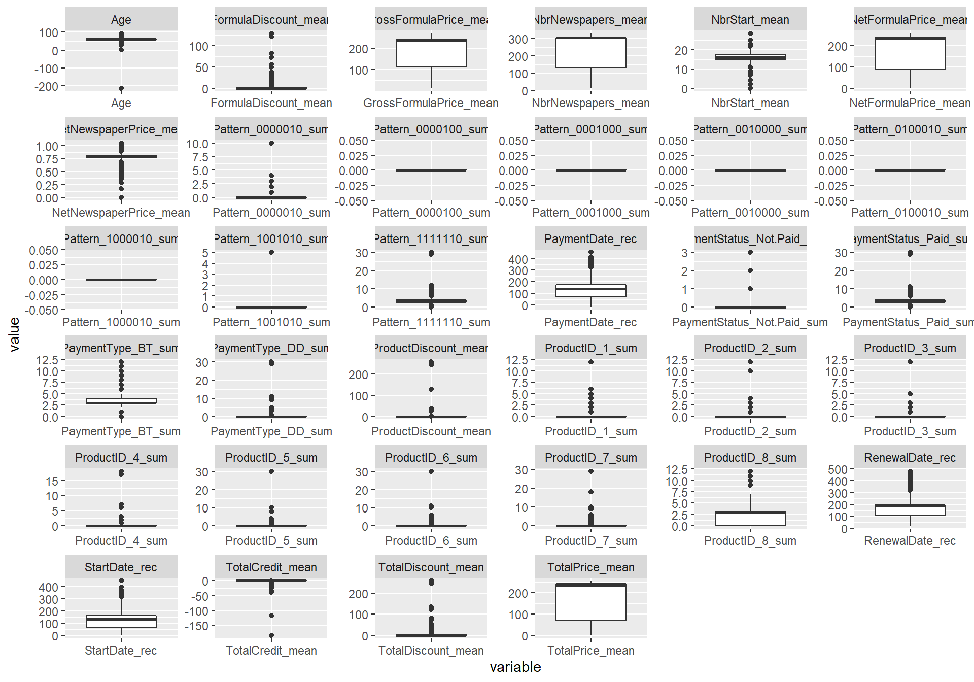
#While boxplots are clear visualizations, some of you may prefer violin plots
#If you would want a violin plot, just state: geom_violin

#Histograms
num %>%
  pivot_longer(everything(),names_to = "variable", values_to = "value") %>%
  ggplot(aes(x = value)) + geom_histogram() +
  facet_wrap(~variable, scales = "free")
## `stat_bin()` using `bins = 30`. Pick better
## value with `binwidth`.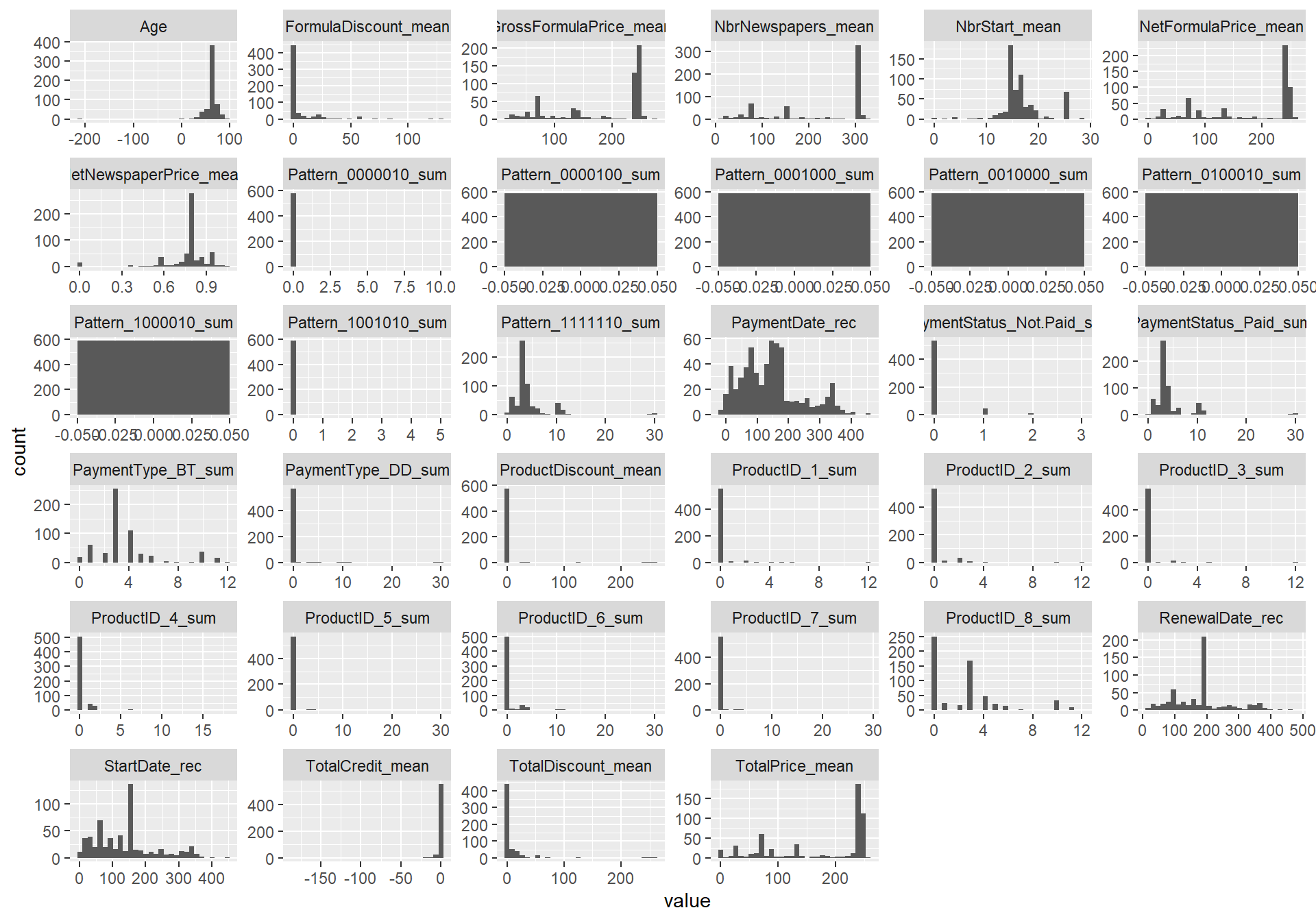
#When looking at the boxplots, you might believe that there are many outliers
#However, when looking at the histograms, things don't seem that odd
#So we might assume that these observations are just valid and maybe coming from
#another skewed distribution
#The only odd thing is the negative age

#So the idea is to set this to NA and impute with the median (of the training set!)
train_imp$Age <- ifelse(train_imp$Age < 0, NA,train_imp$Age)
train_imp$Age <- ifelse(is.na(train_imp$Age),
                        median(train_imp$Age, na.rm = TRUE), train_imp$Age)
test_imp$Age <- ifelse(test_imp$Age < 0,
                       median(train_imp$Age, na.rm = TRUE), test_imp$Age)

#Let's replot the age variable to see whether everything is correct
qplot(train_imp$Age)
## `stat_bin()` using `bins = 30`. Pick better
## value with `binwidth`.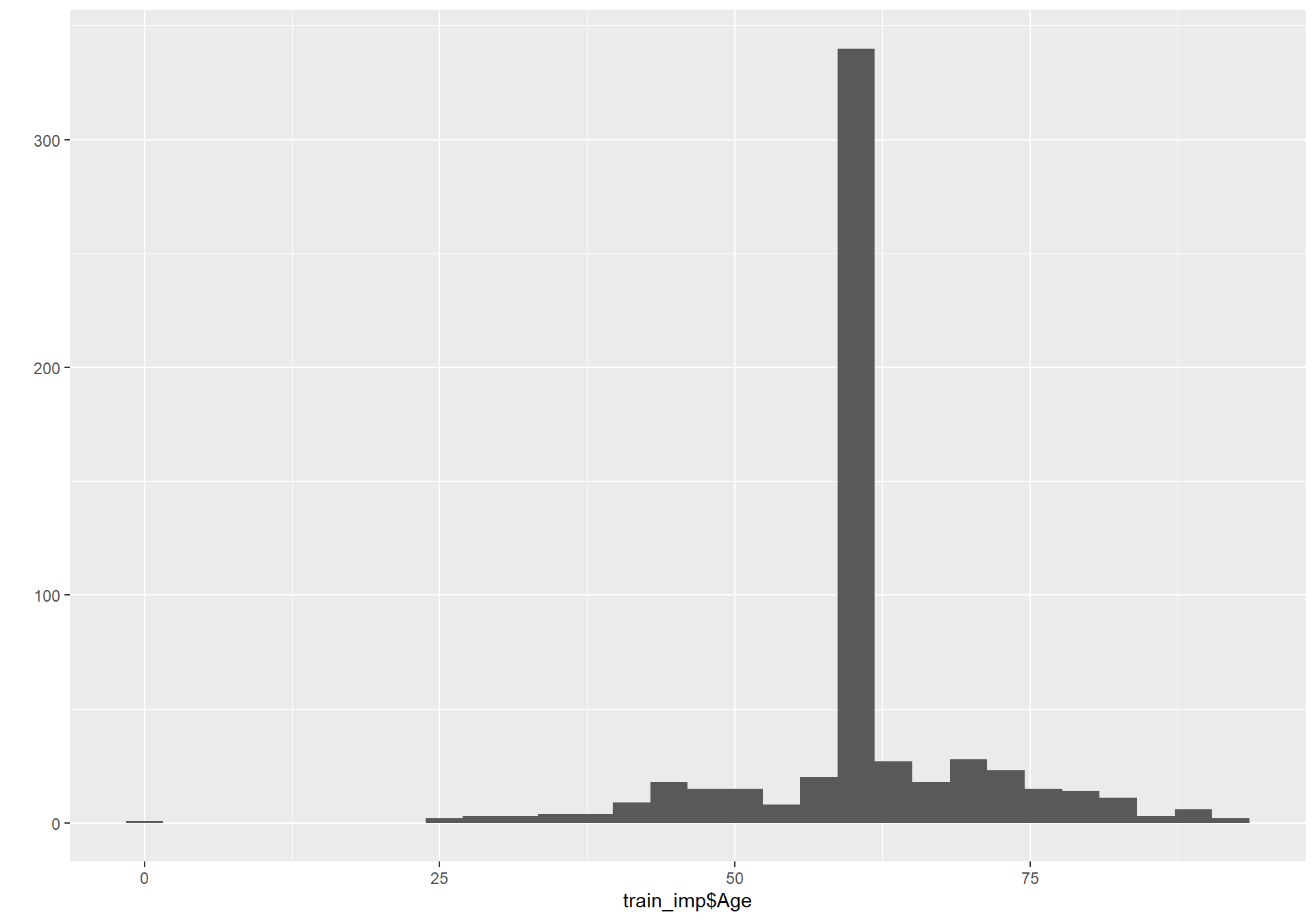
#Apparantly there is is also someone with a very young age, let's just leave it
#like this at this point.

#Let's save our train and test data after solving the data quality issues
save(train_imp,test_imp, file = 'SubCust_traintest_preparation.Rdata')
2.2 Data preparation
To make sure that we are using the same data, let’s load our saved data set.
# Load the data
load("SubCust_traintest_preparation.Rdata")
In this section, we will look into some specific value transformations, representations, feature engineering and variable selection methods.
2.2.1 Value transformations
Let’s look into some specific value transformation. Note that we will not use standardizing or normalization here because this can impact feature engineering at a later stage.
Continuous categorization
Continuous categorization will categoize numeric variables into bins. A very good package to perform binning in R is the rbin package (see: https://github.com/rsquaredacademy/rbin).
p_load(rbin)

# For example, let's bin the age variable, as this is often
# done in churn modeling Equal frequency binning
bin <- rbin_equal_freq(data = train_imp, response = churn, predictor = Age,
    bins = 10)
bin
## Binning Summary
## ------------------------------------
## Method Equal Frequency
## Response churn
## Predictor Age
## Bins 10
## Count 589
## Goods 152
## Bads 437
## Entropy 0.81
## Information Value 0.07
##
##
## lower_cut upper_cut bin_count good bad
## 1 1 49 59 16 43
## 2 50 61 59 10 49
## 3 61 61 59 19 40
## 4 61 61 59 13 46
## 5 61 61 59 17 42
## 6 61 61 59 14 45
## 7 61 61 59 16 43
## 8 61 66 59 11 48
## 9 66 74 58 17 41
## 10 74 93 59 19 40
## good_rate woe iv entropy
## 1 0.2711864 -0.06744128 0.0004629836 0.8431620
## 2 0.1694915 0.53318253 0.0247069708 0.6565403
## 3 0.3220339 -0.31161220 0.0104286691 0.9065795
## 4 0.2203390 0.20763936 0.0040981454 0.7607860
## 5 0.2881356 -0.15159640 0.0023849548 0.8663007
## 6 0.2372881 0.11155249 0.0012125270 0.7905014
## 7 0.2711864 -0.06744128 0.0004629836 0.8431620
## 8 0.1864407 0.41725306 0.0156350547 0.6939660
## 9 0.2931034 -0.17569395 0.0031661095 0.8726965
## 10 0.3220339 -0.31161220 0.0104286691 0.9065795# A cool thing about the function is that it also shows you
# the WOE and IV for your binning exercise Hence, you can
# already see whether the binning has a good effect on
# predictive value Remember that a good rule-of-thumb is an
# IV>0.10
# You can also make a WOE plot to see the the effect of
# each age category Remember that a positive WOE means that
# there are more events (1) than non-events (0)
# The current package version is still a little buggy,
# which is why you get the same plot twice if you call the
# plot function on your binning object and why the 10th is
# perhaps placed rather unclear on the plot
# Nevertheless, the plot allows for a quick interpretation
# of the effect of your binning on the dependent variable.
plot(bin)
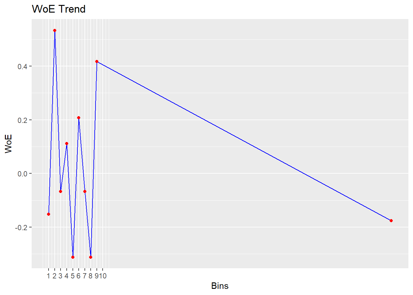
# Looking at the IVs and the plot, binning is not such a
# good idea ...

# Equal interval/width binning Because there are a lot of
# elderly people a lot of equal length bins is impossible
bin <- rbin_equal_length(data = train_imp, response = churn,
    predictor = Age, bins = 3)
bin
## Binning Summary
## ---------------------------------
## Method Equal Length
## Response churn
## Predictor Age
## Bins 3
## Count 589
## Goods 152
## Bads 437
## Entropy 0.82
## Information Value 0.03
##
##
## cut_point bin_count good bad
## 1 < 31.6666666666667 8 4 4
## 2 < 62.3333333333333 438 117 321
## 3 >= 62.3333333333333 143 31 112
## woe iv entropy
## 1 -1.05605267 0.018124474 1.0000000
## 2 -0.04678549 0.001646057 0.8373064
## 3 0.22845899 0.011958809 0.7542501plot(bin)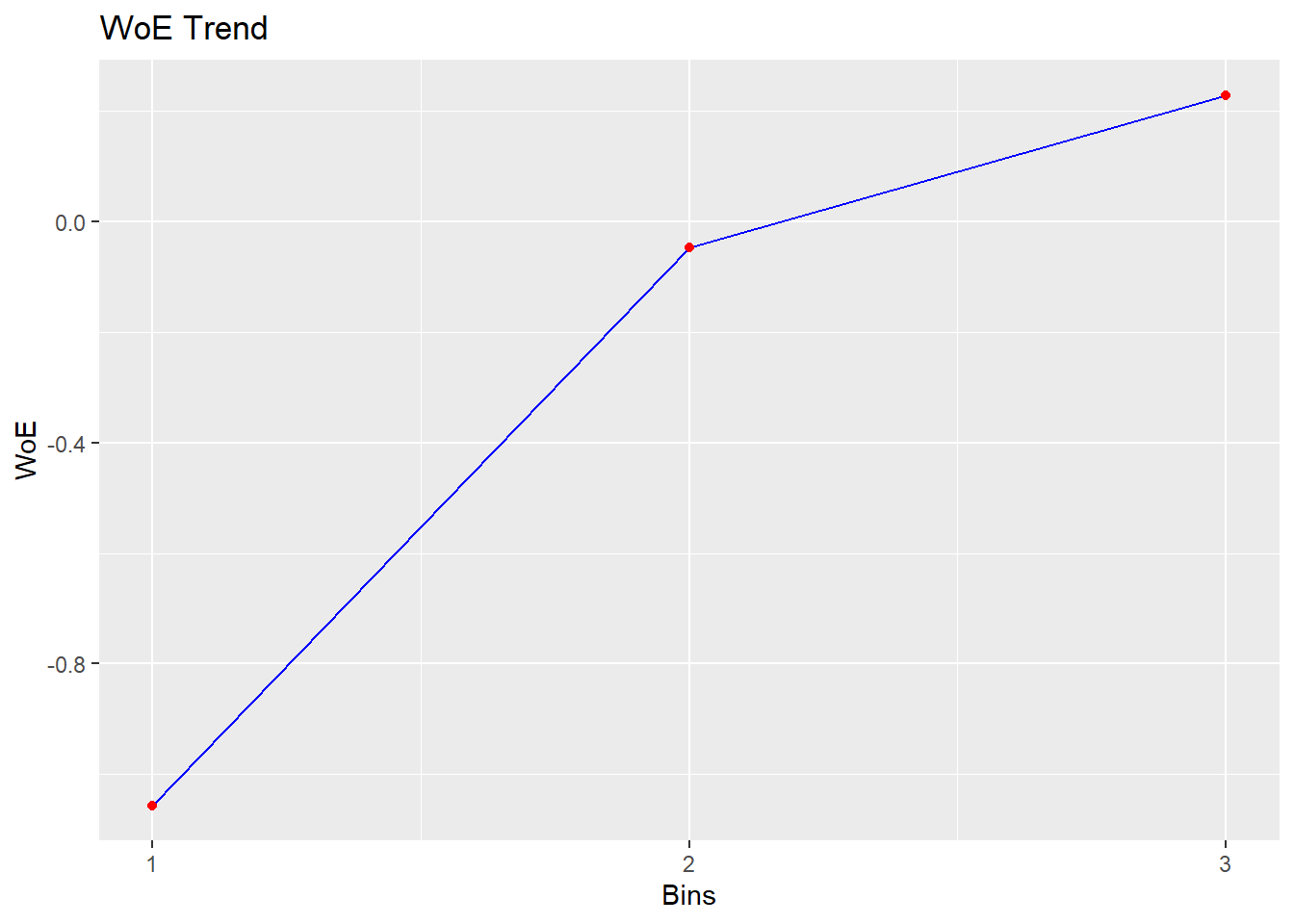

# The trend is more clear in this case, but the IV is still
# low So let's keep it like this for now
Discrete categorization
Binning discrete variables is a bit more difficult in R and not all packages support factors. One of the best packages available is woeBinning. This package bins discrete and numeric (!) variables in an automated fashion: categories will be joined together as long as the information value is not decreased by a certain factor, in the end the optimal solution in terms of IV is shown. Furthermore, it also has support for a predictive context, so in that sense it is superior to the rbin package.
The workhorse function is woe.binning, which allows you to bin one variable, two variables or even all variables. It also allows you to perform Laplacian smoothing to handle 0 frequencies.
Let’s work out an example on the District variable.
p_load(woeBinning)

# ?woe.binning Min.perc.total = 0.05 This parameter defines
# the number of initial classes before any merging is
# applied for numeric variables (0.05 implies 20 initial
# classes) this means that for factors that the original
# categories with less observations will be joined in
# 'miscellaneous' group stop.limit = 0.1 if the resulting
# IV decreases with more than 0.10, stop binning even.class
# = 1, this is the target class (in the package called
# negative event) that we predict (in our case churn)
binning <- woe.binning(train_imp, "churn", "District", min.perc.total = 0.05,
    min.perc.class = 0, stop.limit = 0.1, abbrev.fact.levels = 50,
    event.class = 1)

# Look at the solution
woe.binning.table(binning)
## $`WOE Table for District`
## Final.Bin Total.Count Total.Distr.
## 1 misc. level neg. 35 5.9%
## 2 5 + 1 552 93.7%
## 3 misc. level pos. 2 0.3%
## 4 Total 589 100.0%
## 0.Count 1.Count 0.Distr. 1.Distr. 1.Rate WOE
## 1 15 20 3.4% 13.2% 57.1% -134.2
## 2 420 132 96.1% 86.8% 23.9% 10.1
## 3 2 0 0.5% 0.0% 0.0% 384.5
## 4 437 152 100.0% 100.0% 25.8% NA
## IV
## 1 0.130
## 2 0.009
## 3 0.018
## 4 0.157woe.binning.plot(binning)
# We can see that the algorithm decided to join district 5
# and 1 The other categories are joined together in a Misc
# group for the negatives (churn) and the positives (no
# churn)
# Now we still need to add the binning solution to the data
# frame We can use the woe.binning.deploy function This can
# be used on the training and the test set, so very useful
# for predictive context You can also choose to add dummies
# (var = 'dum') or add woe (var = 'dum')
train_binned_district <- woe.binning.deploy(train_imp, binning,
add.woe.or.dum.var = "dum")
head(train_binned_district)## CustomerID ProductID_1_sum ProductID_2_sum
## 503 497954 0 0
## 985 855200 0 0
## 1004 870967 0 1
## 919 800576 0 0
## 470 459730 0 0
## 823 746052 0 0
## ProductID_3_sum ProductID_4_sum
## 503 0 0
## 985 0 0
## 1004 0 2
## 919 0 0
## 470 0 0
## 823 0 0
## ProductID_5_sum ProductID_6_sum
## 503 0 0
## 985 0 0
## 1004 0 0
## 919 0 3
## 470 0 0
## 823 0 0
## ProductID_7_sum ProductID_8_sum
## 503 0 4
## 985 0 2
## 1004 0 0
## 919 0 0
## 470 0 4
## 823 0 3
## Pattern_0000010_sum Pattern_0000100_sum
## 503 0 0
## 985 0 0
## 1004 0 0
## 919 0 0
## 470 0 0
## 823 0 0
## Pattern_0001000_sum Pattern_0010000_sum
## 503 0 0
## 985 0 0
## 1004 0 0
## 919 0 0
## 470 0 0
## 823 0 0
## Pattern_0100010_sum Pattern_1000010_sum
## 503 0 0
## 985 0 0
## 1004 0 0
## 919 0 0
## 470 0 0
## 823 0 0
## Pattern_1001010_sum Pattern_1111110_sum
## 503 0 4
## 985 0 2
## 1004 0 3
## 919 0 3
## 470 0 4
## 823 0 3
## PaymentType_BT_sum PaymentType_DD_sum
## 503 4 0
## 985 2 0
## 1004 3 0
## 919 3 0
## 470 4 0
## 823 3 0
## PaymentStatus_Paid_sum
## 503 4
## 985 2
## 1004 3
## 919 3
## 470 4
## 823 3
## PaymentStatus_Not.Paid_sum StartDate_rec
## 503 0 62
## 985 0 78
## 1004 0 359
## 919 0 318
## 470 0 86
## 823 0 96
## RenewalDate_rec PaymentDate_rec
## 503 91 68
## 985 101 53
## 1004 390 370
## 919 349 339
## 470 117 105
## 823 126 115
## NbrNewspapers_mean NbrStart_mean
## 503 310.2500 15.00000
## 985 46.5000 7.50000
## 1004 304.6667 16.66667
## 919 313.0000 16.66667
## 470 304.0000 15.00000
## 823 219.3333 15.00000
## GrossFormulaPrice_mean NetFormulaPrice_mean
## 503 247.7075 243.0000
## 985 45.1000 45.1000
## 1004 237.6667 237.6667
## 919 237.6667 237.6667
## 470 243.0000 243.0000
## 823 185.5600 168.7067
## NetNewspaperPrice_mean ProductDiscount_mean
## 503 0.7850320 0.00000
## 985 0.9647820 1.56055
## 1004 0.7801140 0.00000
## 919 0.7599373 0.00000
## 470 0.7993303 0.00000
## 823 0.7109210 0.00000
## FormulaDiscount_mean TotalDiscount_mean
## 503 4.70750 4.70750
## 985 0.00000 1.56055
## 1004 0.00000 0.00000
## 919 0.00000 0.00000
## 470 0.00000 0.00000
## 823 16.85333 16.85333
## TotalPrice_mean TotalCredit_mean Gender
## 503 243.0000 0.0000000 M
## 985 38.5000 -7.7894500 F
## 1004 237.6667 0.0000000 M
## 919 237.3333 -0.3333333 F
## 470 243.0000 0.0000000 M
## 823 168.7067 0.0000000 M
## District ZIP StreeID Age churn
## 503 5 3920 46886 61 1
## 985 5 3530 38415 61 1
## 1004 1 2930 29121 55 0
## 919 1 2430 20879 57 0
## 470 5 3640 42237 61 1
## 823 5 3670 43000 60 1
## RenewalDate_rec_flag PaymentDate_rec_flag
## 503 0 0
## 985 0 0
## 1004 0 0
## 919 0 0
## 470 0 0
## 823 0 0
## Gender_flag District.binned
## 503 0 5 + 1
## 985 0 5 + 1
## 1004 0 5 + 1
## 919 0 5 + 1
## 470 1 5 + 1
## 823 0 5 + 1
## dum.District.51.binned
## 503 1
## 985 1
## 1004 1
## 919 1
## 470 1
## 823 1
## dum.District.misclevelneg.binned
## 503 0
## 985 0
## 1004 0
## 919 0
## 470 0
## 823 0
## dum.District.misclevelpos.binned
## 503 0
## 985 0
## 1004 0
## 919 0
## 470 0
## 823 0# Just be sure the delete the District.binned variable and
# and the original District variable in the final solution
# Applying this on the test set, is straightforward
test_binned_district <- woe.binning.deploy(test_imp, binning,
add.woe.or.dum.var = "dum")
head(test_binned_district)## CustomerID ProductID_1_sum ProductID_2_sum
## 3 1004392 0 0
## 5 1005543 0 0
## 7 1005612 0 0
## 8 100579 0 0
## 10 1006986 0 0
## 15 1010541 2 0
## ProductID_3_sum ProductID_4_sum
## 3 0 0
## 5 1 0
## 7 1 0
## 8 0 0
## 10 0 0
## 15 0 0
## ProductID_5_sum ProductID_6_sum
## 3 0 0
## 5 0 0
## 7 0 0
## 8 0 0
## 10 0 0
## 15 0 0
## ProductID_7_sum ProductID_8_sum
## 3 2 0
## 5 0 0
## 7 0 0
## 8 0 3
## 10 1 0
## 15 0 0
## Pattern_0000010_sum Pattern_0000100_sum
## 3 1 0
## 5 0 0
## 7 0 0
## 8 0 0
## 10 0 0
## 15 0 0
## Pattern_0001000_sum Pattern_0010000_sum
## 3 0 0
## 5 0 0
## 7 0 0
## 8 0 0
## 10 0 0
## 15 0 0
## Pattern_0100010_sum Pattern_1000010_sum
## 3 0 0
## 5 0 0
## 7 0 0
## 8 0 0
## 10 0 0
## 15 0 0
## Pattern_1001010_sum Pattern_1111110_sum
## 3 0 1
## 5 0 1
## 7 0 1
## 8 0 3
## 10 0 1
## 15 0 2
## PaymentType_BT_sum PaymentType_DD_sum
## 3 2 0
## 5 1 0
## 7 1 0
## 8 3 0
## 10 1 0
## 15 2 0
## PaymentStatus_Paid_sum
## 3 2
## 5 1
## 7 1
## 8 3
## 10 1
## 15 1
## PaymentStatus_Not.Paid_sum StartDate_rec
## 3 0 107
## 5 0 123
## 7 0 123
## 8 0 152
## 10 0 123
## 15 1 105
## RenewalDate_rec PaymentDate_rec
## 3 189 89
## 5 189 124
## 7 189 124
## 8 192 166
## 10 189 125
## 15 189 96
## NbrNewspapers_mean NbrStart_mean
## 3 32 12
## 5 152 25
## 7 152 25
## 8 304 15
## 10 304 25
## 15 152 25
## GrossFormulaPrice_mean NetFormulaPrice_mean
## 3 34.8400 28.6000
## 5 144.0000 72.0000
## 7 144.0000 72.0000
## 8 247.6667 247.6667
## 10 249.0000 249.0000
## 15 144.0000 144.0000
## NetNewspaperPrice_mean ProductDiscount_mean
## 3 0.550000 0
## 5 0.473684 0
## 7 0.473684 0
## 8 0.814693 0
## 10 0.819079 0
## 15 0.947368 0
## FormulaDiscount_mean TotalDiscount_mean
## 3 6.24 6.24
## 5 72.00 72.00
## 7 72.00 72.00
## 8 0.00 0.00
## 10 0.00 0.00
## 15 0.00 0.00
## TotalPrice_mean TotalCredit_mean Gender
## 3 29.8400 0 M
## 5 72.0000 0 M
## 7 72.0000 0 M
## 8 247.6667 0 M
## 10 249.0000 0 M
## 15 144.0000 0 M
## District ZIP StreeID Age churn
## 3 1 2560 23762 51 1
## 5 1 2620 24963 61 1
## 7 1 2620 24901 24 1
## 8 5 3740 44455 61 0
## 10 2 3000 31086 61 0
## 15 1 2610 24672 61 0
## RenewalDate_rec_flag PaymentDate_rec_flag
## 3 1 0
## 5 1 0
## 7 1 0
## 8 0 0
## 10 1 0
## 15 1 0
## Gender_flag District.binned
## 3 0 5 + 1
## 5 0 5 + 1
## 7 0 5 + 1
## 8 1 5 + 1
## 10 1 misc. level neg.
## 15 1 5 + 1
## dum.District.51.binned
## 3 1
## 5 1
## 7 1
## 8 1
## 10 0
## 15 1
## dum.District.misclevelneg.binned
## 3 0
## 5 0
## 7 0
## 8 0
## 10 1
## 15 0
## dum.District.misclevelpos.binned
## 3 0
## 5 0
## 7 0
## 8 0
## 10 0
## 15 0There is also a function to perform decision tree mapping woe.tree.binning(). This function will build a tree that uses the the IV as a splitting criterion. The procedure will stop if the increase in IV is less than a certain percentage (stop.limit parameter).
binning_tree <- woe.tree.binning(train_imp, "churn", "District",
    min.perc.total = 0.05, min.perc.class = 0, stop.limit = 0.1,
    abbrev.fact.levels = 50, event.class = 1)

woe.binning.table(binning_tree)
## $`WOE Table for District`
## Final.Bin Total.Count Total.Distr.
## 1 misc. level neg. 35 5.9%
## 2 1 224 38.0%
## 3 5 + misc. level pos. 330 56.0%
## 4 Total 589 100.0%
## 0.Count 1.Count 0.Distr. 1.Distr. 1.Rate WOE
## 1 15 20 3.4% 13.2% 57.1% -134.4
## 2 160 64 36.6% 42.1% 28.6% -14.0
## 3 262 68 60.0% 44.7% 20.6% 29.3
## 4 437 152 100.0% 100.0% 25.8% NA
## IV
## 1 0.131
## 2 0.008
## 3 0.045
## 4 0.183woe.binning.plot(binning_tree)
# The solution is more or less the same, but with a higher
# IVAnother good package for decision tree mapping is the tree.bins package. This package actually builds a traditional decision tee (rpart tree) and uses the terminal nodes as the final categories.
A nice example can be found here: https://www.r-bloggers.com/2018/06/tree-bins-0-1-1-recategorization-by-decision-tree-method/.
2.2.2 Value representations
The most well-known value representation of discrete variable is one-hot dummy encoding. When confronted with high cardinality the weight-of-evidence can be very useful.However, when the number of categories is limited, you should just go for one-hot encoding.
Dummy
To perform one-hot encoding we will use the dummy package. The main strength of this package is that it is (again) suited for a predictive context.
p_load(dummy)

# For the customer variables there are still some discrete
# variables that should be transformed We have previously
# done a binning exercise for the district variables.
# However, given the number of limited groups, it might be
# better to just make dummy variables

# Lets create dummy variables for the District and the
# Gender variable
dummies <- dummy(train_imp[, c("Gender", "District")])
head(dummies)
## Gender_F Gender_M District_1 District_2
## 1 0 1 0 0
## 2 1 0 0 0
## 3 0 1 1 0
## 4 1 0 1 0
## 5 0 1 0 0
## 6 0 1 0 0
## District_4 District_5 District_6 District_7
## 1 0 1 0 0
## 2 0 1 0 0
## 3 0 0 0 0
## 4 0 0 0 0
## 5 0 1 0 0
## 6 0 1 0 0
## District_8 District_9
## 1 0 0
## 2 0 0
## 3 0 0
## 4 0 0
## 5 0 0
## 6 0 0# As you can see this will create dummies for all values of
# gender and district However, you should always delete one
# variable as a reference category In this case, this could
# be Gender_M and District_9In predictive settings, you must alwats make sure that you have the same categories in train and test set. If there are categories in the test set that are not in the training set, your model will not be able to make predictions.For example, it could be that District_9 is only present in the test set. Since your trained model has not seen the variable District_9, you cannot make predictions. In this case there are two option, retrain your model such that it includes District_9 or restrict your test set to the same categories as the training set.
The dummy package has the function categories, which first extracts the categories of all variables. This object can then be passed on to the dummy function to make sure that you always create the same dummy variables.
# Create categories object and make the dummy variables
cats <- categories(train_imp[, c("Gender", "District")])
dummies_train <- dummy(train_imp[, c("Gender", "District")],
    object = cats)
dummies_train <- dummies_train %>%
    dplyr::select(!c(Gender_M, District_9))
dummies_test <- dummy(test_imp[, c("Gender", "District")], object = cats)
dummies_test <- dummies_test %>%
    dplyr::select(!c(Gender_M, District_9))

# Make sure that they are coded as factors To apply a
# function to several columns, the old way of working was
# to use 'apply' function Or even in the tidyverse use
# 'map' Dplyr has now added the functionality to simply do
# this in mutate using the across function Check out
# ?across for more information
dummies_train <- dummies_train %>%
    mutate(across(everything(), as.factor))
dummies_test <- dummies_test %>%
    mutate(across(everything(), as.factor))

# Add the dummies to our training and test set Do not
# forget to delete the original variables
train_imp <- train_imp %>%
    dplyr::select(!c(District, Gender)) %>%
    bind_cols(dummies_train)

test_imp <- test_imp %>%
    dplyr::select(!c(District, Gender)) %>%
    bind_cols(dummies_test)
High cardinality
In our table there are still two variables that should be transformed before they can be used in a prediction model: StreeID and ZIP code. Since these variables have too many categories, it is infeasible to perform one-hot encoding as this would lead to an explosion of the number of predictors and increase computation time enormously.
Broadly speaking, there are two options:
- The first an easiest solution is to only select the top categories in terms of frequency. This functionality is provided in the
dummyand thecategories function.
# For example, we only select the top 10 categories for
# both variables
categories(train_imp[, c("ZIP", "StreeID")], p = 10)
## $ZIP
## [1] "3500" "3530" "3600" "3550" "3700" "3920"
## [7] "3520" "3630" "3640" "3740"
##
## $StreeID
## [1] "0" "37722" "38418" "13335" "20101"
## [6] "28567" "30373" "37108" "38062" "38345"# Which are indeed the top 10 frequencies
head(sort(table(train_imp$ZIP), decreasing = TRUE), 10)##
## 3500 3530 3600 3550 3700 3920 3520 3630 3640 3740
## 20 19 17 16 16 16 12 12 11 11head(sort(table(train_imp$StreeID), decreasing = TRUE), 10)##
## 0 37722 38418 13335 20101 28567 30373 37108
## 10 4 3 2 2 2 2 2
## 38062 38345
## 2 2- Another (and better) option (Question: what is the downside of the above approach?) is to use the weight-of-evidence (WOE). The
woeBinningpackage has been used before, however this package mainly optimizes the bins in terms of WOE, but does not allow you to simply calculate the WOE of a variable. There are a lot of different packages in R that do allow you to calculate the WOE (e.g.,InformationValue). However, most of these do not allow for a predictive settings (Question: why is this so important?). The best package in that case is theklaRpackage and thewoeandpredict.woefunctions. This package is maintained by Uwe Ligges, which is a member of the R core team.
p_load(klaR)

#A cool thing about the function is that you can adjust for 0 values

#Why do we have to control for zero values?

#Short recap: WOE = ln(%goods/%bads)
#Both %goods = 0 & %bads = 0 would lead to issues, as ln(0) is undefined as is
#division by zero

#See ?woe for more information
#Set apply on train = TRUE and make sure that ZIP and StreeID are factors
train_imp <- train_imp %>% mutate(ZIP = as.factor(ZIP),
                                StreeID = as.factor(StreeID))
woemodel <- woe(churn~., data = train_imp[,c("churn","ZIP", "StreeID")],
                zeroadj=0.5, applyontrain = TRUE)
## At least one empty cell (class x level) does exists. Zero adjustment applied!
## At least one empty cell (class x level) does exists. Zero adjustment applied!woemodel## Information values of transformed variables:
##
## IV
## ZIP 0.8437401
## StreeID 0.3921460#You can also check whether both variables add value by looking at the IV
#In this case, it has value to include both ZIP and StreeID
#Next, you should just apply the woes
train_woes <- predict(woemodel, train_imp[,c("churn","ZIP", "StreeID")],
replace = TRUE)## No woe model for variable(s): churn#And do the same for the test set ...
test_imp <- test_imp %>% mutate(ZIP = as.factor(ZIP),
StreeID = as.factor(StreeID))
test_woes <- predict(woemodel, test_imp[,c("churn","ZIP", "StreeID")],
replace = TRUE)## No woe model for variable(s): churn## Error in applywoes(object[[i]], x.fact[, which(names(x.fact) == names(object)[i])]): Factor Levels do not match!#As you can see, some levels are not present in the test set are not present in
#the training set and vice versa
#To use the woe function, the training and the test set must have the same levels
#Let's have a look how many levels of the test set are in the training set
sum(test_imp$ZIP %in% woemodel$xlevels$ZIP)/length(test_imp$ZIP)## [1] 0.9235993sum(test_imp$StreeID %in% woemodel$xlevels$StreeID)/length(test_imp$StreeID)## [1] 0.06791171#And the other way around
sum(woemodel$xlevels$ZIP %in% test_imp$ZIP)/length(woemodel$xlevels$ZIP)## [1] 0.7987805sum(woemodel$xlevels$StreeID %in% test_imp$StreeID )/length(woemodel$xlevels$StreeID)## [1] 0.05178571#Given the high number of missing levels in the training set for StreeID and the
#lower IV
#It is better to delete this variable in the final model and focus on ZIP
#However, it would not be logical to delete training and test instances
#Only the observations in the test set should be present in the training set
#So instead of using the predict function, we will do this manually for the test
#Making the final training set is easy
train_final <- predict(woemodel, train_imp[,names(train_imp) != "StreeID"],
replace = TRUE)## No woe model for variable(s): churn Gender_F District_1 District_2 District_4 District_5 District_6 District_7 District_8
## Variable(s): StreeID not in newdata.#For the test set, we first recreate the the woe of ZIP and the original ZIP code
train_zip <- predict(woemodel, train_imp[,names(train_imp) == "ZIP", drop = FALSE],
replace = FALSE)## Variable(s): StreeID not in newdata.#Next, we check if the value of zip code in test is present in train
#the match function will match the location of the zip codes in with the ones
#in train
#values that are not present will get NA
loc <- match(test_imp$ZIP, train_imp$ZIP)
woe_test_zip <- train_zip$woe_ZIP[loc]
#The NA values can then be discarded or imputed with median
woe_test_zip[is.na(woe_test_zip)] <- median(woe_test_zip, na.rm = TRUE)
#Now add this one to your test set
test_final <- test_imp %>% dplyr::select(!c(ZIP,StreeID)) %>%
mutate(woe_ZIP = woe_test_zip)
#Note that in this case the predcit.woe function does not work because there are
#different categories in train and test
#This is mainly due to the limited number of data points in this example data set
#It could well be that in other cases the predict.woe function works perfectly
#and you should not code everything manually
#As a final operation, let's make sure that all character variables that
#represent dummies are coded as factors, a most prediction algorithms will only
#accept factors
train_final %>% glimpse()## Rows: 589
## Columns: 48
## $ CustomerID <chr> "497954", "85~
## $ ProductID_1_sum <int> 0, 0, 0, 0, 0~
## $ ProductID_2_sum <int> 0, 0, 1, 0, 0~
## $ ProductID_3_sum <int> 0, 0, 0, 0, 0~
## $ ProductID_4_sum <int> 0, 0, 2, 0, 0~
## $ ProductID_5_sum <int> 0, 0, 0, 0, 0~
## $ ProductID_6_sum <int> 0, 0, 0, 3, 0~
## $ ProductID_7_sum <int> 0, 0, 0, 0, 0~
## $ ProductID_8_sum <int> 4, 2, 0, 0, 4~
## $ Pattern_0000010_sum <int> 0, 0, 0, 0, 0~
## $ Pattern_0000100_sum <int> 0, 0, 0, 0, 0~
## $ Pattern_0001000_sum <int> 0, 0, 0, 0, 0~
## $ Pattern_0010000_sum <int> 0, 0, 0, 0, 0~
## $ Pattern_0100010_sum <int> 0, 0, 0, 0, 0~
## $ Pattern_1000010_sum <int> 0, 0, 0, 0, 0~
## $ Pattern_1001010_sum <int> 0, 0, 0, 0, 0~
## $ Pattern_1111110_sum <int> 4, 2, 3, 3, 4~
## $ PaymentType_BT_sum <int> 4, 2, 3, 3, 4~
## $ PaymentType_DD_sum <int> 0, 0, 0, 0, 0~
## $ PaymentStatus_Paid_sum <int> 4, 2, 3, 3, 4~
## $ PaymentStatus_Not.Paid_sum <int> 0, 0, 0, 0, 0~
## $ StartDate_rec <dbl> 62, 78, 359, ~
## $ RenewalDate_rec <dbl> 91, 101, 390,~
## $ PaymentDate_rec <dbl> 68, 53, 370, ~
## $ NbrNewspapers_mean <dbl> 310.2500, 46.~
## $ NbrStart_mean <dbl> 15.00000, 7.5~
## $ GrossFormulaPrice_mean <dbl> 247.70750, 45~
## $ NetFormulaPrice_mean <dbl> 243.0000, 45.~
## $ NetNewspaperPrice_mean <dbl> 0.7850320, 0.~
## $ ProductDiscount_mean <dbl> 0.00000, 1.56~
## $ FormulaDiscount_mean <dbl> 4.70750, 0.00~
## $ TotalDiscount_mean <dbl> 4.70750, 1.56~
## $ TotalPrice_mean <dbl> 243.0000, 38.~
## $ TotalCredit_mean <dbl> 0.0000000, -7~
## $ Age <dbl> 61, 61, 55, 5~
## $ churn <fct> 1, 1, 0, 0, 1~
## $ RenewalDate_rec_flag <chr> "0", "0", "0"~
## $ PaymentDate_rec_flag <chr> "0", "0", "0"~
## $ Gender_flag <chr> "0", "0", "0"~
## $ Gender_F <fct> 0, 1, 0, 1, 0~
## $ District_1 <fct> 0, 0, 1, 1, 0~
## $ District_2 <fct> 0, 0, 0, 0, 0~
## $ District_4 <fct> 0, 0, 0, 0, 0~
## $ District_5 <fct> 1, 1, 0, 0, 1~
## $ District_6 <fct> 0, 0, 0, 0, 0~
## $ District_7 <fct> 0, 0, 0, 0, 0~
## $ District_8 <fct> 0, 0, 0, 0, 0~
## $ woe_ZIP <dbl> -0.07254696, ~#As you can see all flags are in character and should be factor
#This can easily be done in the tidyverse with the ends_with and the across
#function in mutate
train_final <-
train_final %>% mutate(across(ends_with("_flag"), as.factor))
test_final <-
test_final %>% mutate(across(ends_with("_flag"), as.factor))2.2.3 Feature engineering
Let’s first have a look at the final basetable, ready and prepared for more advanced analysis.
train_final %>%
glimpse()## Rows: 589
## Columns: 48
## $ CustomerID <chr> "497954", "85~
## $ ProductID_1_sum <int> 0, 0, 0, 0, 0~
## $ ProductID_2_sum <int> 0, 0, 1, 0, 0~
## $ ProductID_3_sum <int> 0, 0, 0, 0, 0~
## $ ProductID_4_sum <int> 0, 0, 2, 0, 0~
## $ ProductID_5_sum <int> 0, 0, 0, 0, 0~
## $ ProductID_6_sum <int> 0, 0, 0, 3, 0~
## $ ProductID_7_sum <int> 0, 0, 0, 0, 0~
## $ ProductID_8_sum <int> 4, 2, 0, 0, 4~
## $ Pattern_0000010_sum <int> 0, 0, 0, 0, 0~
## $ Pattern_0000100_sum <int> 0, 0, 0, 0, 0~
## $ Pattern_0001000_sum <int> 0, 0, 0, 0, 0~
## $ Pattern_0010000_sum <int> 0, 0, 0, 0, 0~
## $ Pattern_0100010_sum <int> 0, 0, 0, 0, 0~
## $ Pattern_1000010_sum <int> 0, 0, 0, 0, 0~
## $ Pattern_1001010_sum <int> 0, 0, 0, 0, 0~
## $ Pattern_1111110_sum <int> 4, 2, 3, 3, 4~
## $ PaymentType_BT_sum <int> 4, 2, 3, 3, 4~
## $ PaymentType_DD_sum <int> 0, 0, 0, 0, 0~
## $ PaymentStatus_Paid_sum <int> 4, 2, 3, 3, 4~
## $ PaymentStatus_Not.Paid_sum <int> 0, 0, 0, 0, 0~
## $ StartDate_rec <dbl> 62, 78, 359, ~
## $ RenewalDate_rec <dbl> 91, 101, 390,~
## $ PaymentDate_rec <dbl> 68, 53, 370, ~
## $ NbrNewspapers_mean <dbl> 310.2500, 46.~
## $ NbrStart_mean <dbl> 15.00000, 7.5~
## $ GrossFormulaPrice_mean <dbl> 247.70750, 45~
## $ NetFormulaPrice_mean <dbl> 243.0000, 45.~
## $ NetNewspaperPrice_mean <dbl> 0.7850320, 0.~
## $ ProductDiscount_mean <dbl> 0.00000, 1.56~
## $ FormulaDiscount_mean <dbl> 4.70750, 0.00~
## $ TotalDiscount_mean <dbl> 4.70750, 1.56~
## $ TotalPrice_mean <dbl> 243.0000, 38.~
## $ TotalCredit_mean <dbl> 0.0000000, -7~
## $ Age <dbl> 61, 61, 55, 5~
## $ churn <fct> 1, 1, 0, 0, 1~
## $ RenewalDate_rec_flag <fct> 0, 0, 0, 0, 0~
## $ PaymentDate_rec_flag <fct> 0, 0, 0, 0, 0~
## $ Gender_flag <fct> 0, 0, 0, 0, 1~
## $ Gender_F <fct> 0, 1, 0, 1, 0~
## $ District_1 <fct> 0, 0, 1, 1, 0~
## $ District_2 <fct> 0, 0, 0, 0, 0~
## $ District_4 <fct> 0, 0, 0, 0, 0~
## $ District_5 <fct> 1, 1, 0, 0, 1~
## $ District_6 <fct> 0, 0, 0, 0, 0~
## $ District_7 <fct> 0, 0, 0, 0, 0~
## $ District_8 <fct> 0, 0, 0, 0, 0~
## $ woe_ZIP <dbl> -0.07254696, ~2.2.3.1 Transformations
Before you can apply transformations, you should know whether nonlinear transformations are needed. One way to do so, is to perform a visual inspection. Another way would be to perform cross-validation, but this will be discussed later.
#Let's first build a simple logistic regression model
#Make sure that you delete the customerID variable
model <- glm(churn ~., data = train_final[,-1],
family = binomial, )
#Predict the probability (p) of churn
probabilities <- predict(model, type = "response")
#since we can only apply transformations on the numeric variables:
#Only select these ones
train_num <- train_final %>% dplyr::select_if(is.numeric)
predictors <- names(train_num)
#Bind the logit and make a long format table with a key value pair
#(the predictor and its value) and the logit
train_num <- train_num %>%
mutate(logit = log(probabilities/(1-probabilities))) %>%
gather(key = "predictors", value = "predictor.value", -logit)
#Finally, create a ggplot for all variables and logit using a loess smoother
#to spot for nonlinearities
ggplot(train_num, aes(predictor.value, logit))+
geom_point(size = 0.5, alpha = 0.5) +
geom_smooth(method = "loess") +
stat_smooth(method = 'lm', col = "red") +
facet_wrap(~predictors, scales = "free_y")## `geom_smooth()` using formula 'y ~ x'
## `geom_smooth()` using formula 'y ~ x'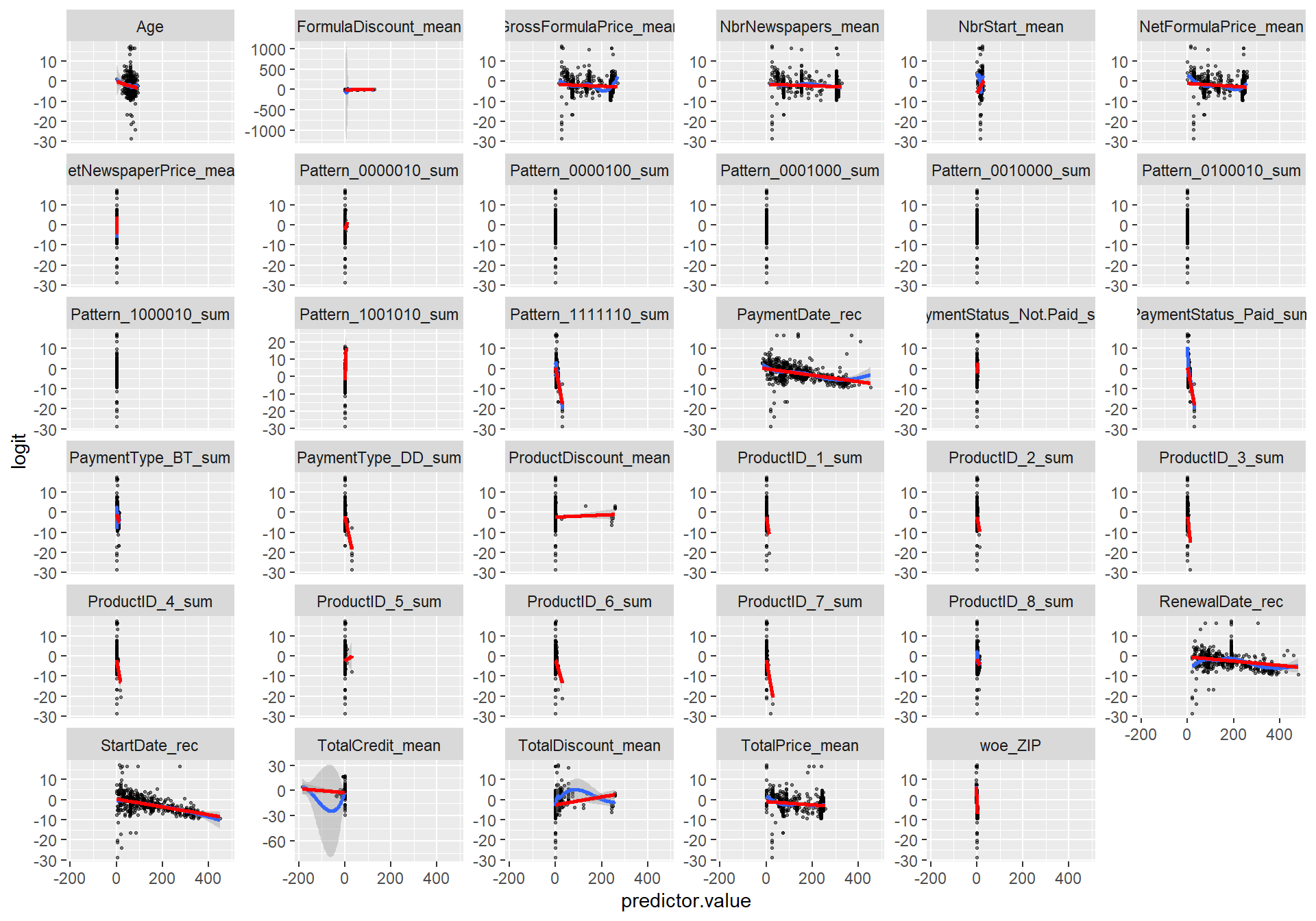
From this plot it is clear that there are some nonlinear effects for several variable. PaymentDate_rec shows a nice nonlinear effect, so we will focus on that one and perform two transformations: a simple power transformation and a Yeo_Johnson transformation.
Polynomials
# Add a polynomial to the power of 2
train_power <- train_final %>%
mutate(TotalDiscount_mean_power = poly(TotalDiscount_mean,
2)) %>%
dplyr::select(!c(CustomerID, TotalDiscount_mean))
model_power <- glm(churn ~ ., train_power, family = binomial)
# Get the fitted terms for plotting Add the lower and
# upperbounds as well
fit_power <- predict(model_power, type = "terms")[, "TotalDiscount_mean_power"]
upperbound <- fit_power + predict(model_power, type = "terms",
se.fit = TRUE)$se.fit[, "TotalDiscount_mean_power"]
lowerbound <- fit_power - predict(model_power, type = "terms",
se.fit = TRUE)$se.fit[, "TotalDiscount_mean_power"]
# Now make the above plot and add the fitted values of our
# model
train_num %>%
filter(predictors == "TotalDiscount_mean") %>%
ggplot(aes(predictor.value, logit)) + geom_point() + geom_smooth(method = "lm") +
geom_line(aes(predictor.value, fit_power), col = "red", size = 1) +
geom_ribbon(aes(ymin = lowerbound, ymax = upperbound, fill = "red"),
linetype = 2, alpha = 0.1, show.legend = FALSE)## `geom_smooth()` using formula 'y ~ x'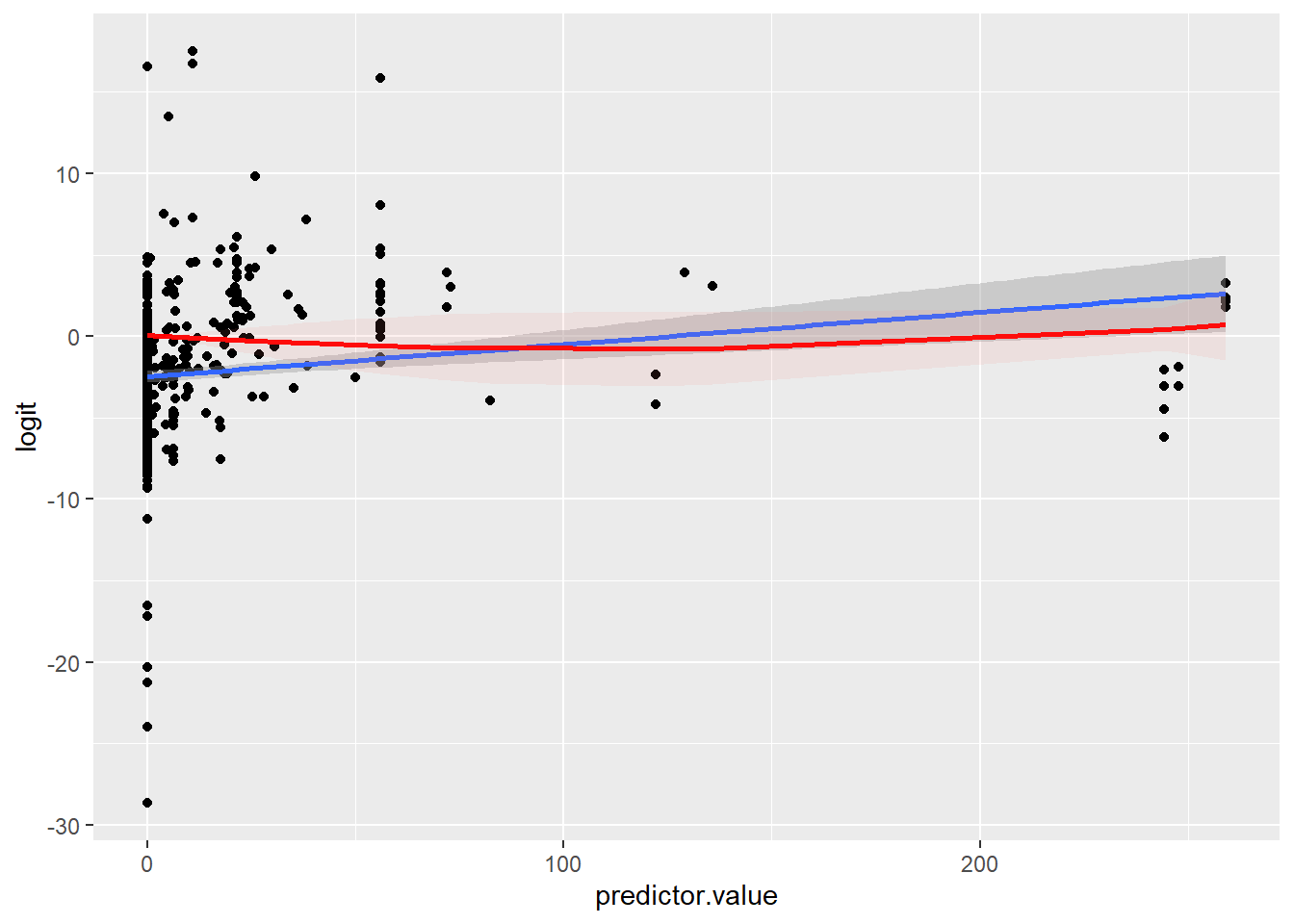
# This does not really fit the data perfectly, so maybe you
# should play around with the degree of the polynomial.Yeo-Johnson
To apply transformations, there are two good packages in R: car (stats driven) and bestNormalize.
The car package allows you to set the lambda parameter yourself, whereas the bestNormalize package automatically finds the optimal lambda = the one that fits best to a normal distribution. For the bestNormalize package, we refer the reader to https://github.com/petersonR/bestNormalize for more information.
p_load(car, bestNormalize)
# The function in the car package is the yjPower function
# ?yjPower Normal values of the YJ transformation range
# between -2 and 2 Apply the YJ function with lambda = 1/2
# again using the TotalDiscount_mean variable
train_yj <- train_final %>%
mutate(TotalDiscount_mean_yj = yjPower(TotalDiscount_mean,
1/2)) %>%
dplyr::select(!c(CustomerID, TotalDiscount_mean))
model_yj <- glm(churn ~ ., train_yj, family = binomial)
# Get the fitted terms for plotting Add the lower and
# upperbounds as well
fit_yj <- predict(model_yj, type = "terms")[, "TotalDiscount_mean_yj"]
upperbound <- fit_yj + predict(model_yj, type = "terms", se.fit = TRUE)$se.fit[,
"TotalDiscount_mean_yj"]
lowerbound <- fit_yj - predict(model_yj, type = "terms", se.fit = TRUE)$se.fit[,
"TotalDiscount_mean_yj"]
# Now make the same plot again and but with the fitted
# values of the YJ function
train_num %>%
filter(predictors == "TotalDiscount_mean") %>%
ggplot(aes(predictor.value, logit)) + geom_point() + geom_smooth(method = "lm") +
geom_line(aes(predictor.value, fit_yj), col = "red", size = 1) +
geom_ribbon(aes(ymin = lowerbound, ymax = upperbound, fill = "red"),
linetype = 2, alpha = 0.1, show.legend = FALSE)## `geom_smooth()` using formula 'y ~ x'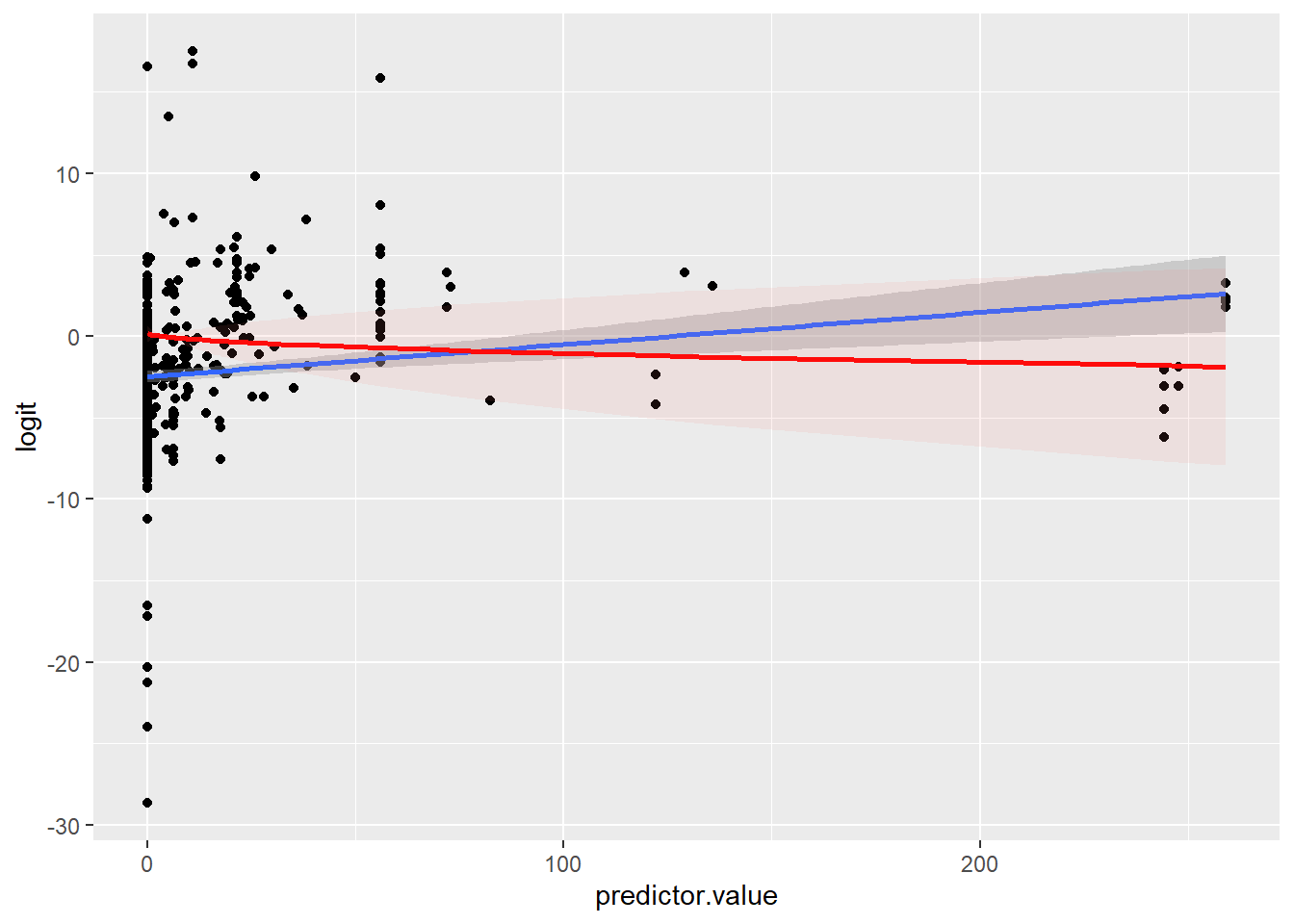
# This value is not really optimal, normally the research
# would experiment with different values of lambda and see
# which one gives the best fit visually or ideally see
# which one gives the best performance on a validation set.
# Question: what is the problem with this visual
# inspection?
# Using the yeojohnson function of the bestNormalize
# package, the optimal lambda value is retrieved
# automatically The best lambda parameters means the one
# that makes it look like a normal distribution Besides the
# Yeo Johnson transformation this package actually tests
# different transformations and informs your which one is
# the best (bestNormalize function) We will set standardize
# to FALSE, since we do not standarize our other
# coefficients. However, a good step before modeling the
# GLM model is to standardize the coefficients
yj <- yeojohnson(train_final$TotalDiscount_mean, standardize = FALSE)
yj## Non-Standardized Yeo-Johnson Transformation with 589 nonmissing obs.:
## Estimated statistics:
## - lambda = -0.9796237
## - mean (before standardization) = 0.2614274
## - sd (before standardization) = 0.4208968# If you want the transformed value, you should predict
# using the YJ object Note that you can also make
# predictions on new data, which makes it fitted for
# predictive settings So re-run all the previous lines of
# code and look at the plot
train_yj <- train_final %>%
mutate(TotalDiscount_mean_yj = predict(yj)) %>%
dplyr::select(!c(CustomerID, TotalDiscount_mean))
model_yj <- glm(churn ~ ., train_yj, family = binomial)
fit_yj <- predict(model_yj, type = "terms")[, "TotalDiscount_mean_yj"]
upperbound <- fit_yj + predict(model_yj, type = "terms", se.fit = TRUE)$se.fit[,
"TotalDiscount_mean_yj"]
lowerbound <- fit_yj - predict(model_yj, type = "terms", se.fit = TRUE)$se.fit[,
"TotalDiscount_mean_yj"]
# Now make the same plot again and but with the fitted
# values of the YJ function
train_num %>%
filter(predictors == "TotalDiscount_mean") %>%
ggplot(aes(predictor.value, logit)) + geom_point() + geom_smooth(method = "lm") +
geom_line(aes(predictor.value, fit_yj), col = "red", size = 1) +
geom_ribbon(aes(ymin = lowerbound, ymax = upperbound, fill = "red"),
linetype = 2, alpha = 0.1, show.legend = FALSE)## `geom_smooth()` using formula 'y ~ x'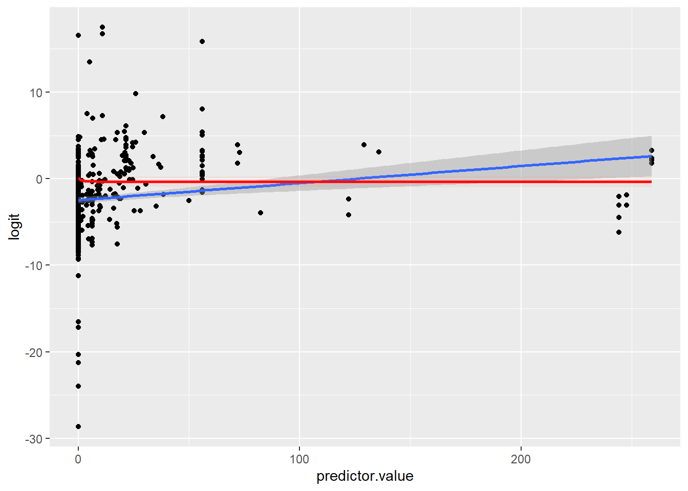
We will not add these transformations to our model add this point in time. However, when using linear models these transformation can significantly increase predictive performance.
Question: why with linear models
2.2.3.2 Standardization and normalization
Often, the variables are standardized or normalized before applying a prediction algorithm. Algorithms that work with distances (e.g., SVM) should always be standardized. Some algorithms benefit from standardizing because it allows you to fairly compare the effect sizes (e.g., linear regression models).Other algorithms need normalization to avoid computational overflow (e.g., neural networks and friends). Tree-based models, on the other hand, do not require scaling and is generally not advisable.
# Standardizing your data can be done like this:
train_sc <- train_final %>%
mutate(across(where(is.numeric), ~scale(.x, center = TRUE,
scale = TRUE)))
train_sc %>%
head()## CustomerID ProductID_1_sum ProductID_2_sum
## 1 497954 -0.1802981 -0.2521697
## 2 855200 -0.1802981 -0.2521697
## 3 870967 -0.1802981 0.8730421
## 4 800576 -0.1802981 -0.2521697
## 5 459730 -0.1802981 -0.2521697
## 6 746052 -0.1802981 -0.2521697
## ProductID_3_sum ProductID_4_sum ProductID_5_sum
## 1 -0.1605461 -0.2437824 -0.1137909
## 2 -0.1605461 -0.2437824 -0.1137909
## 3 -0.1605461 1.2837479 -0.1137909
## 4 -0.1605461 -0.2437824 -0.1137909
## 5 -0.1605461 -0.2437824 -0.1137909
## 6 -0.1605461 -0.2437824 -0.1137909
## ProductID_6_sum ProductID_7_sum ProductID_8_sum
## 1 -0.2998143 -0.1560161 0.5569767
## 2 -0.2998143 -0.1560161 -0.1440046
## 3 -0.2998143 -0.1560161 -0.8449859
## 4 1.1281421 -0.1560161 -0.8449859
## 5 -0.2998143 -0.1560161 0.5569767
## 6 -0.2998143 -0.1560161 0.2064860
## Pattern_0000010_sum Pattern_0000100_sum
## 1 -0.1020741 NaN
## 2 -0.1020741 NaN
## 3 -0.1020741 NaN
## 4 -0.1020741 NaN
## 5 -0.1020741 NaN
## 6 -0.1020741 NaN
## Pattern_0001000_sum Pattern_0010000_sum
## 1 NaN NaN
## 2 NaN NaN
## 3 NaN NaN
## 4 NaN NaN
## 5 NaN NaN
## 6 NaN NaN
## Pattern_0100010_sum Pattern_1000010_sum
## 1 NaN NaN
## 2 NaN NaN
## 3 NaN NaN
## 4 NaN NaN
## 5 NaN NaN
## 6 NaN NaN
## Pattern_1001010_sum Pattern_1111110_sum
## 1 -0.04120428 -0.0525171
## 2 -0.04120428 -0.6048845
## 3 -0.04120428 -0.3287008
## 4 -0.04120428 -0.3287008
## 5 -0.04120428 -0.0525171
## 6 -0.04120428 -0.3287008
## PaymentType_BT_sum PaymentType_DD_sum
## 1 0.09325393 -0.1508845
## 2 -0.72047293 -0.1508845
## 3 -0.31360950 -0.1508845
## 4 -0.31360950 -0.1508845
## 5 0.09325393 -0.1508845
## 6 -0.31360950 -0.1508845
## PaymentStatus_Paid_sum
## 1 -0.03752416
## 2 -0.59706165
## 3 -0.31729291
## 4 -0.31729291
## 5 -0.03752416
## 6 -0.31729291
## PaymentStatus_Not.Paid_sum StartDate_rec
## 1 -0.2976459 -0.8062927
## 2 -0.2976459 -0.6322984
## 3 -0.2976459 2.4234752
## 4 -0.2976459 1.9776150
## 5 -0.2976459 -0.5453013
## 6 -0.2976459 -0.4365549
## RenewalDate_rec PaymentDate_rec
## 1 -0.9990510 -0.7960699
## 2 -0.8883856 -0.9538180
## 3 2.3098439 2.3799251
## 4 1.8561158 2.0539124
## 5 -0.7113210 -0.4069579
## 6 -0.6117221 -0.3017926
## NbrNewspapers_mean NbrStart_mean
## 1 0.83831813 -0.4852796
## 2 -1.71227706 -2.4290956
## 3 0.78432449 -0.0533205
## 4 0.86491202 -0.0533205
## 5 0.77787749 -0.4852796
## 6 -0.04089178 -0.4852796
## GrossFormulaPrice_mean NetFormulaPrice_mean
## 1 0.82232504 0.7910332
## 2 -1.77564500 -1.6067481
## 3 0.69357471 0.7264139
## 4 0.69357471 0.7264139
## 5 0.76196230 0.7910332
## 6 0.02542787 -0.1091142
## NetNewspaperPrice_mean ProductDiscount_mean
## 1 0.12367466 -0.1457419
## 2 1.15892578 -0.1003577
## 3 0.09534996 -0.1457419
## 4 -0.02085542 -0.1457419
## 5 0.20602392 -0.1457419
## 6 -0.30315981 -0.1457419
## FormulaDiscount_mean TotalDiscount_mean
## 1 -0.07517376 -0.1670197
## 2 -0.38100861 -0.2522275
## 3 -0.38100861 -0.2944815
## 4 -0.38100861 -0.2944815
## 5 -0.38100861 -0.2944815
## 6 0.71391155 0.1618449
## TotalPrice_mean TotalCredit_mean Age
## 1 0.855092126 0.1385108 -0.04345565
## 2 -1.502784177 -0.6745143 -0.04345565
## 3 0.793599020 0.1385108 -0.64569980
## 4 0.789755701 0.1037191 -0.44495175
## 5 0.855092126 0.1385108 -0.04345565
## 6 -0.001506848 0.1385108 -0.14382967
## churn RenewalDate_rec_flag PaymentDate_rec_flag
## 1 1 0 0
## 2 1 0 0
## 3 0 0 0
## 4 0 0 0
## 5 1 0 0
## 6 1 0 0
## Gender_flag Gender_F District_1 District_2
## 1 0 0 0 0
## 2 0 1 0 0
## 3 0 0 1 0
## 4 0 1 1 0
## 5 1 0 0 0
## 6 0 0 0 0
## District_4 District_5 District_6 District_7
## 1 0 1 0 0
## 2 0 1 0 0
## 3 0 0 0 0
## 4 0 0 0 0
## 5 0 1 0 0
## 6 0 1 0 0
## District_8 woe_ZIP
## 1 0 -0.251267452
## 2 0 0.005467406
## 3 0 1.360633582
## 4 0 0.385174282
## 5 0 -0.046473335
## 6 0 0.622727107# To scale the test set you should compute the mean and the
# sd of the training set and give these values to the
# center and scale parameters in the scale function
# (Why????)
# Normalizing the data should done like this
min_train <- train_final %>%
select_if(is.numeric) %>%
sapply(., min)
max_train <- train_final %>%
select_if(is.numeric) %>%
sapply(., max)
range_train <- max_train - min_train
train_norm <- data.frame(train_final %>%
select_if(negate(is.numeric)), train_final %>%
select_if(is.numeric) %>%
scale(center = min_train, scale = range_train))
train_norm %>%
head()## CustomerID churn RenewalDate_rec_flag
## 1 497954 1 0
## 2 855200 1 0
## 3 870967 0 0
## 4 800576 0 0
## 5 459730 1 0
## 6 746052 1 0
## PaymentDate_rec_flag Gender_flag Gender_F
## 1 0 0 0
## 2 0 0 1
## 3 0 0 0
## 4 0 0 1
## 5 0 1 0
## 6 0 0 0
## District_1 District_2 District_4 District_5
## 1 0 0 0 1
## 2 0 0 0 1
## 3 1 0 0 0
## 4 1 0 0 0
## 5 0 0 0 1
## 6 0 0 0 1
## District_6 District_7 District_8
## 1 0 0 0
## 2 0 0 0
## 3 0 0 0
## 4 0 0 0
## 5 0 0 0
## 6 0 0 0
## ProductID_1_sum ProductID_2_sum ProductID_3_sum
## 1 0 0.00000000 0
## 2 0 0.00000000 0
## 3 0 0.08333333 0
## 4 0 0.00000000 0
## 5 0 0.00000000 0
## 6 0 0.00000000 0
## ProductID_4_sum ProductID_5_sum ProductID_6_sum
## 1 0.0000000 0 0.0
## 2 0.0000000 0 0.0
## 3 0.1111111 0 0.0
## 4 0.0000000 0 0.1
## 5 0.0000000 0 0.0
## 6 0.0000000 0 0.0
## ProductID_7_sum ProductID_8_sum
## 1 0 0.3333333
## 2 0 0.1666667
## 3 0 0.0000000
## 4 0 0.0000000
## 5 0 0.3333333
## 6 0 0.2500000
## Pattern_0000010_sum Pattern_0000100_sum
## 1 0 NaN
## 2 0 NaN
## 3 0 NaN
## 4 0 NaN
## 5 0 NaN
## 6 0 NaN
## Pattern_0001000_sum Pattern_0010000_sum
## 1 NaN NaN
## 2 NaN NaN
## 3 NaN NaN
## 4 NaN NaN
## 5 NaN NaN
## 6 NaN NaN
## Pattern_0100010_sum Pattern_1000010_sum
## 1 NaN NaN
## 2 NaN NaN
## 3 NaN NaN
## 4 NaN NaN
## 5 NaN NaN
## 6 NaN NaN
## Pattern_1001010_sum Pattern_1111110_sum
## 1 0 0.13333333
## 2 0 0.06666667
## 3 0 0.10000000
## 4 0 0.10000000
## 5 0 0.13333333
## 6 0 0.10000000
## PaymentType_BT_sum PaymentType_DD_sum
## 1 0.3333333 0
## 2 0.1666667 0
## 3 0.2500000 0
## 4 0.2500000 0
## 5 0.3333333 0
## 6 0.2500000 0
## PaymentStatus_Paid_sum
## 1 0.13333333
## 2 0.06666667
## 3 0.10000000
## 4 0.10000000
## 5 0.13333333
## 6 0.10000000
## PaymentStatus_Not.Paid_sum StartDate_rec
## 1 0 0.1361607
## 2 0 0.1718750
## 3 0 0.7991071
## 4 0 0.7075893
## 5 0 0.1897321
## 6 0 0.2120536
## RenewalDate_rec PaymentDate_rec
## 1 0.1561822 0.1804671
## 2 0.1778742 0.1486200
## 3 0.8047722 0.8216561
## 4 0.7158351 0.7558386
## 5 0.2125813 0.2590234
## 6 0.2321041 0.2802548
## NbrNewspapers_mean NbrStart_mean
## 1 0.9406833 0.5294118
## 2 0.1062955 0.2647059
## 3 0.9230201 0.5882353
## 4 0.9493831 0.5882353
## 5 0.9209111 0.5294118
## 6 0.6530634 0.5294118
## GrossFormulaPrice_mean NetFormulaPrice_mean
## 1 0.9148081 0.9382239
## 2 0.1220409 0.1741313
## 3 0.8755201 0.9176319
## 4 0.8755201 0.9176319
## 5 0.8963885 0.9382239
## 6 0.6716360 0.6513771
## NetNewspaperPrice_mean ProductDiscount_mean
## 1 0.7471022 0.00000000
## 2 0.9181674 0.00602529
## 3 0.7424218 0.00000000
## 4 0.7232200 0.00000000
## 5 0.7607096 0.00000000
## 6 0.6765720 0.00000000
## FormulaDiscount_mean TotalDiscount_mean
## 1 0.03649225 0.01817568
## 2 0.00000000 0.00602529
## 3 0.00000000 0.00000000
## 4 0.00000000 0.00000000
## 5 0.00000000 0.00000000
## 6 0.13064599 0.06507079
## TotalPrice_mean TotalCredit_mean Age
## 1 0.9480954 1.0000000 0.6521739
## 2 0.1502126 0.9576721 0.6521739
## 3 0.9272867 1.0000000 0.5869565
## 4 0.9259861 0.9981887 0.6086957
## 5 0.9480954 1.0000000 0.6521739
## 6 0.6582305 1.0000000 0.6413043
## woe_ZIP
## 1 0.5910719
## 2 0.6407753
## 3 0.9031326
## 4 0.7142857
## 5 0.6307196
## 6 0.7602754As you can se from the scaling, some variables get a Nan value, so it would be wise to delete those variables. They will not really add value because their variance is too low.
2.2.3.3 Resampling
Extreme differences in incidence between both classes can be extremely detrimental for your model. When class A (e.g., non-churn) is much more present in your sample than class B (e.g., churn), the model will often simply predict class A as this easy solution may give quite a good performance with regard to accuracy-related measures. So, when unaccounted for, the learners will be biased towards the majority class over the minority class.
So how do we avoid this? By re-sampling your data. You re-sample your data up to a certain degree which will (hopefully) cause your learner to be less biased towards your majority class. This can be a simple 50/50 resampling, where the minority and the majority class are equally present in the resampled sample. But some also suggest to use less extreme forms, where you enhance the relative incidence of the minority class while not reaching the same incidence as the majority class as this is more representative of the ‘actual’ problem than a 50/50 distribution.
Finally, one can both increase the number of minority observations (oversampling) as well as decrease the number of majority observations (undersampling). We will try to give some clarifying examples.
Let’s start with a 50/50 resampling. We will do this on the previously created train_imp data set. The fact that this is only done on the training set is important to notice as resampling of the test set would lead to an unfair evaluation of the algorithm as in reality, you also won’t be deploying it on a 50/50 distributed data set.
# Inspect class imbalance
table(train_imp$churn)##
## 0 1
## 437 152I personally would advise to deploy oversampling here.
Why? Because if we would undersample, we would only keep 304 observations in our training sample (152 churners + 152 non-churners), which is too little to build any decent model (even 589 is already very few).
# Get indices of each group
churners <- which(train_imp$churn == "1")
nonchurners <- which(train_imp$churn == "0")
# See how many instances we would want to have equal number
# as majority_class
n_desired <- length(nonchurners)
resampled_churners <- sample(x = churners, size = n_desired,
replace = TRUE)
print(resampled_churners)## [1] 288 64 586 2 384 416 239 20 340 312 535
## [12] 509 295 41 30 125 383 512 383 296 266 326
## [23] 541 61 471 327 417 2 187 489 336 469 354
## [34] 503 285 540 416 483 129 255 269 219 481 199
## [45] 483 586 389 399 332 399 22 86 199 541 553
## [56] 288 242 390 390 111 197 283 489 200 443 589
## [67] 1 534 6 428 465 199 434 245 54 373 197
## [78] 430 255 443 293 196 509 61 584 297 470 373
## [89] 312 350 504 140 150 286 87 551 568 52 357
## [100] 200 559 559 68 129 383 266 416 385 398 581
## [111] 61 61 326 6 312 139 65 231 412 340 406
## [122] 196 568 259 553 41 503 128 581 242 470 245
## [133] 240 52 144 385 86 398 406 551 85 481 100
## [144] 508 30 150 471 6 496 534 175 340 266 450
## [155] 385 589 389 111 396 574 129 2 144 577 354
## [166] 157 327 68 175 384 242 289 54 111 584 200
## [177] 54 422 151 424 1 111 166 577 354 385 412
## [188] 111 559 504 242 68 531 481 111 200 576 373
## [199] 206 574 503 165 314 43 150 540 584 283 195
## [210] 281 28 242 255 136 584 471 443 412 441 54
## [221] 568 175 385 65 310 219 372 261 286 553 149
## [232] 20 314 296 86 398 398 281 443 28 589 41
## [243] 30 462 568 129 61 297 168 372 41 373 553
## [254] 129 240 54 406 354 231 165 332 297 312 259
## [265] 64 178 196 473 585 242 297 288 295 64 424
## [276] 504 385 465 535 261 553 179 168 196 187 385
## [287] 255 489 87 219 136 288 37 86 584 417 61
## [298] 207 293 5 197 312 568 350 270 215 372 132
## [309] 20 465 270 6 240 540 286 255 296 54 242
## [320] 140 297 496 368 312 61 585 326 259 1 107
## [331] 496 65 24 52 589 128 540 512 168 568 508
## [342] 481 412 354 577 144 52 340 140 149 24 553
## [353] 36 336 149 215 310 100 540 41 68 372 43
## [364] 196 430 336 574 179 489 293 541 441 437 285
## [375] 489 470 390 535 424 68 398 191 542 489 314
## [386] 312 24 255 350 270 504 424 354 44 1 535
## [397] 559 373 266 5 531 384 65 503 503 350 441
## [408] 125 259 245 430 200 471 286 443 508 534 350
## [419] 586 289 399 245 261 551 574 86 366 261 144
## [430] 577 441 175 301 139 297 150 470print(nonchurners)## [1] 3 4 7 9 10 11 12 13 14 15 16
## [12] 17 18 19 21 23 25 26 27 29 31 32
## [23] 33 34 35 38 39 40 42 45 46 47 48
## [34] 49 50 51 53 55 56 57 58 59 60 62
## [45] 63 66 67 69 70 71 72 73 74 75 76
## [56] 77 78 79 80 81 82 83 84 88 89 90
## [67] 91 92 93 94 95 96 97 98 99 101 102
## [78] 103 104 105 106 108 109 110 112 113 114 115
## [89] 116 117 118 119 120 121 122 123 124 126 127
## [100] 130 131 133 134 135 137 138 141 142 143 145
## [111] 146 147 148 152 153 154 155 156 158 159 160
## [122] 161 162 163 164 167 169 170 171 172 173 174
## [133] 176 177 180 181 182 183 184 185 186 188 189
## [144] 190 192 193 194 198 201 202 203 204 205 208
## [155] 209 210 211 212 213 214 216 217 218 220 221
## [166] 222 223 224 225 226 227 228 229 230 232 233
## [177] 234 235 236 237 238 241 243 244 246 247 248
## [188] 249 250 251 252 253 254 256 257 258 260 262
## [199] 263 264 265 267 268 271 272 273 274 275 276
## [210] 277 278 279 280 282 284 287 290 292 294 298
## [221] 299 300 302 303 304 305 306 307 308 309 311
## [232] 313 315 316 317 318 319 320 321 322 323 324
## [243] 325 328 329 330 331 333 334 335 337 338 339
## [254] 341 342 343 344 345 346 347 348 349 351 352
## [265] 353 355 356 358 359 360 361 362 363 364 365
## [276] 367 369 370 371 374 375 376 377 378 379 380
## [287] 382 386 387 388 391 392 393 394 395 397 400
## [298] 401 402 403 404 405 407 408 409 410 411 413
## [309] 414 415 418 419 420 421 423 426 427 429 431
## [320] 432 433 435 436 438 439 440 442 445 446 447
## [331] 448 449 451 452 453 454 455 456 457 458 460
## [342] 461 463 464 466 467 468 472 474 475 476 477
## [353] 478 479 480 482 484 485 486 487 488 490 491
## [364] 492 493 494 495 497 498 499 500 501 502 505
## [375] 506 507 510 511 513 514 515 516 517 518 519
## [386] 520 521 522 523 524 525 526 527 528 529 530
## [397] 532 533 536 537 538 539 543 544 545 546 547
## [408] 548 549 550 552 554 555 556 557 558 560 561
## [419] 562 563 564 565 566 567 569 570 571 572 573
## [430] 575 578 579 580 582 583 587 588# Combine into one large data set
oversampled_train <- train_imp[c(resampled_churners, nonchurners),
]
table(oversampled_train$churn)##
## 0 1
## 437 437# How would our sample look like if we undersampled the
# minority class? Get indices of each group
churners <- which(train_imp$churn == "1")
nonchurners <- which(train_imp$churn == "0")
# See how many instances we would want to have equal number
# as majority_class
n_desired <- length(churners)
resampled_nonchurners <- sample(x = nonchurners, size = n_desired,
replace = FALSE)
undersampled_train <- train_imp[c(resampled_nonchurners, churners),
]
table(undersampled_train$churn)##
## 0 1
## 152 152What if we want to resample to another ratio? Well, this is relatively quickly adapted into our code. Take, for example, the 1/2 ratio (double as much non-churners in the final set).
churners <- which(train_imp$churn == "1")
nonchurners <- which(train_imp$churn == "0")
# See how many instances we would want to have equal number
# as majority_class
n_desired <- length(nonchurners)/2
resampled_churners <- sample(x = churners, size = n_desired,
replace = TRUE)
oversampled_train2 <- train_imp[c(resampled_churners, nonchurners),
]
table(oversampled_train2$churn)##
## 0 1
## 437 218While this is fairly easy to implement yourselves, several packages exist that do this automatically. A package that I would highly recommend you to use, is the unbalanced package. This does not only include over- and undersampling, but also more advanced techniques, such as SMOTE.
The most important function is the ubBalance function. The function requires the independent and dependent variables to be feeded independently from each other. The type argument specifies which kind of resampling you want to use (e.g., oversampling, SMOTE, …). The positive argument identifies which factor level is the minority class (error in documentation states majority)
p_load(unbalanced)
# Always check out documentation ?ubBalance
input <- train_imp
output <- input$churn
input$churn <- NULL
# Undersampling
result <- ubBalance(X = input, Y = output, positive = "1", type = "ubUnder",
perc = 50)
undersample_package <- cbind(result$X, result$Y)
table(undersample_package$`result$Y`)##
## 0 1
## 152 152Will this undersample_package dataset be the exact same as the undersampled_train dataset? Why (not)?
# Oversampling
# If K=0: sample with replacement from the minority class
# until we have the same number of instances in each class.
# If K>0: sample with replacement from the minority class
# until we have k-times the original number of minority
# instances.
result <- ubBalance(X = input, Y = output, positive = "1", type = "ubOver",
k = 0)
oversample_package <- cbind(result$X, result$Y)
table(oversample_package$`result$Y`)##
## 0 1
## 437 437# SMOTE
# Check ?ubSMOTE
# SMOTE can't handle char input ==> transform
input <- input %>%
mutate_if(is.character, as.factor)
result <- ubBalance(X = input, Y = output, positive = "1", type = "ubSMOTE",
percUnder = 120, percOver = 500)
smote <- cbind(result$X, result$Y)
table(smote$`result$Y`)##
## 0 1
## 912 9122.2.3.4 Variable selection
We will not scale the data to perform feature selection. Whether you should or should not perform scaling before variable selection is debatable and depends on your data and the applications. In the end there is nothing wrong with performing scaling and some algorithms (cf. supra) might even benefit from it.
As an exercise, you can use the scaled data and check whether the results change.
Filter methods
Since we are have categorical response we will use the fisher score for the continuous variables and the information value for the categorical variables.
The fisher score can be calculate with the do.fscore function of the Rdimtools package. This package contains a lot of dimensionality reduction and feature extraction methods. See https://github.com/kyoustat/Rdimtools for more information.
p_load(Rdimtools)
# Of course this can only be done on the continuous
# variables ndim select the top X dimensions in terms of
# Fisher score In CCP literature the top 20 variables are
# often selected as a first filter
fscore <- do.fscore(X = train_final %>%
select_if(is.numeric) %>%
as.matrix(), label = train_final$churn, ndim = 20)
# Which variables are selected?
(varsel_fisher <- names(train_final %>%
select_if(is.numeric))[fscore$featidx])## [1] "woe_ZIP"
## [2] "StartDate_rec"
## [3] "PaymentDate_rec"
## [4] "FormulaDiscount_mean"
## [5] "NetNewspaperPrice_mean"
## [6] "TotalPrice_mean"
## [7] "PaymentStatus_Paid_sum"
## [8] "Pattern_1111110_sum"
## [9] "NetFormulaPrice_mean"
## [10] "PaymentType_BT_sum"
## [11] "NbrStart_mean"
## [12] "ProductID_8_sum"
## [13] "RenewalDate_rec"
## [14] "NbrNewspapers_mean"
## [15] "GrossFormulaPrice_mean"
## [16] "TotalDiscount_mean"
## [17] "PaymentStatus_Not.Paid_sum"
## [18] "PaymentType_DD_sum"
## [19] "Pattern_1001010_sum"
## [20] "ProductID_6_sum"# Question: The selection of woe_ZIP is actually pretty
# trivial, why?
# For the categorical variables, we can use the woe
# function of the klaR package Since this function also
# calculates the IV, we can also use it as a filter method
# Make sure that everything is a factor for this function
train_final <- train_final %>%
mutate_if(negate(is.numeric), as.factor)
(woes <- klaR::woe(churn ~ ., data = train_final %>%
select_if(negate(is.numeric)) %>%
dplyr::select(!c(CustomerID)), zeroadj = 0.05))## At least one empty cell (class x level) does exists. Zero adjustment applied!
## At least one empty cell (class x level) does exists. Zero adjustment applied!
## At least one empty cell (class x level) does exists. Zero adjustment applied!
## At least one empty cell (class x level) does exists. Zero adjustment applied!## Information values of transformed variables:
##
## IV
## RenewalDate_rec_flag 0.961485687
## District_7 0.121524361
## PaymentDate_rec_flag 0.101454512
## Gender_flag 0.100879141
## District_5 0.087944494
## District_6 0.062063245
## Gender_F 0.017131993
## District_1 0.012652996
## District_4 0.003805273
## District_8 0.003805273
## District_2 0.002972176# Now just select the variables with an IV>0.10
(varsel_iv <- names(train_final %>%
select_if(negate(is.numeric)) %>%
dplyr::select(!c(CustomerID, churn)))[which(woes$IV > 0.1)])## [1] "RenewalDate_rec_flag" "PaymentDate_rec_flag"
## [3] "Gender_flag" "District_7"# Note that in the value representation phase you can also
# bin the categorical or continuous variables based on the
# IV, which also leads to a form of feature selection It is
# also possible to calculate the IVs on continuous
# variables. In that case you can use the woeBinning
# package and see what the IVs are of each optimal
# woeBinning continuous variable
# To summarize, using the filter methods, we would select
# the following variables
(varsel_filter <- c(varsel_fisher, varsel_iv))## [1] "woe_ZIP"
## [2] "StartDate_rec"
## [3] "PaymentDate_rec"
## [4] "FormulaDiscount_mean"
## [5] "NetNewspaperPrice_mean"
## [6] "TotalPrice_mean"
## [7] "PaymentStatus_Paid_sum"
## [8] "Pattern_1111110_sum"
## [9] "NetFormulaPrice_mean"
## [10] "PaymentType_BT_sum"
## [11] "NbrStart_mean"
## [12] "ProductID_8_sum"
## [13] "RenewalDate_rec"
## [14] "NbrNewspapers_mean"
## [15] "GrossFormulaPrice_mean"
## [16] "TotalDiscount_mean"
## [17] "PaymentStatus_Not.Paid_sum"
## [18] "PaymentType_DD_sum"
## [19] "Pattern_1001010_sum"
## [20] "ProductID_6_sum"
## [21] "RenewalDate_rec_flag"
## [22] "PaymentDate_rec_flag"
## [23] "Gender_flag"
## [24] "District_7"# which is a reduction of the number of variables
((ncol(train_final) - 1) - length(varsel_filter))/(ncol(train_final) -
1)## [1] 0.4893617Wrapper methods
One downside of the above methods is that they are not based on any performance measure, nor do they use a prediction model to come up with the predictive value of features. As a result, you could ask yourself the question: are these filter methods really selecting the most predictive features? One famous wrapper methods is stepwise variable selection. However, stepwise variable selection has several downsides and will not be covered here. We cover it when discussing linear/logistic regression, but be advised that feature selection baed on stepwise regression is often faulty. A better way is to use regularization, which will also be covered later when discussing logistic regression.
Here, we will discuss recursive feature elimination based on random forest, due to its immense popularity in industry (and academic literature). As mentioned in the slides, the two most important packages are: varSelRF and Boruta.
p_load(varSelRF, Boruta)
# varSelRF ?varSelRF vars.drop.frac = 0.20, the fraction of
# variables dropped in each iteration, the higher this
# number, the more aggressive the feature selection Can be
# compared to a learning rate parameter in neural nets
# ntree = the number of trees in the first forest (like in
# randomForest) ntreeIterat = the number of trees to use in
# the subsequent forests It has been shown that more
# iterations do not lead to a better performance
rf_vsrf <- varSelRF(train_final[, !names(train_final) %in% c("churn",
"CustomerID")], train_final$churn, vars.drop.frac = 0.2,
ntree = 500, ntreeIterat = 100)
(varsel_vsrf <- rf_vsrf$selected.vars)## [1] "NetFormulaPrice_mean" "PaymentDate_rec"
## [3] "RenewalDate_rec" "StartDate_rec"
## [5] "woe_ZIP"# As an exercise you can play around with the parameters
# and see what happens
# Boruta ?Boruta doTrace = 0 means no tracing, 1 means
# reporting decision about each attribute as soon as it is
# justified, 2 means the same as 1, plus reporting each
# importance source run, 3 means the same as 2, plus
# reporting of hits assigned to yet undecided attributes.
(rf_boruta <- Boruta(train_final[, !names(train_final) %in% c("churn",
"CustomerID")], train_final$churn, doTrace = 0))## Boruta performed 99 iterations in 38.28913 secs.
## 18 attributes confirmed important:
## FormulaDiscount_mean,
## GrossFormulaPrice_mean, NbrNewspapers_mean,
## NbrStart_mean, NetFormulaPrice_mean and 13
## more;
## 26 attributes confirmed unimportant:
## District_1, District_2, District_4,
## District_5, District_6 and 21 more;
## 2 tentative attributes left: Age,
## ProductDiscount_mean;# Algorithm stops when only Confirmed attributes are left,
# or when it reaches maxRuns importance source runs. If
# the second scenario occurs, some attributes may be left
# without a decision. They are claimed Tentative. You may
# try to extend maxRuns or lower pValue to clarify them,
# but in some cases their importances do fluctuate too much
# for Boruta to converge
# Another fix can be to use the TentativeRoughFix function,
# which performs a weaker significance test
# To get a nice overview of the important and signficant
# variables, you can make a plot
# green = confirmed, yellow = tentative, red = rejected,
# blue = shadow
plot(rf_boruta)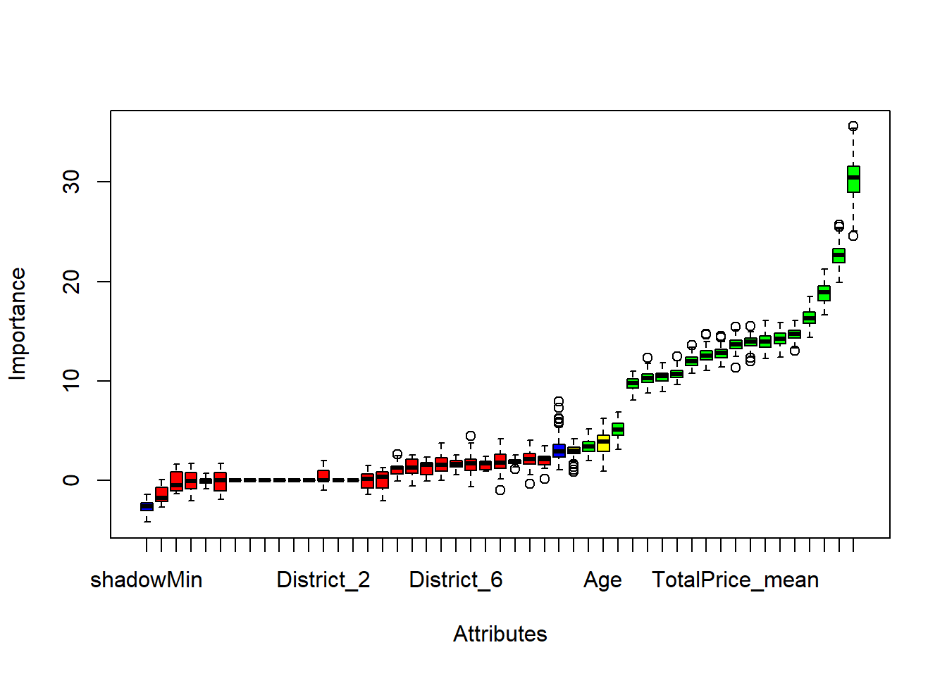
# Let's just select the confirmed variables As an exercise,
# you can try the rough fix or increase the maxRuns or the
# significance level and see what happens
(varsel_boruta <- names(rf_boruta$finalDecision[rf_boruta$finalDecision ==
"Confirmed"]))## [1] "ProductID_8_sum"
## [2] "Pattern_1111110_sum"
## [3] "PaymentType_BT_sum"
## [4] "PaymentType_DD_sum"
## [5] "PaymentStatus_Paid_sum"
## [6] "StartDate_rec"
## [7] "RenewalDate_rec"
## [8] "PaymentDate_rec"
## [9] "NbrNewspapers_mean"
## [10] "NbrStart_mean"
## [11] "GrossFormulaPrice_mean"
## [12] "NetFormulaPrice_mean"
## [13] "NetNewspaperPrice_mean"
## [14] "FormulaDiscount_mean"
## [15] "TotalDiscount_mean"
## [16] "TotalPrice_mean"
## [17] "RenewalDate_rec_flag"
## [18] "woe_ZIP"