5 Ensembles
This chapter will cover the concepts seen in Ensembles. We will discuss more in detail how to implement advanced ensemble models. Make sure that you go over the video and slides before going over this chapter.
5.1 Bagging
Up until now we have seen single classifiers. Those algorithms all try to match a pre-specified model structure to the relationship between predictors and response. This results in several model-specific issues: a regression model never learns complex nonlinear relations, and a decision tree will never know how to estimate the impact of an increase beyond the observed training range (as no splits can be made there, notice the difference with the ever-inclining regression slopes). To overcome this, people thought about combining several single classifiers. Such a combination of single classifiers is called an ensemble.
While you can build any combination of single classifiers by use of a certain aggregation rule (e.g., performance-weighted predictions), several popular pre-configured ensembles exist. A popular building block for ensembles are decision trees. This is because decision trees tend to overfit heavy to the data and are unstable. This means that small deviations in the training data are enough to deliver very different decision trees (a small deviation in the top node split will heavily impact the rest of the tree’s structure). This knowledge is used in bagged decision trees. Bagging is short for bootstrap aggregation and a bootstrap sample is nothing different than a sample with replacement.
As you take different samples for each tree, small deviations occur in the training set. These small deviations cause the trees to become relatively different. Only the tree structures that are present in most trees will be representive of the true underlying relationship (without overfitting)! By aggregating (averaging) all the predictions, you have predictions which incorporate the aspects of each unique tree. Aspects that are present in each tree will weigh more heavy in the overall predictions.
Now let us put this to practice ourselves. We will be using again the data from our NPC.
# Temporarily turn warnings off (many informative are
# thrown during various iterations of some ensembles)
defaultW <- getOption("warn")
options(warn = -1)

# Read in the data
load("C:\\Users\\matbogae\\OneDrive - UGent\\PPA22\\PredictiveAnalytics\\Book_2022\\data codeBook_2022\\TrainValTest.Rdata")
We will compare how a single decision tree performs on this data compared to bagged approach, where we use 100 bags.
set.seed(123)

if (!require("pacman")) install.packages("pacman")
## Loading required package: pacmanrequire("pacman", character.only = TRUE, quietly = TRUE)
p_load(AUC, rpart, tidyverse)
# Create one tree:
tree <- rpart(yTRAINbig ~ ., BasetableTRAINbig)
predTREE <- predict(tree, BasetableTEST)[, 2]
AUC::auc(AUC::roc(predTREE, yTEST))## [1] 0.8920165The single decision tree does fairly well. But now how do we construct bagged trees? First, we start by creating 100 bootstrap samples, and we fit a decision tree on each sample. Next, once these 100 decision trees are fit, you use each of them to create predictions on the validation set. All predictions are then stored in the baggedpredictions object. We take the average value of all these predicted probabilities to have a final estimate (finalprediction).
We observe an enormous increase in predictive performance! This is also still observed when we deploy the methodology to have a final performance estimate.
ensemblesize <- 100
ensembleoftrees <- vector(mode = "list", length = ensemblesize)

# Fit the ensemble
for (i in 1:ensemblesize) {
    bootstrapsampleindicators <- sample.int(n = nrow(BasetableTRAINbig),
        size = nrow(BasetableTRAINbig), replace = TRUE)
    ensembleoftrees[[i]] <- rpart(yTRAINbig[bootstrapsampleindicators] ~
        ., BasetableTRAINbig[bootstrapsampleindicators, ])
}

# Make predictions
baggedpredictions <- data.frame(matrix(NA, ncol = ensemblesize,
    nrow = nrow(BasetableTEST)))

for (i in 1:ensemblesize) {
    baggedpredictions[, i] <- as.numeric(predict(ensembleoftrees[[i]],
        BasetableTEST)[, 2])
}

finalprediction <- rowMeans(baggedpredictions)

# Evaluate
AUC::auc(AUC::roc(finalprediction, yTEST))
## [1] 0.9564843Note that there are packages in R to that build a bagging for you. Good packages are: adabag and ipred.
5.2 Random Forest
While bagging already brings enormous improvement over regular decision trees, this only alters the input observations but leaves the predictors untouched. As such the reduction in variance can be limited if there are only a few important variables. Breiman reasoned that there should also be more ariation induced in the model construction and that the trees should be decorrelated. He combined bootstrap aggregating with a random subset of variables as possible candidates at each split. This brings great variation in each tree, as the most obvious splitting criterion may not always be a possible candidate, which pushes the tree to finding other structures to fit to the observed pattern.
We use the randomForest package, which automatically creates a random forest, so do not worry about implementing these random splitting candidates yourself. This package was actually written by one of the PhD students of Leo Breiman in Fortran.
p_load(randomForest)

# create a first random forest model
rFmodel <- randomForest(x = BasetableTRAINbig, y = yTRAINbig,
    ntree = 500, importance = TRUE)

predrF <- predict(rFmodel, BasetableTEST, type = "prob")[, 2]

# assess final performance
AUC::auc(AUC::roc(predrF, yTEST))
## [1] 0.9658171During session 2, we saw how to optimize the number of trees, but in reality this is often skipped as the number of trees is rather robust, as long as you set it high enough (Breiman recommends 500 or 1000). Let’s see what happens if we would tune the number of trees.
rFmodel <- randomForest(x = BasetableTRAIN, y = yTRAIN, xtest = BasetableVAL,
    ytest = yVAL, ntree = 1000, importance = TRUE)

# Make a plot red dashed line: class error 0 green dotted
# line: class error 1 black solid line: OOB error we see
# that class 0 has lower error than class 1. This is
# because there are much more zeroes to learn from.
head(plot(rFmodel))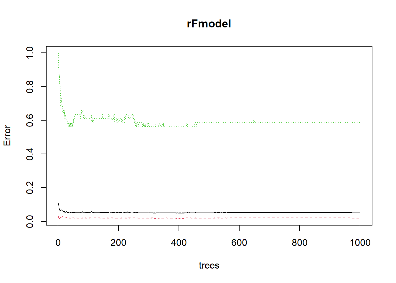
##             OOB          0         1
## [1,] 0.10588235 0.02145923 1.0000000
## [2,] 0.09501188 0.03307888 0.9642857
## [3,] 0.07824427 0.02448980 0.8529412
## [4,] 0.07512521 0.02495544 0.8157895
## [5,] 0.06864275 0.01661130 0.8717949
## [6,] 0.06616541 0.01760000 0.8250000
We already observe a very flat out-of-bag error.However, when we select the optimal number of trees according to this plot, we see that performance is much lower than when we did not optimize for the value. Just set you number of trees large enough. By the way, it is exactly this performant, robust behaviour which makes random forest such a popular algorithm. Almost all modelers add a random forest model to compare their performance with.
Note that random forest can be sensitive to the mtry parameter, or the number of random variables to select at each split. You can try for yourself what optimizing the mtry would do.
# create the model with the optimal ensemble size
rFmodel <- randomForest(x = BasetableTRAINbig, y = yTRAINbig,
    ntree = which.min(rFmodel$test$err.rate[, 1]), importance = TRUE)
predrF <- predict(rFmodel, BasetableTEST, type = "prob")[, 2]
# Final performance
AUC::auc(AUC::roc(predrF, yTEST))
## [1] 0.9401424We will be saving this model to use in a later session. As you might have noticed, while we are getting strong predictive performances, we have yet to get insights into these models, which is much harder for these complex models.
save(rFmodel, file = "randomForestSession4.Rdata")Another excellent packages for random forest is ranger, which is written in C++ and is blazingly fast (https://github.com/imbs-hl/ranger). Besides the speed of execution, the package also contains an implementation of extremely randomized trees. The ranger has actually become the default random forest implementation and is used in several major packages (e.g., Boruta).
# RANGER RF
p_load(ranger)

# Model
rangerModel <- ranger(x=BasetableTRAINbig,
                      y= yTRAINbig,
                      num.trees=500, #by default 500
                      importance = 'permutation', #to get measure of variable importance
                      probability = TRUE) #to get probability estimates

# Predict
predranger <- predict(rangerModel,
                  BasetableTEST)$predictions[,2]

# Evaluation
AUC::auc(roc(predranger ,yTEST))
## [1] 0.9715142#XTREES
Xtree_model <- ranger(x=BasetableTRAINbig,
y=yTRAINbig,
num.trees=500, #by default 500
splitrule = 'extratrees', #to model xtrees
probability = TRUE) #to get probability estimates
# Predict
predXtree <- predict(Xtree_model,
BasetableTEST)$predictions[,2]
# Evaluation
AUC::auc(roc(predXtree ,yTEST))## [1] 0.9709525.3 Boosting
Both bagging and random forest are parallel ensemble techniques. This means that each single classifier is built independent from the other single classifiers. This has the advantage that you can create many classifier simultaneously, but the disadvantage that all these classifiers do not learn from each other.
In sequential ensembles, the single classifiers do learn from each other. Consider the case where it is very hard to predict churn behaviour of an elder, very loyal customer. Parallel ensembles would continue on making the same mistakes, while sequential ensembles would give special attention to these hard-to-classify instances. They boost performance by give additional weight to these instances in the optimized loss function. Hence the name boosting.
Several boosting algorithms exist. We will cover four popular ones: adaptive boosting (AdaBoost), extreme gradient boosting (XGBoost), catboost and LightGBM.
5.3.1 Adaboost
AdaBoost adds data-induced diversity by taking bootstrap samples for each iteration. A model is then fitted on the sample, but the weights (need to be initialized) are based on the misclassification costs of the previous iteration! This of course makes the number of iterations highly linked to overfitting: the more you learn hard-to-classify instances, the more likely you will be learning instance-dependent patterns rather than generalizable patterns. Therefore, the most important parameter is the number of iterations, which needs to be optimized. We will be using the fastAdaboost package, which has an implementation of the AdaBoost algorithms using decision trees as single classifiers. Note that to safe time, we only try a couple of options for niter options. In reality, you perform a more extensive grid search (e.g., seq(10,200,10)).
p_load(fastAdaboost)
aucs_train <- vector()
aucs_val <- vector()

# fastADaboost uses the formula notation, so make the data
# compatible
train_ada <- BasetableTRAIN
train_ada$y <- yTRAIN

trainbig_ada <- BasetableTRAINbig
trainbig_ada$y <- yTRAINbig

val_ada <- BasetableVAL
val_ada$y <- yVAL

test_ada <- BasetableTEST
test_ada$y <- yTEST

# start the loop
iters <- c(1, 10, 50, 100, 200)
j <- 0
for (iter in iters) {
    j <- j + 1
    ABmodel <- adaboost(y ~ ., train_ada, nIter = iter)

    predAB <- predict(ABmodel, BasetableTRAIN)$prob[, 2]
    aucs_train[j] <- AUC::auc(AUC::roc(predAB, yTRAIN))

    predAB <- predict(ABmodel, BasetableVAL)$prob[, 2]
    aucs_val[j] <- AUC::auc(AUC::roc(predAB, yVAL))
}

plot(iters, aucs_train, type = "l", col = "green")
lines(iters, aucs_val, col = "red")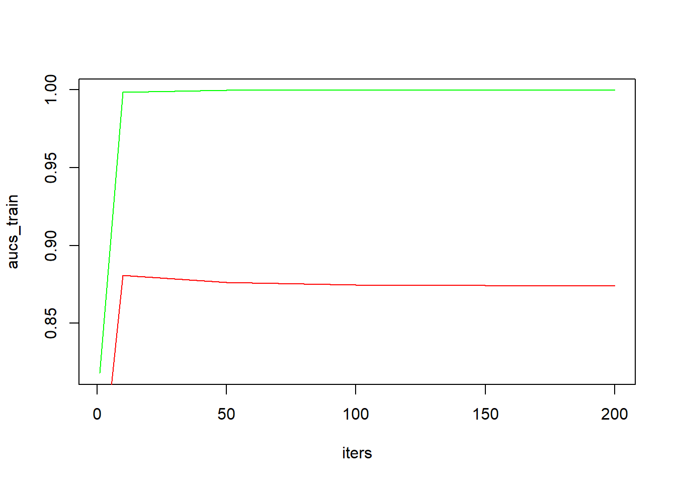
(niter_opt <- iters[which.max(aucs_val)])## [1] 10Already after relatively few iterations (10), we observe the validation AUC to have reached its maximum. Continued fitting on the training set leads to a perfect fit on the training data (AUCtrain = 1; green line), but this actually slightly decreases the performance on the validation set. Better performance would be obtained when we would have stopped learning after 10 iterations.
ABmodel <- adaboost(y ~ ., trainbig_ada, nIter = niter_opt)
predAB <- predict(ABmodel, BasetableTEST)$prob[, 2]
AUC::auc(AUC::roc(predAB, yTEST))
## [1] 0.9434975.3.2 XGBoost
Researchers were attracted to the sequential learning idea behind adaboost. This caused them to come up with gradient boosting. Gradient boosting is a generalization of adaboost. While AdaBoost is a special case with a particular loss function, gradient boosting can be regarded as an ‘overall’ solution to building sequential learners. Rather than simply weighting instances based on the misclassification costs, other step sizes are possible. More importantly, since gradient boosting can be solved by using gradient descent, it can optimize different loss functions. This causes both the step size of the gradient descent algorithm and the used loss function to be important paramaters. The original gradient boosting algorithm is implemented in the gbm package, however nowadays another boosting variant has taken over, namely XGBoost.
XGBoost algorithm is an improved implementation of the gradient boosting algorithm. The algorithm is computationally more efficient due to the inclusion of the second order derivative in its search strategy, but also less prone to overfitting due to the addition of a regularization term (similar to regression, or cost-complexity in decision trees). The combination of both resulted in the algorithm being very performant both in terms in predictive power as well as computational efficiency. This made the algorithm’s popularity heavily peak in recent years.
Just like keras (see Session 5), XGBoost is actually based on C++ code and the R-functions are just wrapper functions around the original code (actually the same is done in Python, so XGBoost has the same functionalities in both R and Python). As a results XGBoost only works with numeric vectors. This means we once again have to change the data type we are feeding to the algorithm. We will be optimizing for multiple parameters at once:
- The number of boosting rounds (
nround), as this is an important parameter for all boosting algorithms. - The parameter
eta(learning rate) determines the step size during each improvement, -Gammaon its term determines the regularization importance.
Another important parameter is the depth of the trees, since this can also control for overfitting and underfitting. However, by using the regularization term this option becomes less important.
p_load(xgboost)

# preparing matrices again notice that the factor should be
# set as numeric (why????)
dtrain <- xgb.DMatrix(data = as.matrix(BasetableTRAIN), label = as.numeric(as.character(yTRAIN)))
dtrainbig <- xgb.DMatrix(data = as.matrix(BasetableTRAINbig),
    label = as.numeric(as.character(yTRAINbig)))
dval <- xgb.DMatrix(data = as.matrix(BasetableVAL), label = as.numeric(as.character(yVAL)))
dtest <- xgb.DMatrix(data = as.matrix(BasetableTEST), label = as.numeric(as.character(yTEST)))

# Set the hyperparameters
eta <- c(0.01, 0.1, 0.2, 0.5)
nround <- c(2, 5, 10, 20, 50, 100, 200)
gamma <- c(0.5, 1, 1.5, 2)

# create data frame of all possible combinations
params <- expand.grid(eta, nround, gamma)
colnames(params) <- c("eta", "nround", "gamma")
head(params, 20)
## eta nround gamma
## 1 0.01 2 0.5
## 2 0.10 2 0.5
## 3 0.20 2 0.5
## 4 0.50 2 0.5
## 5 0.01 5 0.5
## 6 0.10 5 0.5
## 7 0.20 5 0.5
## 8 0.50 5 0.5
## 9 0.01 10 0.5
## 10 0.10 10 0.5
## 11 0.20 10 0.5
## 12 0.50 10 0.5
## 13 0.01 20 0.5
## 14 0.10 20 0.5
## 15 0.20 20 0.5
## 16 0.50 20 0.5
## 17 0.01 50 0.5
## 18 0.10 50 0.5
## 19 0.20 50 0.5
## 20 0.50 50 0.5We will validate which parameter setting in the grid leads to the most performant model. The option objective = "binary:logistic" tells the xgboost algorithm to use a logit activation function (and hence output probabilities). Otherwise it would assume it was handling a regression.
aucs_xgb <- vector()
for (row in 1:nrow(params)) {
    par <- params[row, ]
    xgb <- xgb.train(data = dtrain, eta = par$eta, nrounds = par$nround,
        gamma = par$gamma, objective = "binary:logistic", verbose = 0)
    pred <- predict(xgb, dval)  # automatically knows to only use predictor variables
    aucs_xgb[row] <- AUC::auc(AUC::roc(pred, yVAL))
}

(optimal_params <- params[which.max(aucs_xgb), ])
## eta nround gamma
## 40 0.5 10 1# Build the final
xgb <- xgb.train(data = dtrainbig, eta = optimal_params$eta,
nrounds = optimal_params$nround, gamma = optimal_params$gamma,
objective = "binary:logistic", verbose = 0)
pred <- predict(xgb, dtest)
AUC::auc(AUC::roc(pred, yTEST))## [1] 0.9611319XGBoost is, together with the random forest model(s) the first to score above AUC = 0.96. As the algorithm is quite sensitive towards its parameter settings, it might well be that a more condensed grid around the current optimal values even leads to a better performance. The good performance of XGBoost is not surprising as this is often the winner in a lot of Kaggle competitions. In a lot of business applications, you will actually see that XGBoost is one of the top performers (even outperforming full-blown deep neural networks, as we will see in the next chapter).
We will also be saving this model to use in a later session.
save(xgb, file = "XGBSession4.Rdata")5.3.3 LightGBM
LightGBM is a memory-efficient and highly scalable gradient boosting alternative. The main problems that LightGBM tackles to increase the computation speed are decreasing the number of features and inputs to calculate the gradient. Moreover, LightGBM also proposes a histogram-based leaf-wise tree building procedure that further increases computational speed. LightGBM is designed by Microsoft and therefore often used in production with for example Microsoft Azure. Let’s check how it compares to XGBoost.
# LIGHTGBM
p_load(lightgbm)

# Model One advantage of lightgbm is that it normally
# accepts a matrix from R However, the data should again be
# numeric (also the label) Set parameter grid For a full
# list see:
# https://lightgbm.readthedocs.io/en/latest/Parameters.html
leaves <- c(2, 4, 6, 8)
nround <- c(2, 5, 10, 20, 50, 100, 200)
learning_rate <- c(0.01, 0.05, 0.1, 0.2, 0.5)

# create data frame of all possible combinations
params <- expand.grid(leaves, nround, learning_rate)
colnames(params) <- c("leaves", "nround", "learning_rate")

aucs <- vector()
for (row in 1:nrow(params)) {
    # set parameters
    par <- params[row, ]
    param_set <- list(num_leaves = par[, "leaves"], learning_rate = par[,
        "learning_rate"], objective = "binary", boosting = "gbdt",
        num_iterations = par[, "nround"])
    # model
    lgbm_model <- lightgbm(data = as.matrix(BasetableTRAIN),
        params = param_set, label = as.numeric(as.character(yTRAIN)),
        verbose = -1)

    # predict
    pred <- predict(lgbm_model, as.matrix(BasetableVAL))

    # evaluate
    aucs[row] <- AUC::auc(AUC::roc(pred, yVAL))
}

(optimal_paramsLGBM <- params[which.max(aucs), ])
## leaves nround learning_rate
## 98 4 20 0.2# Build the final model on the optimal parameters
final_param_set <- list(num_leaves = optimal_paramsLGBM[, "leaves"],
learning_rate = optimal_paramsLGBM[, "learning_rate"], objective = "binary",
boosting = "gbdt", num_iterations = optimal_paramsLGBM[,
"nround"])
lgbm_model <- lightgbm(data = as.matrix(BasetableTRAINbig), params = final_param_set,
label = as.numeric(as.character(yTRAINbig)), verbose = -1)
# Predict
predlgbm <- predict(lgbm_model, as.matrix(BasetableTEST))
# Evaluate
AUC::auc(AUC::roc(predlgbm, yTEST))## [1] 0.967916An even further improvement compared to XGBoost. It is likely that the high sensitivity of XGBoost to hyperparameter tuning has some influence to its lower performance, as we only optimized three hyperparameters. This is also reflected in a visualization of the AUC estimations of the validation set (note the lower performance compared to the test set). The XGB estimations are much more frequently low scoring, while the LIGTHBGM implementations are much more densely distributed around a value of 0.90.
plot(aucs_xgb)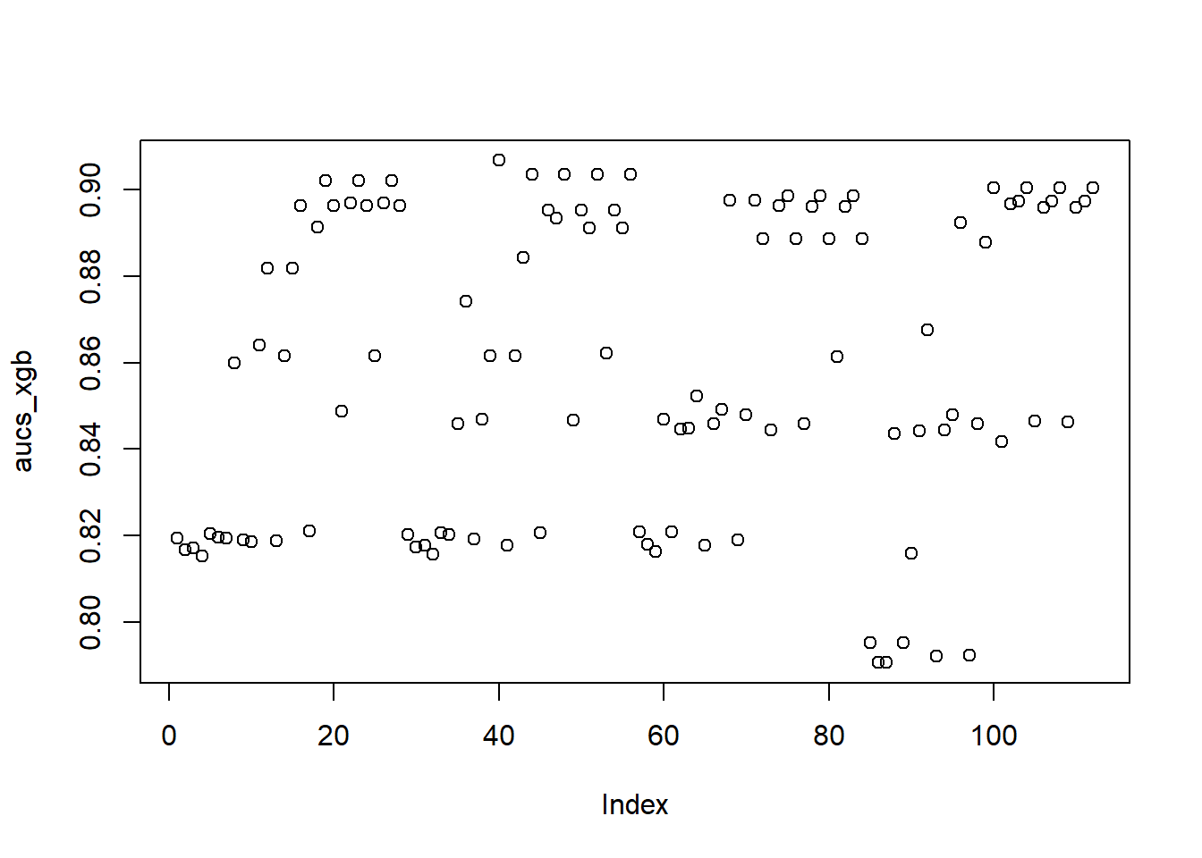
plot(aucs)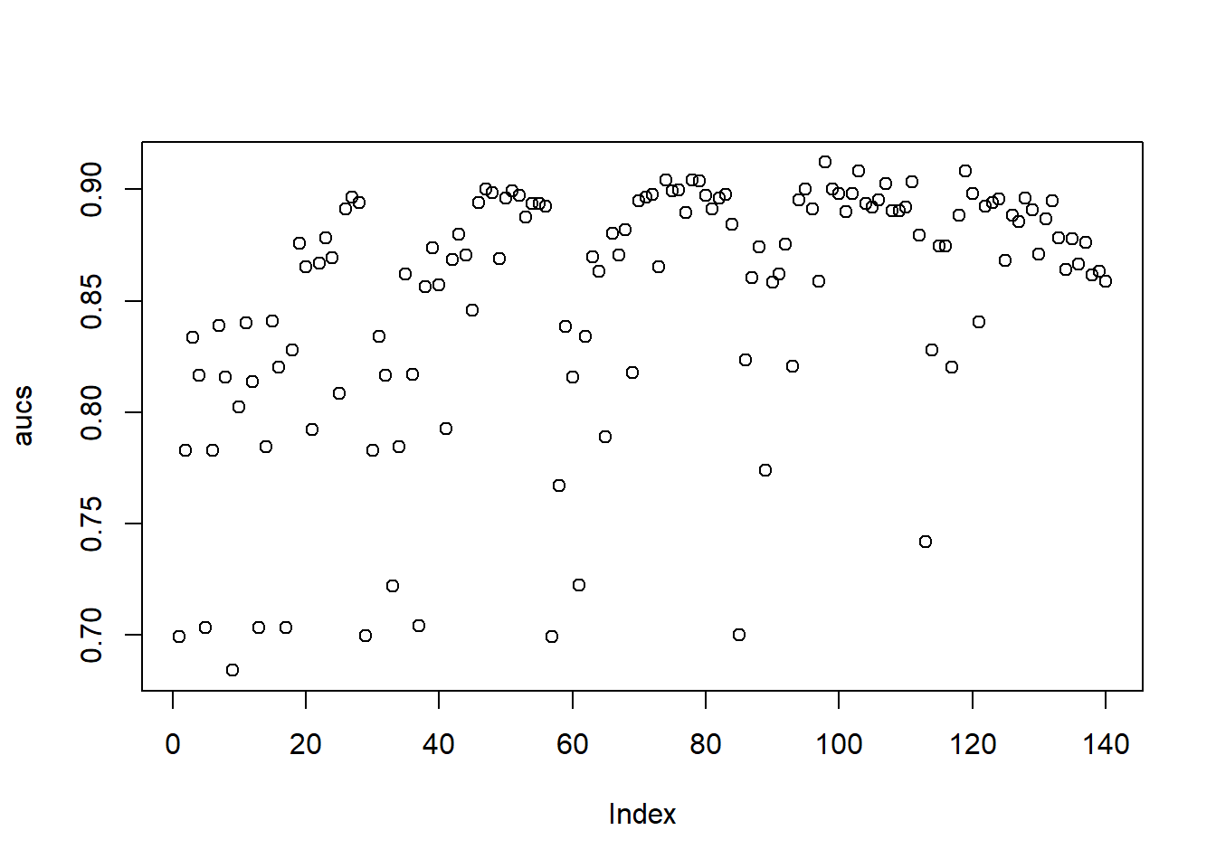
5.3.4 Catboost
One of the downside of XGBoost is that it only accepts numeric inputs and hence
all categorical features should be transformed. Most often this is done by
one-hot encoding which can lead to overfitting, especially when confronted
with high cardinality in the categories. Another downside of most gradient boosting
implementation is the fact that the gradient used in each step are estimated using the
same data points as the current model was built on, which causes a gradient bias and
leads to overfitting.
As a reaction to these downsides, catboost solves these issue by introduction
ordered target statistics for categorical variables and ordered boosting for training.
Just like xgboost, catboost is built in c++ and has wrappers for both R and Python.
Also note that catboost builds on top of the gradient boosting framework, so a
lot of hyperparameters are the same.
# CATBOOST

# First time install
# You should install the released version
# see: https://catboost.ai/en/docs/installation/r-installation-binary-installation
# First install and load devtools

#p_load(devtools)

# Now install a specific Windows version

#devtools::install_github('catboost/catboost', subdir = 'catboost/R-package')

# After installing, you can load the package
p_load(catboost)

# Transform the data to catboost format
train_pool <- catboost.load_pool(data = data.matrix(BasetableTRAINbig),
                                 label = as.numeric(as.character(yTRAINbig)))
test_pool <- catboost.load_pool(data = data.matrix(BasetableTEST),
                                 label = as.numeric(as.character(yTEST)))

# Model

# First set the parameters (set to the defaults)
# see ?catboost.train for more parameters
params = list(loss_function = 'Logloss',
              iterations = 100,
              depth = 6,
              learning_rate = 0.03,
              l2_leaf_reg = 3, #L2 regularization term for the leaf nodes (also in xgboost)
              metric_period=10)


catboost_model <- catboost.train(train_pool,  NULL,
                                 params = params)
## 0: learn: 0.6704887 total: 156ms remaining: 15.4s
## 10: learn: 0.4966705 total: 225ms remaining: 1.82s
## 20: learn: 0.3890475 total: 290ms remaining: 1.09s
## 30: learn: 0.3151809 total: 338ms remaining: 753ms
## 40: learn: 0.2657585 total: 381ms remaining: 549ms
## 50: learn: 0.2300406 total: 421ms remaining: 405ms
## 60: learn: 0.2043287 total: 463ms remaining: 296ms
## 70: learn: 0.1861820 total: 514ms remaining: 210ms
## 80: learn: 0.1720685 total: 562ms remaining: 132ms
## 90: learn: 0.1604972 total: 595ms remaining: 58.9ms
## 99: learn: 0.1529207 total: 627ms remaining: 0us# Predict
predcatboost <- catboost.predict(catboost_model, test_pool)
# Evaluate
AUC::auc(AUC::roc(predcatboost,yTEST))## [1] 0.969078Even with the default parameters catboost gives the best result. It is still possible
to tune the hyperparameters in the same way as with xgboost. The package also has
a built-in link with caret called catboost.caret which can be integrated with caret
for easy hyperparameter tuning. We refer the reader to this link.
Try further optimizing this performance as a take-home assignment.
5.4 Rotation Forest
A final ensemble model we will be covering, is the rotation forest algorithm. The algorithm extends the bagging algorithm, by for each tree we randomly cutting up the data, estimating PCA coefficients on each piece, arranging those coefficients in a matrix, and using that matrix to project data onto the principal components. Similar to random forest, you should set number of trees (parameter L) large enough (although not as high as RF).
p_load(rotationForest)
RoF <- rotationForest(x = BasetableTRAINbig, y = yTRAINbig, L = 100)
predRoF <- predict(RoF, BasetableTEST)

AUC::auc(AUC::roc(predRoF, yTEST))
## [1] 0.9727699Setting L too small would have negatively affected performance, but is much faster.
RoF <- rotationForest(x = BasetableTRAINbig, y = yTRAINbig, L = 10)
predRoF <- predict(RoF, BasetableTEST)

AUC::auc(AUC::roc(predRoF, yTEST))
## [1] 0.95554725.5 Heterogeneous ensembles
Besides some well established ensemble methods, it is always possible to combine classifiers yourself. Thereby not only using data-induced diversity, but also algorithm diversity. For instance, you can use two classifiers (random forest and xgboost) and combine them. The combination rule is to weight both predictions according to the respective AUCs. The performance in this case is slightly higher than the ones obtained individually by xgboost and random forest on themselves! (slight deviations possible due to seeding).
rFmodel <- randomForest(x = BasetableTRAINbig, y = yTRAINbig,
    ntree = 500, importance = TRUE)
predrF <- predict(rFmodel, BasetableTEST, type = "prob")[, 2]
auc_rf <- AUC::auc(AUC::roc(predrF, yTEST))

xgb <- xgb.train(data = dtrainbig, eta = optimal_params$eta,
    nrounds = optimal_params$nround, gamma = optimal_params$gamma,
    objective = "binary:logistic", verbose = 0)
predxgb <- predict(xgb, dtest)
auc_xgb <- AUC::auc(AUC::roc(predxgb, yTEST))

# Weight according to performance
finalpredictions <- (auc_rf/(auc_xgb + auc_rf)) * predrF + (auc_xgb/(auc_xgb +
    auc_rf)) * predxgb
AUC::auc(AUC::roc(finalpredictions, yTEST))
## [1] 0.9666417# Turn warnings back on
options(warn = defaultW)