6 Deep Learning
This chapter will cover the concepts seen in Session 5 Deep Learning. We will discussing two popular types of neural network architectures: classic multi-layer perceptrons and convolutional neural networks. Be aware that this is solely the tip of the iceberg and that more in detail how to implement several nonlinear models. Make sure that you go over the video and slides before going over this chapter.
6.1 Dense Neural Networks
A type of machine learning model that has gained enormous popularity during recent years are the neural networks. They can be regarded as more flexible extensions of logistic regression. A logistic regression basically is a neural network with no hidden layer and the logit function as activation function. Neural networks add hidden layers to this architecture. This is actually nothing more than a chain of logistic regressions. The length of the chain, however, enables the NN to find highly complex nonlinear relations. For specific data (e.g. longitudinal, images) there are even more specialized operations, but these fall outside of the scope of this course.
First, we will be focusing on the classical feed-forward (sequential) neural networks in this course, often referred to as a multi-layer perceptrons (MLP) or dense neural networks, referring to the sole use of dense layers in these networks (as opposed to e.g., convolutional layers). The more simple architecture also limits the settings needed for the base architecture (more elaborate measures need to be set as well, but they will be discussed later on).
To be able to work with keras make sure that you have Python (more specifically MiniConda) installed, since it will make a link between R, Python and C++. You should also have tensorflow installed, so let’s first do that to be sure that keras will work. To install tensforflow, you should also change some things to your R-session, go to: RStudio -> Tools -> Global Options -> Packages -> Disable both “Use secure download method for HTTP” and “Use Internet Explorer library/proxy for HTTP” and restart. Also make sure that you have the newest version of conda, by by running conda update -n base -c defaults conda in command line. This may take a while if this is the first time!
Let’s use the churn data from our NPC to build a neural network. As keras will automatically create a validation set, we will use BasetableTRAINbig and BasetableTEST.
# Load the tidyverse package
if (!require("pacman")) install.packages("pacman")

p_load(keras)
p_load(tensorflow)
p_load(tidyverse)

# Run this if it is the first time you use Keras in R
# install_keras()

# to install the GPU version of tensorflow/keras (although
# not needed for this course), do the following:
# install_keras(tensorflow = 'gpu') note that his will also
# only work if your PC has a GPU

# Load the datasets
load("C:\\Users\\matbogae\\OneDrive - UGent\\PPA22\\PredictiveAnalytics\\Book_2022\\data codeBook_2022\\TrainValTest.Rdata")
Recall that in the case of neural networks, you should always normalize your data to avoid computational overflow and because they are quite sensitive to to unscaled predictors. Also, the dependent variable in keras should not be set to factor but to numeric (this has to do with the fact that keras and tensorflow are actually wrapper functions are C++ code, which does not have factor-objects!). Also, keras dopes not accept a data frame so you should make a matrix
# Normalizing the data between 0 and 1
min_train <- BasetableTRAINbig %>%
    select_if(is.numeric) %>%
    sapply(., min)
max_train <- BasetableTRAINbig %>%
    select_if(is.numeric) %>%
    sapply(., max)
range_train <- max_train - min_train

# Make sure all variables are numeric
sum(sapply(BasetableTRAINbig, is.numeric)) == ncol(BasetableTRAINbig)
## [1] TRUEsum(sapply(BasetableTEST, is.numeric)) == ncol(BasetableTEST)## [1] TRUE# Normalize train
train_norm <- data.frame(BasetableTRAINbig %>%
select_if(is.numeric) %>%
scale(center = min_train, scale = range_train))
# Normalize test
test_norm <- data.frame(BasetableTEST %>%
select_if(is.numeric) %>%
scale(center = min_train, scale = range_train))
# Let's have a look whether everything is between 0 and 1
train_norm %>%
summary()## TotalDiscount TotalPrice
## Min. :0.00000 Min. :0.0000
## 1st Qu.:0.00000 1st Qu.:0.3957
## Median :0.00000 Median :0.7026
## Mean :0.02090 Mean :0.5689
## 3rd Qu.:0.01864 3rd Qu.:0.7181
## Max. :1.00000 Max. :1.0000
## TotalCredit PaymentType_DD
## Min. :0.0000 Min. :0.00000
## 1st Qu.:0.9925 1st Qu.:0.00000
## Median :1.0000 Median :0.00000
## Mean :0.9753 Mean :0.02968
## 3rd Qu.:1.0000 3rd Qu.:0.00000
## Max. :1.0000 Max. :1.00000
## PaymentStatus_Not.Paid Frequency
## Min. :0.000000 Min. :0.00000
## 1st Qu.:0.000000 1st Qu.:0.08108
## Median :0.000000 Median :0.08108
## Mean :0.005654 Mean :0.11034
## 3rd Qu.:0.000000 3rd Qu.:0.10811
## Max. :1.000000 Max. :1.00000
## Recency
## Min. :0.00000
## 1st Qu.:0.03917
## Median :0.11750
## Mean :0.16597
## 3rd Qu.:0.27846
## Max. :1.00000test_norm %>%
summary()## TotalDiscount TotalPrice
## Min. :0.00000 Min. :0.0000
## 1st Qu.:0.00000 1st Qu.:0.3960
## Median :0.00000 Median :0.7026
## Mean :0.02217 Mean :0.5621
## 3rd Qu.:0.01864 3rd Qu.:0.7181
## Max. :1.00000 Max. :0.9154
## TotalCredit PaymentType_DD
## Min. :0.0000 Min. :0.00000
## 1st Qu.:0.9949 1st Qu.:0.00000
## Median :1.0000 Median :0.00000
## Mean :0.9728 Mean :0.03253
## 3rd Qu.:1.0000 3rd Qu.:0.00000
## Max. :1.0000 Max. :1.00000
## PaymentStatus_Not.Paid Frequency
## Min. :0.000000 Min. :0.00000
## 1st Qu.:0.000000 1st Qu.:0.08108
## Median :0.000000 Median :0.08108
## Mean :0.001414 Mean :0.11055
## 3rd Qu.:0.000000 3rd Qu.:0.10811
## Max. :1.000000 Max. :1.00000
## Recency
## Min. :0.00000
## 1st Qu.:0.03917
## Median :0.10649
## Mean :0.15365
## 3rd Qu.:0.25581
## Max. :0.49327# Make a matrix
x_trainNN <- train_norm %>%
as.matrix()
x_testNN <- test_norm %>%
as.matrix()
# Set the ytrain and ytest to numeric
y_trainNN <- yTRAINbig %>%
as.character() %>%
as.numeric()
y_testNN <- yTEST %>%
as.character() %>%
as.numeric()Now that our data is in the right format, we can move on to building our network’s architecture. We already discussed how neural networks are structured: you start with one input layer (your independent variables), followed by one or multiple hidden layers (each with a specific number of nodes) and end with the output layer (dependent; our digits). The input and the output layer are fixed, based on what you feed to the network. This means that what you ‘build’ is the network’s hidden layer structure. More hidden layers mean a more complex relationship, as do more nodes per layer. This match between model complexity and en true relationship between x and y is even more complicated for neural networks, as much more variance in model specification is possible. This is why neural network developers often monitor over- and underfitting even more closely. The general rule is that you should first find a model structure that is complex enough to overfit (i.e., complex enough to find true relation) and then tweak this towards a structure that stops from overfitting.
Let us start with a simple network architecture. First start by declaring that you are building a simple sequential network. Then add a first hidden dense layer with 32 nodes. Note how the input is equal to number of values in the input vector (7). A second hidden layer is added with 16 nodes. Finally, we add the output layer with 1 unit and use the sigmoid activiation function.
We want to make several remarks about this architecture’s details. Note how the hidden layers use the rectified linear unit (see theory) as activation function to avoid vanishing gradients. The output layer uses the sigmoid function. This is because the sigmoid function squeezes the output between 0 and 1 and that is exactly what we want (just as in logistic regression!). Since we are using a limited number of variables, the architecture does not strictly narrow down in size (7-32-16-1). However, architecture become more shallow by the end of the network. This because you use the hidden layer to learn latent features (e.g., bends and right corners in our example), while near the end you use those latent features to predict the outcome.
# don't mind the errors
model <- keras_model_sequential()
## Loaded Tensorflow version 2.7.0model %>%
layer_dense(units = 32, activation = "relu", input_shape = c(7)) %>%
layer_dense(units = 16, activation = "relu") %>%
layer_dense(units = 1, activation = "sigmoid")
# Have a look at your model
summary(model)## Model: "sequential"
## __________________________________________________
## Layer (type) Output Shape Param #
## ==================================================
## dense_2 (Dense) (None, 32) 256
##
## dense_1 (Dense) (None, 16) 528
##
## dense (Dense) (None, 1) 17
##
## ==================================================
## Total params: 801
## Trainable params: 801
## Non-trainable params: 0
## __________________________________________________It may seem that we are now ready to fit the model. However, we first need to compile the model. This is where you need to configure the learning process, which is done via the compile() function. It receives three arguments:
An optimizer. This could be the string identifier of an existing optimizer (e.g. as “rmsprop”, “adam”, or “adagrad”) or a call to an optimizer function (e.g.
optimizer_sgd()).A loss function. This is the objective that the model will try to minimize. It can be the string identifier of an existing loss function (e.g. “categorical_crossentropy” or “mse”) or a call to a loss function (e.g.
loss_mean_squared_error()).A list of metrics. For many classification problem you will want to set this to
metrics = c('accuracy'). A metric could be the string identifier of an existing metric or a call to metric function (e.g.metric_binary_crossentropy()). This metric is not what is optimized during the learning phase (this is the loss function) but the metric which is reported. To have a more elaborate choice of metrics, you can go call thetfobject (e.g., to implement the AUC usekeras$metrics$AUC()). As we are more interested in optimizing in terms of AUC, we will use this as our metric.
model %>%
    compile(loss = "binary_crossentropy", optimizer = optimizer_adam(),
        metrics = keras$metrics$AUC())
We will now actually fit the model. This is done with 30 epochs, on a batch size of 128. An epoch is how many times the algorithm iterates over the total data. Remember: we use an iterative optimizer, so each data point is fed to the optimizer 30 times. This is done with 128 data points simultaneously (batch size). We use 20% of x_trainNN object for model validation.
# fit
history <- model %>%
    fit(x_trainNN, y_trainNN, epochs = 30, batch_size = 128,
        validation_split = 0.2, verbose = 0)

# Plot an overview of the performance
plot(history)
## `geom_smooth()` using formula 'y ~ x'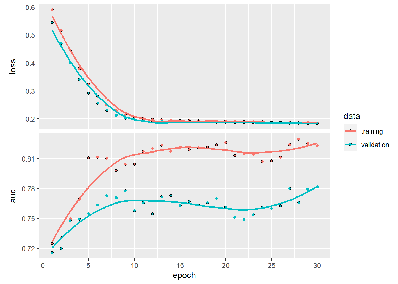
Do you observe how the training loss keeps on decreasing and the validation loss actually also drecreases. However, when looking at the AUC, we see a different story, while training increases, the validation set stagnates (depending on the run it can be more clear cut).This could actually mean two things: you should increase the number of epoch or you are overfitting.
We will assume that this is overfitting and use dropout layers. Dropout works by randomly setting the outgoing edges of hidden units (neurons that make up hidden layers) to 0 at each update of the training phase. Doing so, it prevents the algorithm from learning unnecessary links. We will use dropout rates (rate of nodes set at 0) of 10% and 10% on the first and second hidden layers, respectively.
model <- keras_model_sequential()
model %>%
    layer_dense(units = 32, activation = "relu", input_shape = c(7)) %>%
    layer_dropout(rate = 0.4) %>%
    layer_dense(units = 16, activation = "relu") %>%
    layer_dropout(rate = 0.3) %>%
    layer_dense(units = 1, activation = "sigmoid")

model %>%
    compile(loss = "binary_crossentropy", optimizer = optimizer_adam(),
        metrics = keras$metrics$AUC())
history <- model %>%
fit(x_trainNN, y_trainNN, epochs = 30, batch_size = 128,
validation_split = 0.2, verbose = 0)plot(history)## `geom_smooth()` using formula 'y ~ x'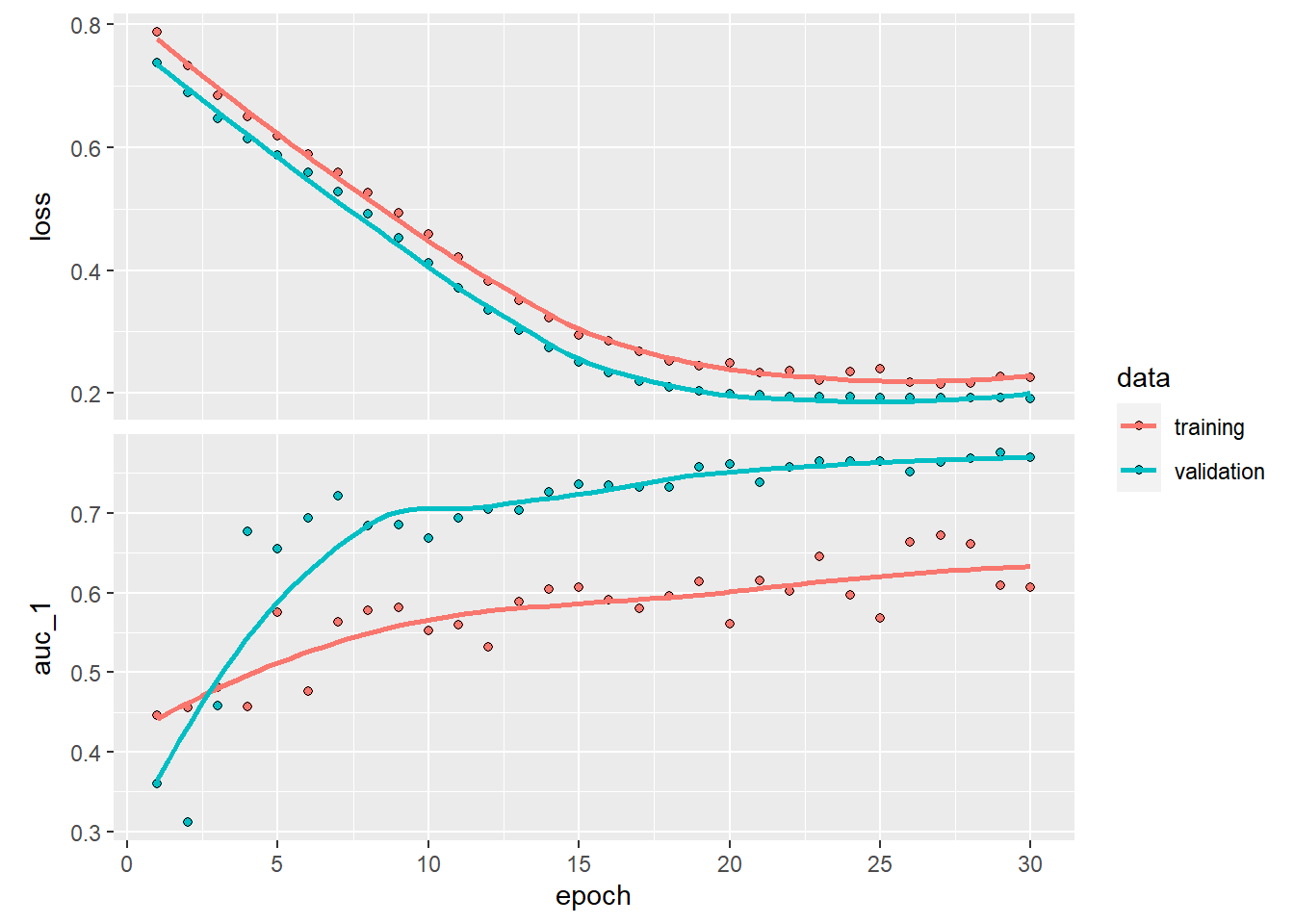
While the training set is now bumpier, we see that the validation set becomes more stable thanks to dropout! Play around a bit with the parameters to see if you can find better drop out rates or just even play around with number of layers or epochs.
To have the performance on the test set, we can easily use some built-in keras to have the performance as defined by the specified metrics and loss functions.
model %>%
    keras::evaluate(x_testNN, y_testNN)
## loss auc_1
## 0.1873585 0.8877062If you would check the final AUC of this model and the model without dropout you will see that the performance improved thanks to dropout.
If you want to plot a classic roc plot, you should do the following:
p_load(AUC)

predictionsNN <- model %>%
    predict(x_testNN)
plot(roc(predictionsNN, yTEST))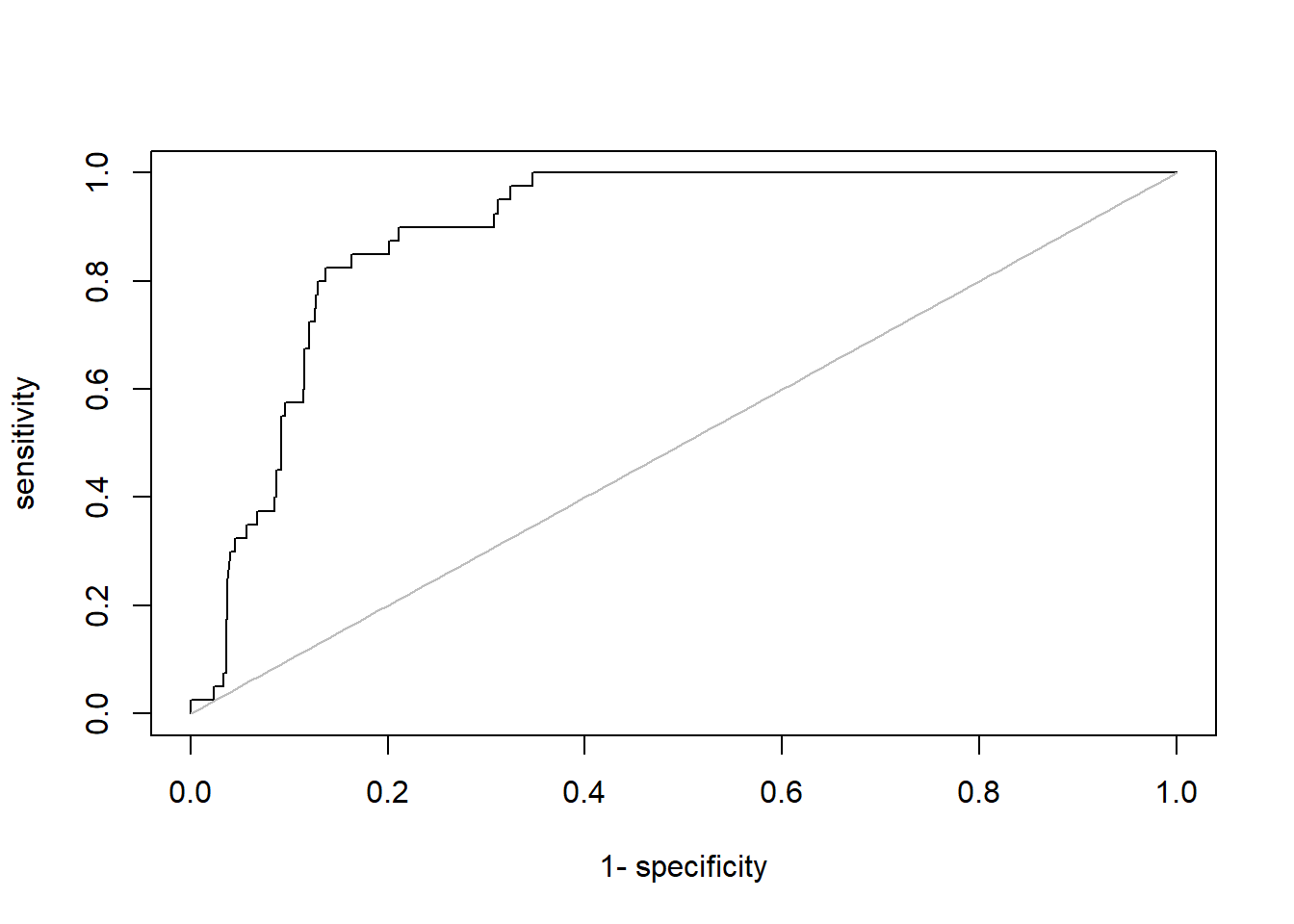
There are several other packages in R available to make neural nets, however none of them have the flexibility of keras. One famous package is the nnet package, which builds a neural network with one hidden layer and the sigmoid activation function with regularization. As you can already notice, the options are limited compared to keras. For the sake of completeness, we will show how the nnet package works.
p_load(nnet)

# first we need to scale the data to range [0,1] avoid
# numerical problems
BasetableTRAINnumID <- sapply(BasetableTRAIN, is.numeric)
BasetableTRAINnum <- BasetableTRAIN[, BasetableTRAINnumID]
minima <- sapply(BasetableTRAINnum, min)
scaling <- sapply(BasetableTRAINnum, max) - minima

# ?scale center is subtracted from each column.  Because we
# use the minima this sets the minimum to zero. scale: each
# column is divided by scale.  Because we use the range
# this sets the maximum to one.
BasetableTRAINscaled <- data.frame(base::scale(BasetableTRAINnum,
    center = minima, scale = scaling), BasetableTRAIN[, !BasetableTRAINnumID])
colnames(BasetableTRAINscaled) <- c(colnames(BasetableTRAIN)[BasetableTRAINnumID],
    colnames(BasetableTRAIN)[!BasetableTRAINnumID])

# Set paramaters of nnet
NN.rang <- 0.5  #the range of the initial random weights parameter
NN.maxit <- 10000  #set high in order not to run into early stopping
NN.size <- c(5, 10, 20)  #number of units in the hidden layer
NN.decay <- c(0, 0.001, 0.01, 0.1)  #weight decay.

# Same as lambda in regularized LR. Controls overfitting
call <- call("nnet", formula = yTRAIN ~ ., data = BasetableTRAINscaled,
    rang = NN.rang, maxit = NN.maxit, trace = FALSE, MaxNWts = Inf)
tuning <- list(size = NN.size, decay = NN.decay)

# tune nnet scale validation data
BasetableVALIDATEnum <- BasetableVAL[, BasetableTRAINnumID]
BasetableVALIDATEscaled <- data.frame(base::scale(BasetableVALIDATEnum,
    center = minima, scale = scaling), BasetableVAL[, !BasetableTRAINnumID])
colnames(BasetableVALIDATEscaled) <- colnames(BasetableTRAINscaled)

# Make a convenience function to help you with the tuning
# Same function as used for SVM in Advanced Modeling
# section
tuneMember <- function(call, tuning, xtest, ytest, predicttype = NULL,
    probability = TRUE) {
    if (require(AUC) == FALSE)
        install.packages("AUC")
    library(AUC)

    grid <- expand.grid(tuning)

    perf <- numeric()
    for (i in 1:nrow(grid)) {
        Call <- c(as.list(call), grid[i, ])
        model <- eval(as.call(Call))

        predictions <- predict(model, xtest, type = predicttype,
            probability = probability)

        if (class(model)[2] == "svm")
            predictions <- attr(predictions, "probabilities")[,
                "1"]

        if (is.matrix(predictions))
            if (ncol(predictions) == 2)
                predictions <- predictions[, 2]
        perf[i] <- AUC::auc(roc(predictions, ytest))
    }
    perf <- data.frame(grid, auc = perf)
    perf[which.max(perf$auc), ]
}

(result <- tuneMember(call = call, tuning = tuning, xtest = BasetableVALIDATEscaled,
    ytest = yVAL, predicttype = "raw"))
## size decay auc
## 9 20 0.01 0.9133936# Create final model
BasetableTRAINbignum <- BasetableTRAINbig[, BasetableTRAINnumID]
BasetableTRAINbigscaled <- data.frame(base::scale(BasetableTRAINbignum,
center = minima, scale = scaling), BasetableTRAINbig[, !BasetableTRAINnumID])
colnames(BasetableTRAINbigscaled) <- c(colnames(BasetableTRAINbig)[BasetableTRAINnumID],
colnames(BasetableTRAINbig)[!BasetableTRAINnumID])
NN <- nnet(yTRAINbig ~ ., BasetableTRAINbigscaled, size = result$size,
rang = NN.rang, decay = result$decay, maxit = NN.maxit, trace = TRUE,
MaxNWts = Inf)## # weights: 181
## initial value 1656.772273
## iter 10 value 300.571846
## iter 20 value 224.983357
## iter 30 value 213.925727
## iter 40 value 206.915331
## iter 50 value 196.407848
## iter 60 value 188.327624
## iter 70 value 183.160890
## iter 80 value 180.268069
## iter 90 value 177.557398
## iter 100 value 174.782883
## iter 110 value 170.589488
## iter 120 value 168.641031
## iter 130 value 166.923742
## iter 140 value 165.398050
## iter 150 value 164.427990
## iter 160 value 163.863965
## iter 170 value 163.394400
## iter 180 value 163.131216
## iter 190 value 162.905513
## iter 200 value 162.460363
## iter 210 value 161.951709
## iter 220 value 161.550895
## iter 230 value 161.335257
## iter 240 value 161.247130
## iter 250 value 161.206185
## iter 260 value 161.190859
## iter 270 value 161.180768
## iter 280 value 161.173839
## iter 290 value 161.168778
## iter 300 value 161.165511
## iter 310 value 161.163165
## iter 320 value 161.160422
## iter 330 value 161.157610
## iter 340 value 161.154707
## iter 350 value 161.151845
## iter 360 value 161.149181
## iter 370 value 161.147031
## iter 380 value 161.140910
## iter 390 value 161.124036
## iter 400 value 161.119115
## iter 410 value 161.114372
## iter 420 value 161.111686
## iter 430 value 161.109722
## iter 440 value 161.108910
## iter 450 value 161.108677
## iter 460 value 161.108614
## iter 470 value 161.108530
## iter 480 value 161.108423
## iter 490 value 161.108366
## final value 161.108353
## converged# predict on test
BasetableTESTnum <- BasetableTEST[, BasetableTRAINnumID]
BasetableTESTscaled <- data.frame(base::scale(BasetableTESTnum,
center = minima, scale = scaling), BasetableTEST[, !BasetableTRAINnumID])
colnames(BasetableTESTscaled) <- c(colnames(BasetableTRAINbig)[BasetableTRAINnumID],
colnames(BasetableTRAINbig)[!BasetableTRAINnumID])
predNN <- as.numeric(predict(NN, BasetableTESTscaled, type = "raw"))
AUC::auc(roc(predNN, yTEST))## [1] 0.9593328As you can see performance is better than the keras example. This can be because your specifications in the keras model were too complex for this problem. Remember that a one hidden layer neural network with several hidden nodes serve as universal approximators, especially in business functions. So in contrast to the popular opinion that more complex NNs are always better, this does not hold on tabular business data. You can of course try to recreate this network in keras and see what you get.
6.2 Convolutional Neural Networks
In this part, we will focus on convolutional neural network (CNN) architectures, which can learn local, spatial structures within data. This also entails that those structures should be present in your data. Our NPC churn example might not be the ideal data set for this, as those features are relatively independent from each other. In fact, in traditional machine learning, we generally want features to be independent from each other, as this improves the interpretability of our model. However, CNNs will leverage dependencies between single features. A typical example is image data, where each feature represents a pixel. These pixels are not very informative on their own. Rather, the combination (structures) of pixels form informative aspects (e.g., certain curves). This automated creation of informative aspects from non-informative features is called feature extraction or automated feature engineering and is one of the reasons why deep learning is so hyped up currently. As remember: the largest part of your work is typically pre-processing. Sometimes, good NN architectures can do this for you. Can you imagine how hard it would be to code meaningful features from image pixels? This actually how it was done up until two decades ago. However, CNN applications are not limited to image classification tasks. While it is the most popular one, and also one which is immensely important for several exciting new innovations (self-driving cars, Amazon Go, etc.), they can be used for any problem in which the location of a feature is relevant. Examples include time series (data is well-ordered; 1D convolution preferred) and weather forecasts.
Consider the weather forecasts: You would need to build a map of the current weather conditions (location-based values, but not actual images). If you add another dimension to it for the previous weather maps (chronologically) and you have a 4–d convolution problem to predict the weather.
However, strict business applications are also feasible. Consider a situation where you are a real estate investment company. The value of real estate is highly influenced by its location. Location is a 2D structured data format. These structures, and evolutions through time (e.g., gentrification), may be used to predict the future average house prices at different locations.
Despite the numerous applications, we will be focusing on the most popular application: image classification. Doing so, we will show how much better CNNs are at this job than regular DNNs. Do note that the we are handling a multi-class problem now rather than a binary one. Luckily, this is easily adapted in Keras by using 10 output nodes. We will be using the MNIST dataset, which is one of the most famous datasets in the world (you could say the hello world of deep learning). It includes a large number of pictures of hand-written numbers, with their numeric value as dependent feature. First let us start by reading in the data. Luckily, the dataset is so popular, that is already automatically included in keras. To read it in, we will be using the dataset_mnist() function. On top of this, the data is also already split up Note how a random forest or DNN cannot understand structure. We need to feed it to them in an ustructured way. This is done through the array_reshape() function. We also scale the (grey-scale) images by dividing their pixel values. Note how an RGB image would have 3 times as much dimensions. Also note how we plot a random hand-written digit (i.e., the eighth observation in the training sample) before this restructuring. This to give you some insights about the dataset used. Feel free to plot some more digits if you’d like.
# Load the data
mnist <- dataset_mnist()

c(c(train_images, train_labels), c(test_images, test_labels)) %<-%
    mnist

# Plot the eight digit
digit <- train_images[8, , ]
plot(as.raster(digit, max = 255))
# Reshape the data to proper format
train_images <- array_reshape(train_images, c(60000, 28 * 28))
train_images <- train_images/255

test_images <- array_reshape(test_images, c(10000, 28 * 28))
test_images <- test_images/255

train_labels <- to_categorical(train_labels)
test_labels <- to_categorical(test_labels)
Before we will dive into the actual modeling of a CNN, let us first construct and evaluate our baseline model. We build a DNN, compile it, and let it fit on the training data.
# Build architecture
dnn <- keras_model_sequential() %>%
    layer_dense(units = 512, activation = "relu", input_shape = c(784)) %>%
    layer_dense(units = 10, activation = "softmax")

# Compile with same settings as before
dnn %>%
    compile(loss = "binary_crossentropy", optimizer = optimizer_adam(),
        metrics = keras$metrics$AUC())

# Fit to training data
history_dnn <- dnn %>%
    fit(train_images, train_labels, epochs = 30, batch_size = 128,
        validation_split = 0.2, verbose = 0)

plot(history_dnn)
## `geom_smooth()` using formula 'y ~ x'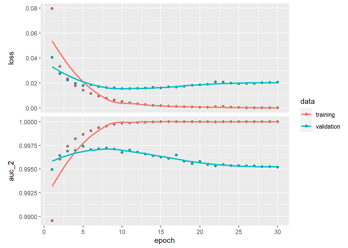
dnn %>%
    keras::evaluate(test_images, test_labels)
## loss auc_2
## 0.01670339 0.99646938This is already rather an impressive performance right? However, in the validation plot we see that the model starts to overfit at epoch > 10. To give the DNN a chance as fair as possible, we are going to stop after 10 epochs.
# Build architecture
dnn <- keras_model_sequential() %>%
    layer_dense(units = 512, activation = "relu", input_shape = c(784)) %>%
    layer_dense(units = 10, activation = "softmax")

# Compile with same settings as before
dnn %>%
    compile(loss = "binary_crossentropy", optimizer = optimizer_adam(),
        metrics = c("accuracy", keras$metrics$AUC()))

# Fit to training data
history_dnn <- dnn %>%
    fit(train_images, train_labels, epochs = 10, batch_size = 128,
        validation_split = 0.2, verbose = 0)

plot(history_dnn)
## `geom_smooth()` using formula 'y ~ x'
dnn %>%
    keras::evaluate(test_images, test_labels)
## loss accuracy auc_3
## 0.01423233 0.98229998 0.99740845Most of you will probably think that this performance is already unbeatable. However, think back about how computer vision is used. Would it be satisfying if a self-driving car only hits 2% of pedestrians crossing the road? It may depend on what you value in life, but let’s say it would not be desirable to most of us. On top of this, it is not hard to imagine that the complex task of identifying all objects on the road is harder than simply determining what number we are seeing.
We now know how our structure-unaware model performs. Let’s now try this out with a structure-aware CNN. Of course, this also entails that we should use the data in its structured form. This means that, rather than a (sample_size, number_pixels)=(60000, 28*28) dimensionality, we will be using a (sample_size, height, width, colour_channels)=(60000, 28, 28, 1) dimensionality.
# Reload data
mnist <- dataset_mnist()

c(c(train_images, train_labels), c(test_images, test_labels)) %<-%
    mnist

# Put data in the correct shape
train_images <- array_reshape(train_images, c(60000, 28, 28,
    1))
train_images <- train_images/255

test_images <- array_reshape(test_images, c(10000, 28, 28, 1))
test_images <- test_images/255

train_labels <- to_categorical(train_labels)
test_labels <- to_categorical(test_labels)
Let us start by the essence of a CNN: the convolutional layers.
cnn <- keras_model_sequential() %>%
    layer_conv_2d(filters = 32, kernel_size = c(3, 3), activation = "relu",
        input_shape = c(28, 28, 1)) %>%
    layer_max_pooling_2d(pool_size = c(2, 2)) %>%
    layer_conv_2d(filters = 64, kernel_size = c(3, 3), activation = "relu") %>%
    layer_max_pooling_2d(pool_size = c(2, 2)) %>%
    layer_conv_2d(filters = 64, kernel_size = c(3, 3), activation = "relu")

# Display current architecture
cnn
## Model
## Model: "sequential_4"
## __________________________________________________
## Layer (type) Output Shape Param #
## ==================================================
## conv2d_2 (Conv2D) (None, 26, 26, 32) 320
##
## max_pooling2d_1 (Max (None, 13, 13, 32) 0
## Pooling2D)
##
## conv2d_1 (Conv2D) (None, 11, 11, 64) 18496
##
## max_pooling2d (MaxPo (None, 5, 5, 64) 0
## oling2D)
##
## conv2d (Conv2D) (None, 3, 3, 64) 36928
##
## ==================================================
## Total params: 55,744
## Trainable params: 55,744
## Non-trainable params: 0
## __________________________________________________This already looks nice, but what are we exactly doing? We are creating 3 convolutional layers. The first one by using 32 filters/kernels, the second and third one by using 64 filters each. We can use the term filters/kernels interchangeably here as we are working with 2D convolutional layers (layer_conv_2d), as the images have no third dimension due to being greyscale rather than coloured. Note how the width and height decrease drastically from the initial 28x28 image input to a 3x3 output in the last convolutional layer. This is because of two effects: the absence of padding and max-pooling.
First let’s start with padding, which happens within the convolutional layer. The fact that we did not use padding entails that we ‘lose’ 2 units due to border effects: the ‘borders’ of our 28x28 grid. The max pooling, as seen in theory, ‘pools’ all the individual features per pool into one feature. Because we use pool_size = c(2, 2), we only retain one value per 2x2 grid. This results into a 13x13 grid downsizing from the initial 26x26 grid. Eventually, we will have 64 3x3 filters which should encode all edges and curves that form hand-written digits.
Does this mean that we can start fitting this archictecture? NO! Our output currently consists of ‘forms’ rather than a 10-class classification. To solve this, we stack some dense layers on top of the convolutional layers. In fact, we now are building a dense net, which uses the ‘automatically learned’ features from the convolutional layers as input. Note how this entails that we also have to restructure our input again with the layer_flatten() function.
cnn <- cnn %>%
    layer_flatten() %>%
    layer_dense(units = 64, activation = "relu") %>%
    layer_dense(units = 10, activation = "softmax")

# Compile with same settings as before
cnn %>%
    compile(loss = "binary_crossentropy", optimizer = optimizer_adam(),
        metrics = c("accuracy", keras$metrics$AUC()))

# Fit to training data
history_cnn <- cnn %>%
    fit(train_images, train_labels, epochs = 10, batch_size = 128,
        validation_split = 0.2, verbose = 0)

plot(history_cnn)
## `geom_smooth()` using formula 'y ~ x'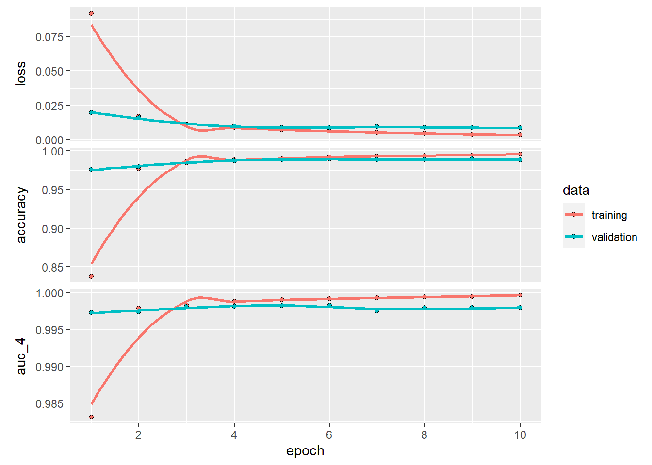
cnn %>%
    keras::evaluate(test_images, test_labels)
## loss accuracy auc_4
## 0.006107754 0.990800023 0.998665750I guess you now all know why deep learning developers work with GPU…
We improved both AUC and accuracy, and while these improvements may seem small, we reduced our error rate (accuracy) by 27%! On top of this, we did not give the CNN a fair enough chance, as we did not use our validation curves similarly as we did for the DNN. The curves suggest an ideal number of epochs around 5.
# Fit to training data
history_cnn <- cnn %>%
    fit(train_images, train_labels, epochs = 5, batch_size = 128,
        validation_split = 0.2, verbose = 0)

plot(history_cnn)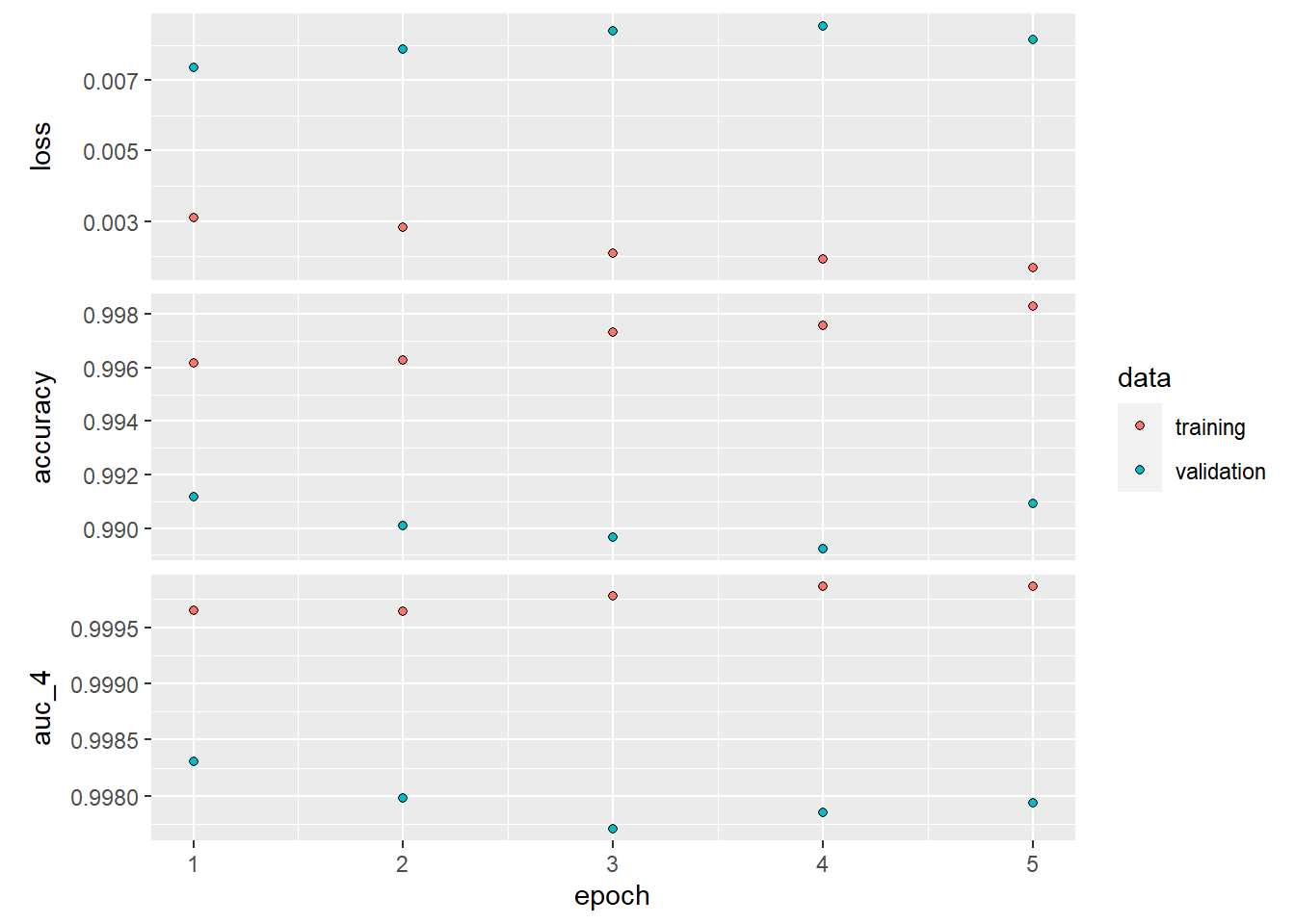
cnn %>%
    keras::evaluate(test_images, test_labels)
## loss accuracy auc_4
## 0.006429495 0.992200017 0.998439848A simple repeat of the dense network methodology (with semi-optimized epochs) ensured a reduction in error rate of 49% ((0.991299987-0.98269999)/(1-0.98269999))! Now we sure have reached the full potential of a simple convnet right? Well we might be still be able to improve our model with a simple altering in our approach. We limited our epochs to 5 as we noticed overfitting afterwards. Overfitting is caused by having too few samples to learn from, rendering you unable to train a model that can generalize to new data. Given infinite data, your model would be exposed to every possible aspect of the data distribution at hand: you would never overfit. Data augmentation takes the approach of generating more training data from existing training samples, by augmenting the samples via a number of random transformations that yield believable-looking images. The goal is that at training time, your model will never see the exact same picture twice. This helps expose the model to more aspects of the data and generalize better.
In Keras, this can be done by configuring a number of random transformations to be performed on the images read by an image_data_generator. Let’s get started with an example.
datagen <- image_data_generator(rescale = 1/255, rotation_range = 40,
    width_shift_range = 0.2, height_shift_range = 0.2, shear_range = 0.2,
    zoom_range = 0.2, horizontal_flip = TRUE, fill_mode = "nearest")
These are just a few of the options available (for more, see the Keras documentation).
Let’s quickly go over this code:
rotation_range is a value in degrees (0–180), a range within which to randomly rotate pictures.
width_shift_range and height_shift_range are ranges (as a fraction of total width or height) within which to randomly translate pictures vertically or horizontally.
shear_range is for randomly applying shearing transformations.
zoom_range is for randomly zooming inside pictures.
horizontal_flip is for randomly flipping half the images horizontally—relevant when there are no assumptions of horizontal asymmetry (for example, real-world pictures).
fill_mode is the strategy used for filling in newly created pixels, which can appear after a rotation or a width/height shift.
We will now augment the data. Note how we have to input the datagen image generator into the flow_images_from_data() function which continuously randomly deploys this on the training data in the fitting through the fit_generator() step.
cnn## Model
## Model: "sequential_4"
## __________________________________________________
## Layer (type) Output Shape Param #
## ==================================================
## conv2d_2 (Conv2D) (None, 26, 26, 32) 320
##
## max_pooling2d_1 (Max (None, 13, 13, 32) 0
## Pooling2D)
##
## conv2d_1 (Conv2D) (None, 11, 11, 64) 18496
##
## max_pooling2d (MaxPo (None, 5, 5, 64) 0
## oling2D)
##
## conv2d (Conv2D) (None, 3, 3, 64) 36928
##
## flatten (Flatten) (None, 576) 0
##
## dense_11 (Dense) (None, 64) 36928
##
## dense_10 (Dense) (None, 10) 650
##
## ==================================================
## Total params: 93,322
## Trainable params: 93,322
## Non-trainable params: 0
## __________________________________________________datagen <- image_data_generator(rotation_range = 40, width_shift_range = 0.2,
height_shift_range = 0.2, shear_range = 0.2, zoom_range = 0.2,
horizontal_flip = TRUE)
train_generator <- flow_images_from_data(x = train_images, y = train_labels,
datagen, batch_size = 128)
history_cnn <- cnn %>%
fit(train_generator, steps_per_epoch = 300, epochs = 20,
verbose = 0)
cnn %>%
keras::evaluate(test_images, test_labels)## loss accuracy auc_4
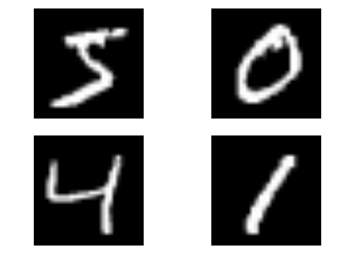
## 0.01386008 0.97869998 0.99729449This is not what we wanted! The performance is lower! What causes this? Let us check some original images and some augmented images.
op <- par(mfrow = c(2, 2), pty = "s", mar = c(1, 0, 1, 0))
for (i in 1:4) {
    plot(as.raster(train_images[i, , , ]))
}
par(op)datagen <- image_data_generator(rotation_range = 40, width_shift_range = 0.2,
height_shift_range = 0.2, shear_range = 0.2, zoom_range = 0.2,
horizontal_flip = TRUE)
train_generator <- flow_images_from_data(x = train_images, y = train_labels,
datagen, batch_size = 128)
op <- par(mfrow = c(2, 2), pty = "s", mar = c(1, 0, 1, 0))
batch <- generator_next(train_generator)
for (i in 1:4) {
plot(as.raster(batch[[1]][i, , , ]))
}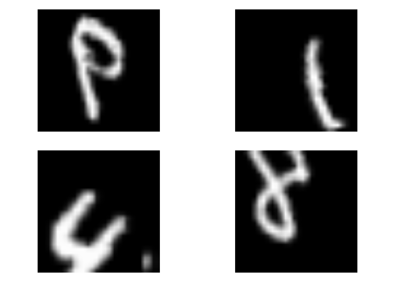
par(op)The images are becoming too different! Especially the horizontal_flip is giving some undesired effects: how should the algorithm now know the difference between a 6 or a 9? Let us tone down the data augmentation a bit and see the effect on performance.
datagen <- image_data_generator(rotation_range = 10, width_shift_range = 0.1,
    height_shift_range = 0.1, shear_range = 0.1, zoom_range = 0.1,
    horizontal_flip = FALSE)

train_generator <- flow_images_from_data(x = train_images, y = train_labels,
    datagen, batch_size = 128)

history_cnn <- cnn %>%
    fit(train_generator, steps_per_epoch = 300, epochs = 20,
        verbose = 0)

cnn %>%
    keras::evaluate(test_images, test_labels)
## loss accuracy auc_4
## 0.005147649 0.992200017 0.998985648All right, this is really nice. With an accuracy of 99.5%, we have incredibly improved from the initial performance of around 98%.