3 Modeling and Evaluation
This chapter will cover the main concepts seen in Modeling and Evaluation. We will discuss the basic experimental set-up, the bias-variance trade-off, the most important performance metrics and finally go over the workhorse models in predictive analytics (linear/logistic regression and decision trees). Make sure that you go over the video and slides before going over this chapter.
3.1 Experimental set-up
The first part is about experimental set-up. Remember that we always want to have an idea about how well our model will perform in our specific situation. Ideally, you should know this before we deploy the model, as otherwise we might get an upleasant surprise at the end of the road. Evaluating model performance always needs to be done on unseen data, as evaluating your model on seen data is some sort of self-fulfilling prophecy. You will most likely be correct because you learn patterns on the same data you are checking the validity of those patterns! For example, when you have some elder people in your data set and all are observed to churnk, your model will then always predict elder people to be churners. The question now arises: is this really the true relationship? The answer is of course: no! Unseen data helps in evaluating whether learned patterns occur outside training samples. But how do you get unseen data? The most typical method is to divide your data into chunks you use to learn and chunks you use to evaluate. While this principle is rather straight-forward, several methods exist to split into learning and evaluation chunks. We will guide you through the most important ones.
For the sake of this exercise, we will be using a churn dataset with solely the traditional RFM and LOR variables. Hence, the data is different from Preprocessing section, as we wanted a more compact data set for our modeling exercises and also have some more data points. However, a good exercise could be to use the final data set in the Preprocessing section and see what changes.
Let’s start with reading in our data from disk and change the data type of the dependent variable (churn) from integer to factor. The reason behind this is simply the fact that the used package requires you to do so for classification tasks.
# Load the tidyverse package
if (!require("pacman")) install.packages("pacman")
require("pacman", character.only = TRUE, quietly = TRUE)
p_load(tidyverse)

# Set seed to make results reproducible
set.seed(123)

# Read in the data from disk
basetable <- read_csv(file = "C:\\Users\\matbogae\\OneDrive - UGent\\PPA22\\PredictiveAnalytics\\Book_2022\\data codeBook_2022\\basetable.csv")
## Rows: 41739 Columns: 5## -- Column specification --------------------------
## Delimiter: ","
## dbl (5): Monetary_score, Total_quantity, recen...##
## i Use `spec()` to retrieve the full column specification for this data.
## i Specify the column types or set `show_col_types = FALSE` to quiet this message.# Set churn as factor
basetable$churn <- as.factor(basetable$churn)
# Have glimpse at the data
basetable %>%
glimpse()## Rows: 41,739
## Columns: 5
## $ Monetary_score <dbl> 12519.00, 7315.20, 3267.8~
## $ Total_quantity <dbl> 715, 309, 176, 74, 390, 1~
## $ recency_score <dbl> 16, 36, 15, 21, 1, 22, 50~
## $ days_customer <dbl> 15503, 16964, 22442, 1659~
## $ churn <fct> 0, 0, 0, 0, 0, 0, 0, 0, 0~The holdout set
We start with the most simple implementation: dividing into 1 training chunk (training set) and one evaluation chunk (test set). To do so, we create a vector (allind) which samples all the indicators (row numbers) of the overall basetable. By sampling without replacement, we get all the indices in a random order. If we take the first half of allind, we get two random halfs of indices (trainind & testind), by subsetting the data according to these indices we get a randomized 50/50 train/test split! Note how we can easily adapt the 50/50 ratio to a different ratio as indicated by the commented code.
# create idicators randomize order of indicators
allind <- sample(x = 1:nrow(basetable), size = nrow(basetable))

# split in two equal parts
trainind <- allind[1:round(length(allind) * 0.5)]
testind <- allind[(round(length(allind) * (0.5)) + 1):length(allind)]

# alternative split 60/40 split trainind <-
# allind[1:round(length(allind)*0.6)] testind <-
# allind[round(length(allind)*(0.6))+1:length(allind)]

# actual subsetting
train <- basetable[trainind, ]
test <- basetable[testind, ]

nrow(train)
## [1] 20870nrow(test)## [1] 20869What should we do if we want to compare different parameter settings, algorithms, etc? If we would compare them to test set, we would select the one that has the best fit to the test set, while in fact we want the one that has the best performance on the truly unknown and unseen new data in our purpose model. Evaluating all on the test set is likely to result in an over-evaluation of the model’s performance. This is why we need a third validation set to validate different settings on, before we evaluate (test) on the test set.
# create idicators randomize order of indicators
allind <- sample(x = 1:nrow(basetable), size = nrow(basetable))

# split in three parts
trainind <- allind[1:round(length(allind)/3)]
valind <- allind[(round(length(allind)/3) + 1):round(length(allind) *
    (2/3))]
testind <- allind[(round(length(allind) * (2/3)) + 1):length(allind)]

# actual subsetting
train <- basetable[trainind, ]
val <- basetable[valind, ]
test <- basetable[testind, ]

nrow(train)
## [1] 13913nrow(val)## [1] 13913nrow(test)## [1] 13913These three sets (training, validation & testing) may still seem a bit abstract for some. Therefore, we will quickly run over a simple example where all three are executed. Assume that we want to build a churn model using a random forest algorithm (more information about this algorithm will follow later on and is also covered in the course of Social Media and Web Analytics), but are uncertain about which parameter settings to use for the number of trees. We will consider both 10, 100, and 500 trees. Model evaluation is performed by use of the AUC (cf. infra).
Always start by reading in the necessary packages. We will use the randomForest package. Do note that other implementations are available on CRAN, of which ranger is the most popular to due its speed of execution. To evaluate our models, we use the AUC measure as implemented by the AUC package. We also create the necessary vectors: one for storing the outcomes (results; currently still empty) and one for the parameter candidates (num_trees).
p_load(randomForest, AUC)

results <- vector()
num_trees <- c(10, 100, 500)
A first step is to fit the data on the training set (train). This is done three times (iterate over num_trees) in this case, as we will validate each possible number of trees on the validation set (val). Note how the ntree = par line of code alterates the parameter setting of ntree (number of trees). After each rFmodel is fitted, we use this model to make predictions on the validation set. We use the predict function to do so, and tell the function we need probabilities, rather than discrete predictions (AUC needs probabilities as it is cut-off independent, while accuracy would need discrete predictions). We take the second column of these prediction probabilities, as they represent the probability to churn (probability of second factor level), while the first column represents the probability to stay (probability of second factor level). These predictions on the validation set are then fed together with their real counterpart.
for (i in 1:length(num_trees)) {
    cat("Fitting a RF model with ntree = ", num_trees[i], "\n")
    # fit
    rFmodel <- randomForest(churn ~ ., data = train, ntree = num_trees[i])
    # predict
    predictions <- predict(rFmodel, val, type = "prob")[, 2]
    # evaluate and add to results
    results[i] <- AUC::auc(roc(predictions, val$churn))
}
## Fitting a RF model with ntree = 10
## Fitting a RF model with ntree = 100
## Fitting a RF model with ntree = 500To have some insights in the output of the predict function we provide you with one of its outcomes below. Also note the randomized values of the indidices. This is a result of the random train/val/test split in the beginning!
# Look the the predictions of one model
rFmodel <- randomForest(churn ~ ., data = train, ntree = 100)
predict(rFmodel, val, type = "prob") %>%
    head()  #only first rows
## 0 1
## 1 0.34 0.66
## 2 0.32 0.68
## 3 0.99 0.01
## 4 1.00 0.00
## 5 0.99 0.01
## 6 1.00 0.00# which model is the best?
outcome <- data.frame(num_trees, results)
plot(outcome)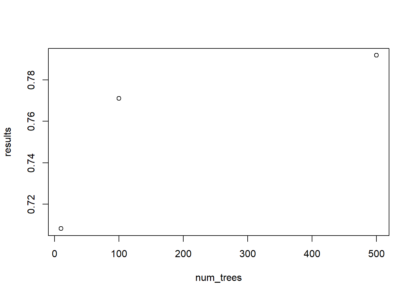
The results on the validation set clearly indicate that ntree = 500 outperforms the variants with fewer trees. We now want to fit the entire training data with this parameter setting. This entire part is quite important as many starting data scientists tend to forget this. Once you get the optimal parameter settings out of your validation set, you add the validation set to the training set. This ensures you use all avalaible data when building a model. More data often leads to more accurate predictions!
To have all the feasible data points, we stack train and val into one large dataframe, which we will call trainbig. We then use the same syntax as before on trainbig and test, but this time with the optimal parameter settings. The optimal ntree will be detected automatically, as this is useful for when you will be creating more complex scripts, later on in the course.
trainbig <- bind_rows(train, val)
optimal_ntree <- outcome[, 1][which.max(outcome[, 2])]

# fit
rFmodel <- randomForest(churn ~ ., data = trainbig, ntree = optimal_ntree)
# predict
predictions <- predict(rFmodel, test, type = "prob")[, 2]
# evaluate
AUC::auc(roc(predictions, test$churn))
## [1] 0.7973276The final estimation of our model’s AUC is 0.7847 (depends on your split, so can slightly deviate). Note how the test set performance slightly deviates from the performance on the validation set. This is partially explained by an increased number of training instances, but the measure is also dependent on how well the training and the test set match. This shows how different evaluation sets (which after all are selected randomly) can lead to different estimates of model performance.
Cross-validation
This was the inspiration behind cross-validation: rather than randomly doing the train/val/test split once, use different test sets and average out to make performance estimates more reliable. For instance, in the holdout set example above, we could use both sets once as a training and once as a test set, this would then be called 2-fold cross-validation. Instead of doing this 2 times, we could also do this three times: split the data into 3 equal parts, always use 2 parts as training and 1 part as testing. This would be an implementation of three-fold cross validation. However, the two most famous implementations in literature are 5-fold and 10 fold cross-validation. We will show you the latter: 10-fold cross-validation.
Rather than splitting the indices into two parts, we will now split them into ten equally large parts. Each fold then uses another part as test set (or validation depending on the application) (see theory).
# Randomly sample the indicators
allind <- sample(x = 1:nrow(basetable), size = nrow(basetable))

# create 10 equal chunks using these randomized indices
folds <- list()
for (i in 1:10) {
    indices <- allind[(round(length(allind) * (0.1 * (i - 1))) +
        1):round(length(allind) * (0.1 * i))]
    folds[[i]] <- indices  #store all indices per part in large object
}
This gives us 10 vectors of indices for each fold (folds[[1]], folds[[2]], …). By creating a new for loop, we can now create new train/test splits based on the splits in the folds list. Once the splits are made, we can repeat the same procedure as before. The only difference is the fact that this is not done 1 time, but 10 times. Note that, we should also create the all_aucs vector as we won’t be dealing with one, but multiple AUC estimates.
# Pre-assign a vector with length 10 Note that for
# memory-efficiency it is better to already lock 10 spots
# in the vector However, it is perfectly possible to just
# create a vector with no pre-defined length
all_aucs <- vector(length = 10)

# Start the loop to go over all folds
for (i in 1:10) {

    # block to test set
    ind <- folds[[i]]

    # Split in train/test
    train <- basetable[-ind, ]
    test <- basetable[ind, ]

    results <- vector()
    num_trees <- c(10, 100, 500)

    # fit (trees are set low for computational purposes)
    rFmodel <- randomForest(churn ~ ., data = train, ntree = 10)
    # predict
    predictions <- predict(rFmodel, test, type = "prob")[, 2]
    # evaluate and store
    all_aucs[i] <- AUC::auc(roc(predictions, test$churn))
}

# Let's plot the different AUCs
plot(all_aucs, type = "b")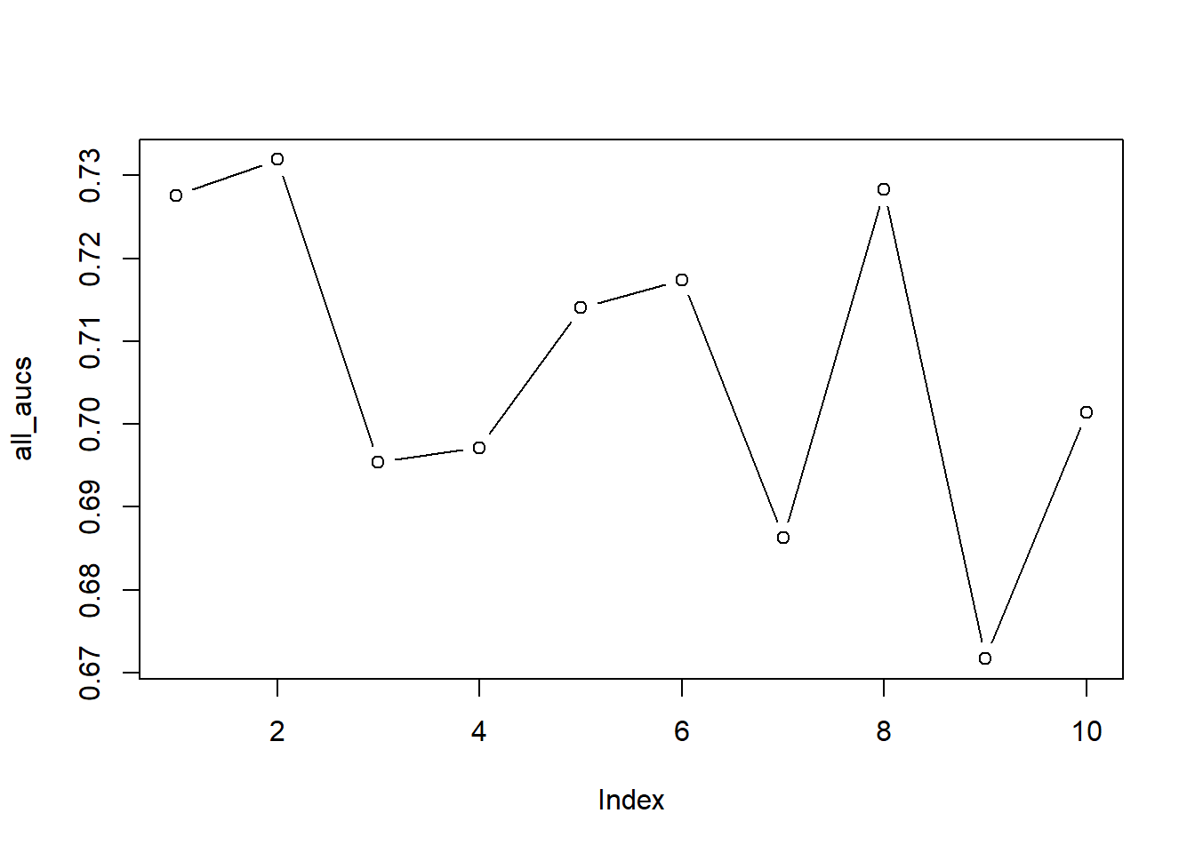
# Look at the mean and sd
mean(all_aucs)
## [1] 0.7071265sd(all_aucs)## [1] 0.01999184We observe that large deviations may occur between folds. If you look at the plot, you see the AUCs for all ten folds: you can clearly see that our estimates may have ranged from 0.68 to 0.75, which may have resulted in very different model evaluations.
Note how our single split was extremely optimistic.
LOOCV
LOOCV is a special case of k-fold cross validation, where the number of folds is equal to the number of observations. Below, we show how you could implement this by using the same syntax as used above. But be aware, as the method is highly suited for evaluating a single model, it is less suited for evaluating hyperparameters. Setting these parameters based on one observation is rather dangerous, as heavy overfitting to that value will occur. In fact, this is even infeasible, as one can not compute the ROC curve based on one validation or test observation. For our final performance estimate, we store the predictions per fold and only compute the AUC afterwards. When you run below’s block of code you can experience yourself why LOOCV is too slow for most real-life applications and is only perfroemd when the the data set is limited. Just imagine the run time across multiple parameter settings and algorithms!
#Create the folds manually
allind <- sample(x=1:nrow(basetable),size=nrow(basetable))
folds <- list()
for (i in 1:nrow(basetable)) {
  indices <- allind[(round(length(allind)*((1/nrow(basetable))*(i-1)))+1):round(length(allind)*((1/nrow(basetable))*i))]
  folds[[i]] <- indices #store all indices per part in large object
}


predictions <- vector()
true_outcome <- vector()

#Only take first 50 rows
#Replace 50 with nrow(basetable) to have actual LOOCV.

for (i in 1:50){
  cat('LOOCV run ', i, ' from the ', nrow(basetable), '\n')

  allind <- sample(x=1:nrow(basetable),size=nrow(basetable))
  #block the test indices
  ind <- folds[[i]]

  #actual subsetting
  train <- basetable[-ind,]
  test <- basetable[ind,]

  #fit
  rFmodel <- randomForest(churn ~ ., data = train, ntree = 10)
  #ntree set low for computational purposes
  #predict
  predictions <- c(predictions, predict(rFmodel,test,type="prob")[,2])
  true_outcome <- c(true_outcome, test$churn)

}
AUC::auc(roc(predictions,factor(true_outcome))) #
5x2cv
A popular variation to k-fold cross-validation is 5x2 cv. In this set-up, you repeat 2-fold cross-validation 5 times. The split is different each time, resulting in 10 unique training and test sets. Below is an example of how to efficiently code this.
# First make a partition function to create the 5x2cv folds
partition <- function(x, n = 1:nrow(x), p = 0.5, times = 5) {
    l <- list()
    for (i in 1:times) {

        ind_train <- sample(n, floor(p * length(n)), replace = FALSE)
        ind_test <- n[-ind_train]

        l[[i]] <- list(train = c(ind_train), test = c(ind_test))
    }
    l
}

# Make the folds
folds <- partition(x = basetable)

# Store in a different format to make the loop easier
folds2 <- train <- test <- list()
for (i in 1:length(folds)) {
    train[[i]] <- folds[[i]]$train
    test[[i]] <- folds[[i]]$test
}
folds2 <- c(train, test)

# Store your performance
perf <- numeric(length(folds2))

for (i in 1:length(folds2)) {

    cat(paste("Fold ", i), "\n")

    # Make the split
    train <- basetable[folds2[[i]], ]
    test <- basetable[-folds2[[i]], ]

    # fit
    rFmodel <- randomForest(churn ~ ., data = train, ntree = 10)
    # ntree set low for computational purposes predict
    predictions <- predict(rFmodel, test, type = "prob")[, 2]
    # evaluate and store
    perf[i] <- AUC::auc(roc(predictions, test$churn))
}
## Fold 1
## Fold 2
## Fold 3
## Fold 4
## Fold 5
## Fold 6
## Fold 7
## Fold 8
## Fold 9
## Fold 10# Let's plot the different AUCs
plot(perf, type = "b")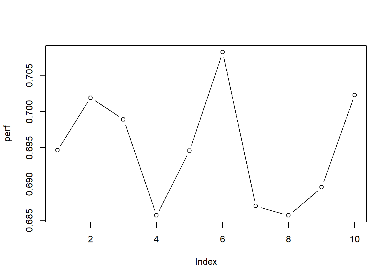
# Look at the mean and sd
mean(perf)
## [1] 0.6948437sd(perf)## [1] 0.007873238Note how the 5x2 cv method leads to more stable outcomes due to the larger test sets: the chance of a one-off easy/hard test set is becoming much smaller.
As a nice exercise, you can try to alter abive code if you should perform hyperparameter tuning. This would actually imply to use something called ‘nested cross-validation’.
Bootstrapping
A final set-up is the bootstrapping method. Rather than using each observation once, you allow observations to be used multiple times in the training set. The ones that are never sampled are used as unseen test set, leading to variation in the training and test sets. From the slides you should now that on average 1/3 of the observations are out-of-bag. Below you can find an example with 10 iterations.
# By setting a new unique seed, you ensure a different
# 'random' split
seeds <- c(123, 246, 91, 949, 9000, 1860, 1853, 1416, 515, 369)  #give 10 random values
all_aucs <- vector(length = length(seeds))

for (i in 1:length(seeds)) {
    set.seed(seeds[i])
    allind <- sample(x = 1:nrow(basetable), size = nrow(basetable),
        replace = TRUE)  # WITH replacement

    # block to get indices
    trainind <- allind[1:round(length(allind) * 0.5)]
    testind <- allind[!allind %in% trainind]  #get all indices which are not in training

    # actual subsetting
    train <- basetable[trainind, ]
    test <- basetable[testind, ]

    # do your parameter tuning here

    # fit on first set (train)
    rFmodel <- randomForest(churn ~ ., data = train, ntree = 10)
    # predict on second set (test)
    predictions <- predict(rFmodel, test, type = "prob")[, 2]
    # evaluate and store
    all_aucs[i] <- AUC::auc(roc(predictions, test$churn))
}

# Plot
plot(all_aucs, type = "b")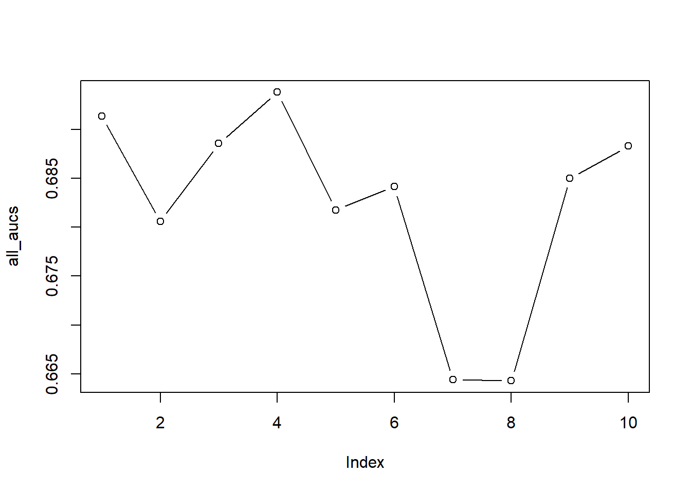
# Print
mean(all_aucs)
## [1] 0.6822259sd(all_aucs)## [1] 0.01025974# How many out of bag
nrow(test)/nrow(basetable)## [1] 0.3029301You might ask yourself the questions now whether there is no package available in R that allows you to make these splits. The answer is of course: Yes! The rsample package is a great package that contains a set of functions for different types of resampling methods. The package does not only make splits for cross-sectional data but also for times series and survival analysis. The two most important functions of this package are:
initial_split()which allows you to make a simple train/test split. You can set the proportion (prop) and also chose for a stratifief sample (strata).training()andtesting()should be used to extract the train and the test set.vfold_cv()which allows you to split the data into v folds of an equal size. The parameterVcontrols the number of partitions (normally referred to as k). You can also decide to repeat this procedure (repeats). There is again the option to create stratified folds. The training and test set per fold can be gathered using theanalysis()andassessment(). These terms are deliberately chosen to avoid conflict with the train and test splits made in theinitial_split()function.
We refer the reader to the package website for more information: https://rsample.tidymodels.org/index.html.
3.2 Bias-variance trade-off
Another vital concept in the data science is the bias-variance trade-off. If we oversimplify this concept, it boils down to models being too complex (high variance) or not complex enough (high bias). Consider our example above. We clearly observed that increasing the number of trees results in an increase of our random forest’s performance. This is because more trees represent a more complex model structure. Too few trees represent a less complex structure: the model underfits to the data. It is not capable of learning the more complex true underlying relation between independent and dependent variables. A quick conclusion could be to make models as complex as possible. This is, however, not necessarily true. If your model structure is too complex, your algorithm will learn the idiosyncrasies of the training data (i.e., overfit to the data). In that case, many small deviations will be learned that cannot be attributed to the included variables, which on its turn will lead to a model that does not generalise well and is highly unlikely in real life.
To demonstrate this, we will show three situations: one where we build our model not complex enough (underfitting), one where the model is specified with the optimal complexity, and one where model complexity is too high, resulting in overfitting to the data. To do so, we need to know the true underlying relationship. Therefore, we will use a synthetic example where we define the relationship ourselves. Note that we add some random noise to the model as well. This random noise represent the factors which we can not be aware of in real life, and to which the algorithm will overfit when model complexity is too high.
x <- c(-50:150)
y <- 3 + 2 * x^2 + rnorm(length(x), mean = 0, sd = 4000)
# true quadratic relationship + some random noise
plot(x, y)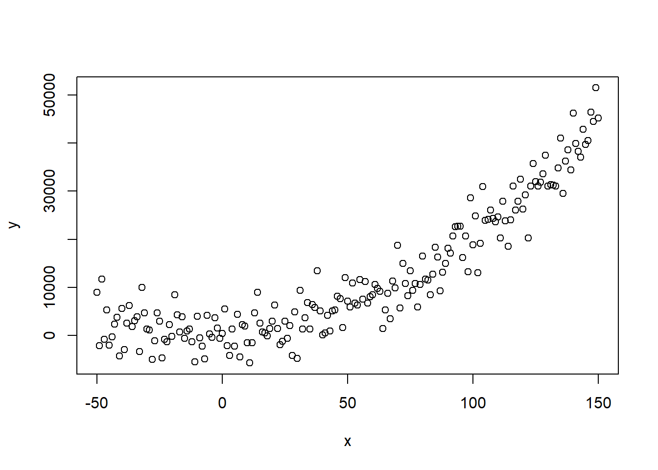
We can still clearly observe the true underlying relationship, but how will different models react to this input?
Let’s start with the least complex model specification: a linear relationship.
lin_model <- lm(y ~ x)
summary(lin_model)
##
## Call:
## lm(formula = y ~ x)
##
## Residuals:
## Min 1Q Median 3Q Max
## -13323.0 -5347.4 -699.8 4406.6 19623.5
##
## Coefficients:
## Estimate Std. Error t value Pr(>|t|)
## (Intercept) 1922.332 623.574 3.083 0.00234
## x 200.752 8.141 24.659 < 2e-16
##
## (Intercept) **
## x ***
## ---
## Signif. codes:
## 0 '***' 0.001 '**' 0.01 '*' 0.05 '.' 0.1 ' ' 1
##
## Residual standard error: 6697 on 199 degrees of freedom
## Multiple R-squared: 0.7534, Adjusted R-squared: 0.7522
## F-statistic: 608 on 1 and 199 DF, p-value: < 2.2e-16The model finds a significant positive relationship between predictor and response. Most people would be satisfied with this result, however, if we plot the relationship, we observe clearly that the true relationship is not represented by the modelled relationship: it is not complex enough.
predict_linear <- lin_model$coefficients[1] + lin_model$coefficients[2] *
    x
plot(x, y)
lines(x, predict_linear, col = "red")  #lines function plots over previous plot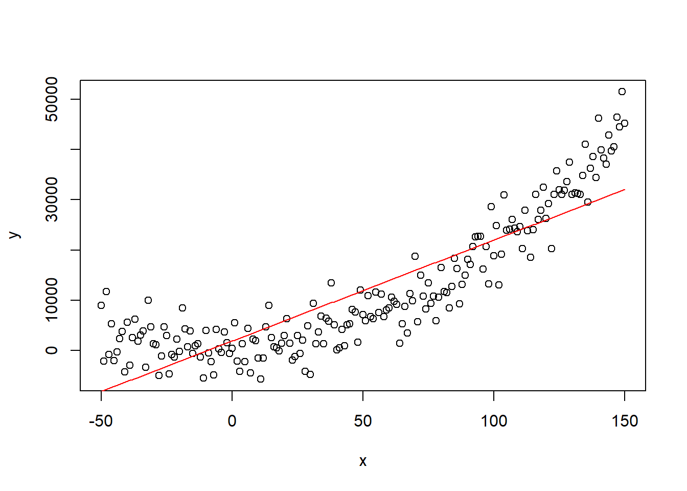
As a true data scientist you are not satisfied with this result and you decide to build a more complex model, so you build a complex fifth order polynomial model. To do so you create a new dataframe with some high powers of x.
df <- data.frame(x4 = x^4, x5 = x^5, y = y)
polynomial <- lm(y ~ ., df)
summary(polynomial)
##
## Call:
## lm(formula = y ~ ., data = df)
##
## Residuals:
## Min 1Q Median 3Q Max
## -10887.6 -2793.4 -124.2 2767.6 10980.3
##
## Coefficients:
## Estimate Std. Error t value
## (Intercept) 2.313e+03 3.912e+02 5.913
## x4 3.561e-04 2.312e-05 15.405
## x5 -1.853e-06 1.650e-07 -11.234
## Pr(>|t|)
## (Intercept) 1.45e-08 ***
## x4 < 2e-16 ***
## x5 < 2e-16 ***
## ---
## Signif. codes:
## 0 '***' 0.001 '**' 0.01 '*' 0.05 '.' 0.1 ' ' 1
##
## Residual standard error: 4153 on 198 degrees of freedom
## Multiple R-squared: 0.9057, Adjusted R-squared: 0.9047
## F-statistic: 950.5 on 2 and 198 DF, p-value: < 2.2e-16This seems pretty good, the R-squared has gone up and x4 and x5 are highly significant. However, when we plot the fitted relationship against the actual values, we observe a ‘wobbly curve’.
predict_poly <- predict(polynomial, df)
plot(x, y)
lines(x, predict_poly, col = "blue")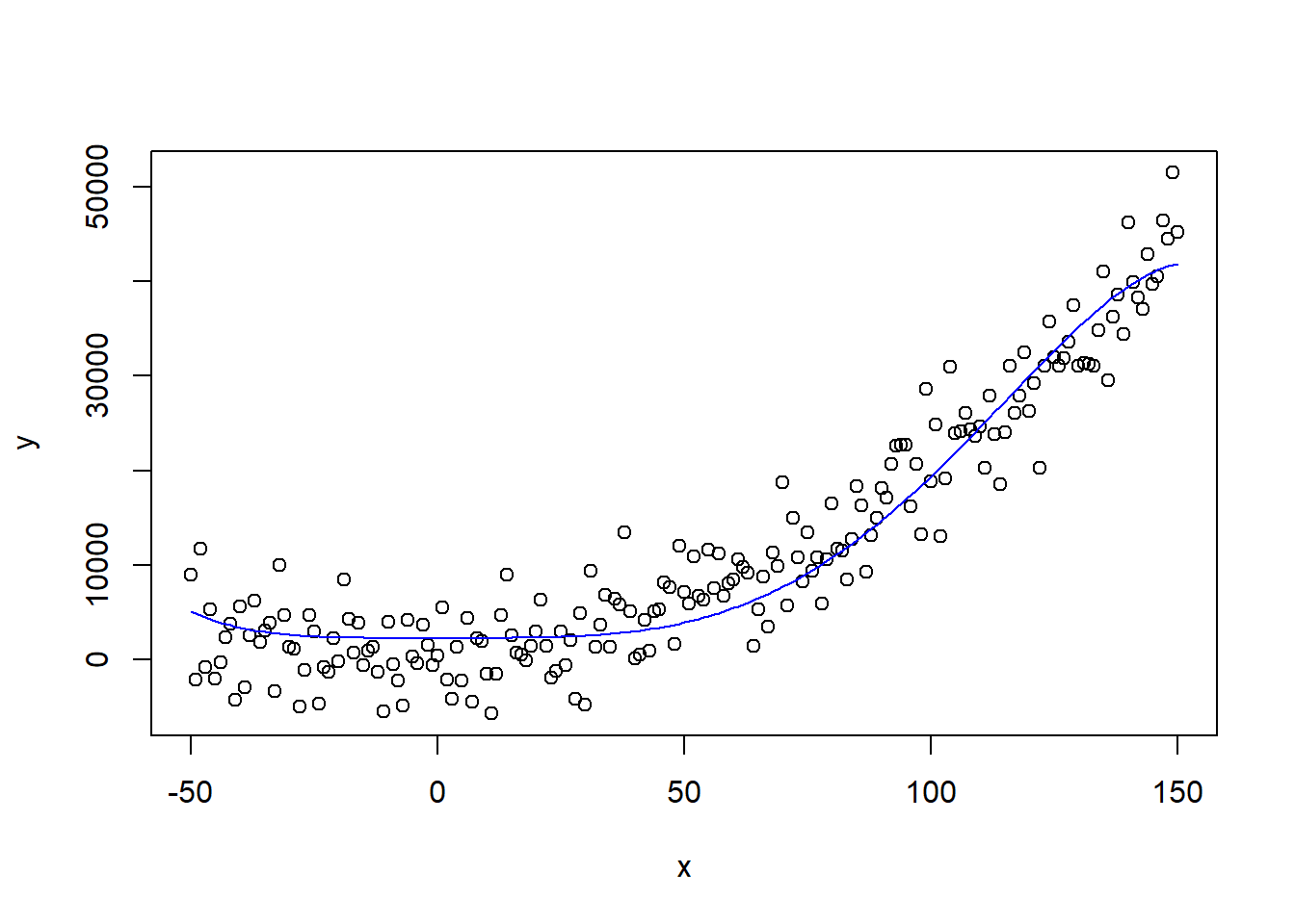
This is of course caused by the incorrect model formulation. When we create the correct model, we observe how the other algorithms overfit and underfit.
df$x2 <- x^2
quadratic <- lm(y ~ x2, df)
predict_quad <- predict(quadratic, df)
plot(x, y)
lines(x, predict_quad, lwd = 2)
lines(x, predict_poly, col = "blue")
lines(x, predict_linear, col = "red")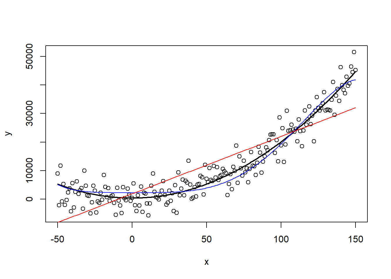
3.3 Performance measures
3.3.1 Regression
This was fairly easy as we know which underlying relationship is the correct one, but how do we do this is in real cases, where this of course is unknown? This is where model evaluation through performance measures comes into play. Let’s assume our x variable was a variable representing time and our y variable the profit during that period. As our profit follows a rather stable pattern, we want to predict the profit in the upcoming period (after x = 150). To do so, we of course are limited to the current data. How do we solve this?
Well, we can assume that the current underlying relaionship remains the same after so x = 150 (highly important assumption! this is not always true and can cause serious issues when assumed incorrectly!). We then try out different model specifications and the one which has the best performance on the hold out test set, is selected.
We will use the final 40 observations for testing, the final 80 to 40 observations for validation and the remainder for training:
df$x <- x  #add to make linear model of same format

# Make the test/val/train sets
test <- df[(length(x) - 39):length(x), ]
val <- df[(length(x) - 79):(length(x) - 40), ]
train <- df[1:(length(x) - 80), ]
We refit our three possible models on the training set.
linear <- lm(y ~ x, train)
quadratic <- lm(y ~ x2, train)
polynomial <- lm(y ~ x4 + x5, train)
Several measures exist to select the best method, when dealing with regression models. We will use a couple popular ones, but feel free to try out other ones as discussed in theory. Also, we will be coding the functions ourselves, but be aware of the fact that many packages implement these for you (e.g., yardstick). The R-squared can also be computed on the test set, as demonstrated, but is rather used as a goodness-of-fit of the training data and model specification (i.e., is the model not underfitting), while the RMSE, MAE, and MAPE measures are popular when dealing with predictive performance.
# Performance measures
RMSE <- function(true, predictions) {
    return(sqrt(mean((true - predictions)^2)))
}
MAE <- function(true, predictions) {
    return(mean(abs(true - predictions)))
}
MAPE <- function(true, predictions) {
    return(mean(abs(true - predictions)/true))
}
r_squared <- function(true, predictions) {
    return(1 - ((sum((true - predictions)^2))/sum((true - mean(true))^2)))
}

# all in one vector
performance_estimate <- function(true, predictions) {
    return(c(RMSE(true, predictions), MAE(true, predictions),
        MAPE(true, predictions), r_squared(true, predictions)))
}

# create predictions on validation set
predict_linear <- predict(linear, val)
predict_quad <- predict(quadratic, val)
predict_poly <- predict(polynomial, val)

# Print out
data.frame(measures = c("RMSE", "MAE", "MAPE", "Rsq"), linear = performance_estimate(val$y,
    predict_linear), quadratic = performance_estimate(val$y,
    predict_quad), polynomial = performance_estimate(val$y, predict_poly))
## measures linear quadratic
## 1 RMSE 10734.7178674 4054.2213575
## 2 MAE 9116.3213857 3278.1585710
## 3 MAPE 0.4778982 0.2615137
## 4 Rsq -1.8080429 0.5994678
## polynomial
## 1 22570.937393
## 2 19176.148298
## 3 1.157544
## 4 -11.414284We observe the quadratic model to be outperforming the other two models on all four performance measures. Note how the R-squared measure is the only one used which we are trying to maximize. The benefit of the MAPE and R-squared measures is that they are scaled between 0 and 1 (except for negative R-squared values which clearly indicates overfitting). The better performance is also observed when we plot the model’s predictions against their true values. While the quadratic model (green line) is the best model, we still observe a fair part of variance unexplained, this is why the R-squared is still far off a value of 1 and MAPE far off a value of 0. The polynomial model (blue line) tends to overestimate the dependent value and the linear model (red line) underestimates the values. Can you imagine how detrimental such models would be if actually deployed as profit forecasts?
plot(val$x, val$y)
lines(val$x, predict_quad)
lines(val$x, predict_poly, col = "blue")
lines(val$x, predict_linear, col = "red")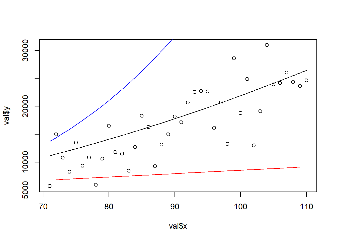
To have a final estimate of our model’s performance, we refit the preferred model (quadratic model) on our combined training and validation set and evaluate on the test set.
trainbig <- rbind(train, val)
final_model <- lm(y ~ x2, trainbig)
final_predictions <- predict(final_model, test)

# Print out
data.frame(measures = c("RMSE", "MAE", "MAPE", "Rsq"), performance = performance_estimate(test$y,
    final_predictions))
## measures performance
## 1 RMSE 4020.5795097
## 2 MAE 3258.0748934
## 3 MAPE 0.1095119
## 4 Rsq 0.7158729We observe the model to perform even better. This is good news, as this means that the model was able to learn the underlying relationship better due to the larger amount of data. This is also reflected when check the model’s coefficients, which are closer to their true values 3 and 2 (cf. supra).
summary(quadratic)##
## Call:
## lm(formula = y ~ x2, data = train)
##
## Residuals:
## Min 1Q Median 3Q Max
## -8069.3 -2221.1 230.6 2282.2 10142.0
##
## Coefficients:
## Estimate Std. Error t value Pr(>|t|)
## (Intercept) 216.2178 490.3223 0.441 0.66
## x2 2.1700 0.2651 8.186 3.44e-13
##
## (Intercept)
## x2 ***
## ---
## Signif. codes:
## 0 '***' 0.001 '**' 0.01 '*' 0.05 '.' 0.1 ' ' 1
##
## Residual standard error: 3778 on 119 degrees of freedom
## Multiple R-squared: 0.3602, Adjusted R-squared: 0.3549
## F-statistic: 67 on 1 and 119 DF, p-value: 3.445e-13summary(final_model)##
## Call:
## lm(formula = y ~ x2, data = trainbig)
##
## Residuals:
## Min 1Q Median 3Q Max
## -8580.1 -2507.8 206.5 2453.9 10271.6
##
## Coefficients:
## Estimate Std. Error t value Pr(>|t|)
## (Intercept) 258.85901 404.80477 0.639 0.523
## x2 2.05076 0.08861 23.144 <2e-16
##
## (Intercept)
## x2 ***
## ---
## Signif. codes:
## 0 '***' 0.001 '**' 0.01 '*' 0.05 '.' 0.1 ' ' 1
##
## Residual standard error: 3814 on 159 degrees of freedom
## Multiple R-squared: 0.7711, Adjusted R-squared: 0.7697
## F-statistic: 535.7 on 1 and 159 DF, p-value: < 2.2e-163.3.2 Classification
A somewhat similar approach can be followed when dealing with classification tasks. Also with classification tasks, several popular methods exist. Remember the example of the churn case? We will also be using that case for the discussion on classification measures. Once again, we will be calculating these measures ourselves, so that you understand what is happening, but be aware of the many packages do this for you.
With classification tasks, you can not simply measure the error, as all correct observations would have an error of 0 (0-0 or 1-1 in binary classification) and all incorrect observations would have an error of 1 (1-0 or 0-1). To handle this, are most popular performance measures based on a concept called the confusion matrix. The confusion matrix makes a cross tabulation of actual values and predicted values. Below is an example of such a cross tabulation.
# create training and test set
allind <- sample(x = 1:nrow(basetable), size = nrow(basetable))
ind <- allind[1:round(length(allind) * 0.5)]
train <- basetable[ind, ]
test <- basetable[-ind, ]

# Build a random forest model
rFmodel <- randomForest(churn ~ ., data = train, ntree = 10)

# Make predictions: default threshold = 0.50
predictions <- predict(rFmodel, test, type = "response")
labels <- test$churn

# Make cross tabulation true / predicted
table(labels, predictions)
## predictions
## labels 0 1
## 0 19978 125
## 1 708 58Ideally, we would want all observations to be positioned on the diagonal. However, this is often infeasible in most real life situations, as no model is perfect. So how should we interpret this model then? The model most often predicts the outcome to be non-churner (0). This is logical as there are much more non-churners in the training set than churners.
table(train$churn)##
## 0 1
## 20063 807But is this a behavior we desire? Out of the 763 churners in the test set, we only detect 45, this is only a small part, while detecting churners is the end goal of most retention campaigns. This already demonstrates the issues with the most popular classification performance measure: accuracy. Accuracy measures how often you were correct, without distinguishing the various categories. This causes are far from perfect model to have an accuracy of 0.96.
# Computation accuracy
sum(labels == predictions)/length(predictions)
## [1] 0.9600843So what should we do in order to detect these problems? Modelers have suggested different measures with special attention for the specific categories. The most renown ones are specificity and sensitivity (or recall). Sensitivity measures how many of the positives (churners) you detected and specificity measures how many negatives were detected.
# Sensitivity: True positives / all actual churners
table(labels, predictions)[2, 2]/sum(labels == 1)
## [1] 0.07571802# Specificity: True negatives / all actual non-churners
table(labels, predictions)[1, 1]/sum(labels == 0)## [1] 0.993782The issues we detected in our confusion matrix are nicely reflected in the sensitivity (very low, unable to detect all churners) and specificity scores (very high, almost all non-churners detected). The fact that there are much more negatives, results in the overall accuracy score being mainly determined by the specificity score.
While these new measures are already much better, they still suffer from one major downside: they are dependent on the used threshold. We used the default threshold, but what happens if we alter the threshold to, for instance, 0.05?
predictions_other_thres <- ifelse(predict(rFmodel, test, type = "prob")[,
    2] > 0.05, 1, 0) %>%
    as.factor()
table(labels, predictions_other_thres)
## predictions_other_thres
## labels 0 1
## 0 15884 4219
## 1 328 438While the used algorithm is the same, we get a completely different confusion matrix! This is also reflected in the performance measures based on the confusion matrix. While our accuracy and specificity have decreased, we are now actually able to detect more churners, as measured by the sensitivity measure.
# accuracy
sum(labels == predictions_other_thres)/length(predictions_other_thres)
## [1] 0.782117# Sensitivity
table(labels, predictions_other_thres)[2, 2]/sum(labels == 1)## [1] 0.5718016# Specificity
table(labels, predictions_other_thres)[1, 1]/sum(labels == 0)## [1] 0.7901308Of course you should alter your decision cut-off in order to detect an optimal number of would-be churners. However, this decision is based on your model, does not change the quality of your model! So how should we evaluate models if their performance depends heavily on the used treshold? The answer lays in cut-off independent performance measures.
The most popular cut-off independent measure is probably the AUC based on the ROC curve. The receiver operating characteristic curve is based on the ingenious idea to plot cut-off dependent measures (i.e., sensitivity and specificity) against different cut-offs, the AUC then calculates the integral below this curve resulting in a cut-off independent measure that values how good the model is at detecting both positives and negatives for each threshold. Many methods exist to do so, such as the AUC package used in the experimental set-up examples. We will , however, calculate a simplified ROC curve ourselves to show the reasoning behind it. However, when performing analysis yourselves, you can (and should!) use a package when you are asked to evaluate a model using the AUC measure.
# Create function that computes sensitivity and specificity
# against various thresholds
roc_point <- function(thres, predictions, labels) {
    pred <- ifelse(predictions > thres, 1, 0)
    # Sensitivity
    sens <- sum(labels == 1 & pred == 1)/sum(labels == 1)
    # Specificity
    spec <- sum(labels == 0 & pred == 0)/sum(labels == 0)
    return(c(sens, (1 - spec)))
}

# Create predictions
predictions <- predict(rFmodel, test, type = "prob")[, 2]
# Get true values
labels <- test$churn

# Apply function over range of thresholds
roc_curve <- sapply(seq(min(predictions), max(predictions), 0.01),
    function(x) roc_point(x, predictions, labels))

roc_curve <- data.frame(t(roc_curve))  #transpose for more easy plotting
roc_curve <- rbind(c(1, 1), roc_curve)  #add top right corner to complete graph
names(roc_curve) <- c("sensitivity", "1-specificy")
plot(roc_curve$`1-specificy`, roc_curve$sensitivity, type = "l",
    xlab = "1 - Specificity", ylab = "Sensitivity")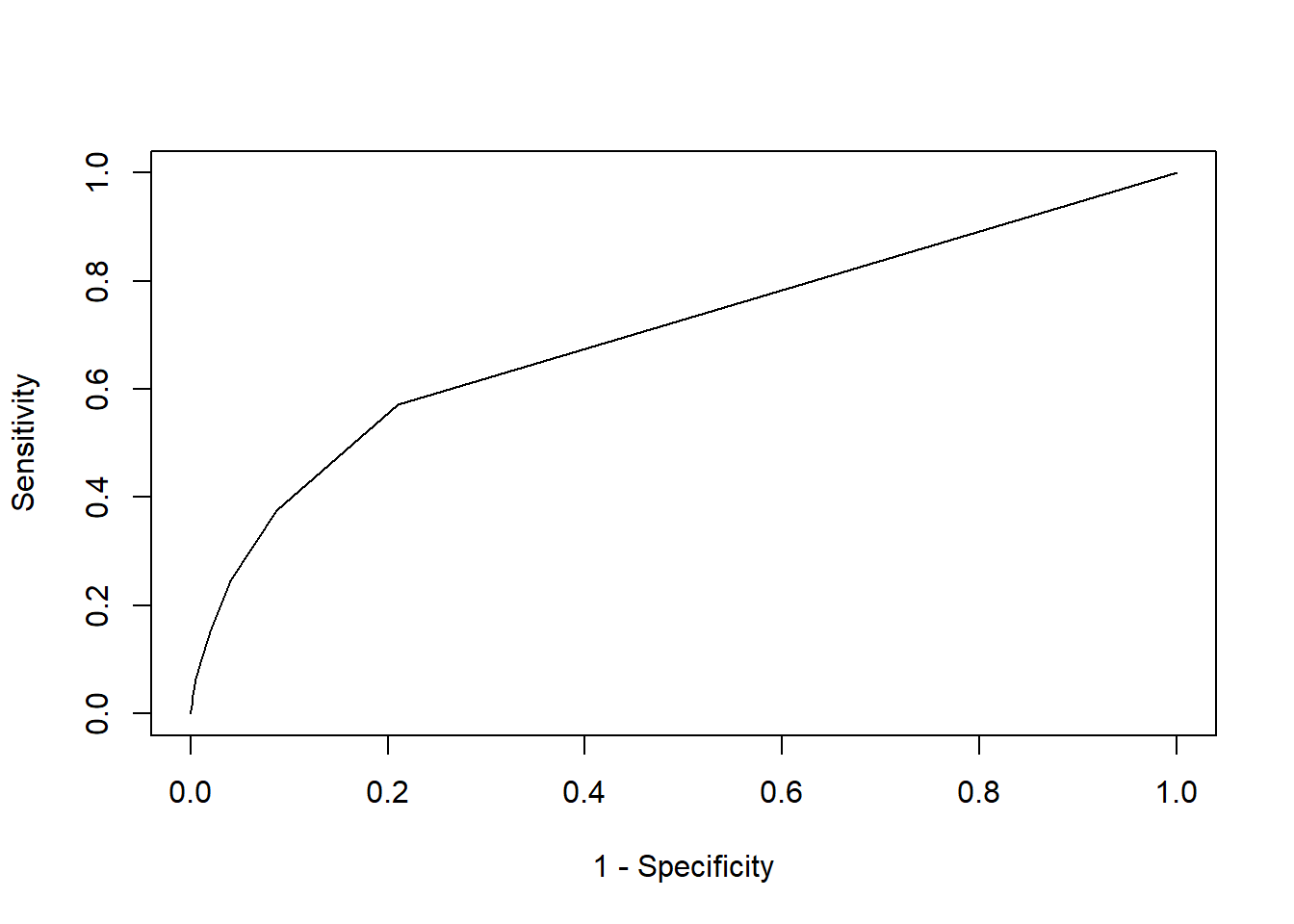
We nicely observe an ROC curve. The graph also displays how the model has much more difficulties in getting high sensitivity scors, while obtaining high specificity scores. Now how do we compute the AUC of this curve? Simply by calculating the area under the curve per step: the area of different rectangles is calculated by their base (=the deltas of 1-specifity) x height (= sensitivity).
# Order to roc curve on 1-spec and keep the unique values
roc_curve <- roc_curve %>%
    arrange(`1-specificy`) %>%
    distinct(`1-specificy`, .keep_all = TRUE)

# Calculate the delta for 1-specifity
roc_curve <- roc_curve %>%
    mutate(temp = c(`1-specificy`[-1], NA)) %>%
    mutate(delta = temp - `1-specificy`) %>%
    dplyr::select(-temp)

# calculate actual AUC
sum(roc_curve$delta * roc_curve$sensitivity, na.rm = TRUE)
## [1] 0.5139874This was a very simplified version of AUC computation, so we will likely have some rounding errors (notice how we have only 12 unique data points in roc_curve) when we compare with what the AUC package calculation gives :
# Load the package
p_load(AUC)

# Make a roc curve
plot(roc(predictions, labels), lwd = 2)

# Add our curve
lines(roc_curve$`1-specificy`, roc_curve$sensitivity, col = "red")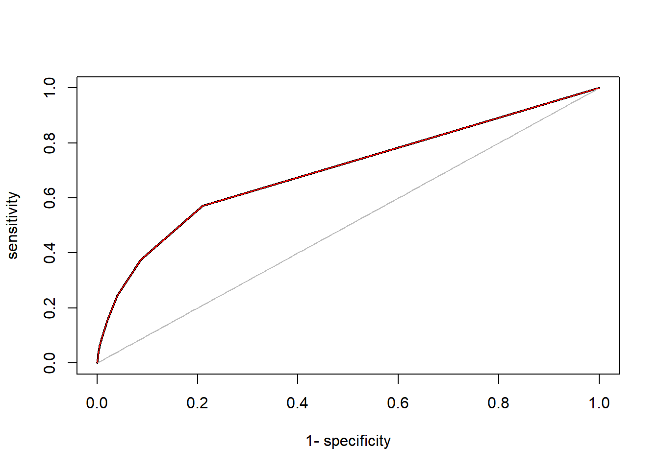
# As you can see they largely overlap# Now calculate the AUC
AUC::auc(roc(predictions, labels))## [1] 0.6995941The quick calculation of the area under the curve led to some rounding errors, which is why our AUC is deviating strongly from the ‘true’ value. However, when we inspect the curves, we see that they are virtually the same. The black curve seems to simply have used more data points (smaller sequence step size). When you calculate AUC and/or ROC, simply use the provided package (other good packages are yardstick, pROC and the godfather of classification performance packages ROCR), but make sure that you actually understand what is happening.
A final interesting measure we will be discussing is the top decile lift (TDL). This (and other lift measures) is especially interesting when you have a model which is not built to detect all categories (e.g., fingerprint recognition) but when you use the model to have more targeted actions (e.g., churn campaigns). When you have a retention campaign, you will only contact x% of your customers, the ones you think are most plausible to churn. If you would contact exactly 10% of your customer base, the top decile lift actually tells you how much better you would do than an informed campaign without a machine learning model. To understand this, it is important to realize that uninformed campaigns are also successful to a certain degree. When 5% of your customers churns, and you contact 100 customers, you will (on average) have contacted 5 customers that are actual churners. The idea behind lift is to check how much better your model is in detecting positives compared to this random success rate. Do note that while TDL in the 10% is the most common lift measure, you can also calculate other metrics such as the top 5% lift or top percentage lift.
# Calculate average random success rate (= churn rate)
random_rate <- sum(labels == 1)/length(labels)

# Calculate model's success rate in the top decile To do so
# order your labels in terms of your predictions and select
# the top 10%
top_decile <- labels[order(predictions, decreasing = TRUE)[1:round(0.1 *
    length(labels))]]
model_success <- sum(top_decile == 1)/length(top_decile)

# Top decile lift
model_success/random_rate
## [1] 3.811828Our model is more than 3 times as good in detecting churners when we contact 10% of our customer base when compared to a random model! But what about different contact rates? This is where the lift curve comes in, which displays the lift for different contact rates.
random_rate <- sum(labels == 1)/length(labels)

lift <- function(contact_rate, predictions, labels) {

    # Calculate the random state
    random_rate <- sum(labels == 1)/length(labels)

    # Calculate model's success rate in the top decile
    top_percent <- labels[order(predictions, decreasing = TRUE)[1:round(contact_rate *
        length(labels))]]
    model_success <- sum(top_percent == 1)/length(top_percent)

    liftv <- model_success/random_rate
    # Top decile lift
    return(liftv)
}

# Note that this curve calculates the lift for each contact
# rate and is cumulative Cumulative means that the lift
# always ranges from 0 to the contact level A noncumulative
# curve would calculate the lift per bucket (e.g., per
# bucket of 10) It is also possible to make this curve
# non-cumulative As an exercise you can do this for
# yourself.
lift_values <- sapply(seq(0.01, 1, 0.01), function(x) lift(x,
    predictions, labels))
plot(seq(0.01, 1, 0.01), lift_values, type = "l")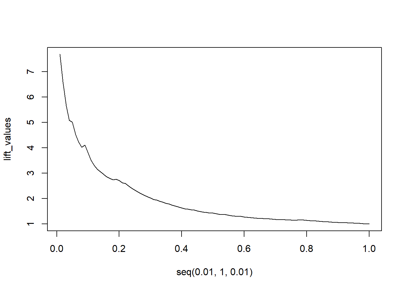
The model clearly outperforms a random model. Even for extremely high contact rates of 30%, we still see a lift rate of 2, meaning the model still is twice as good as randomly contacting people.
Of course, you can use a package to calculate the TDL and the lift curve. This can be done easily with the lift package.
p_load(lift)

# TDL in top 10%
TopDecileLift(predictions, labels)
## [1] 3.812# Lift curve Our curve had 100 buckets and was cumulative
plotLift(predictions, labels, cumulative = TRUE, n.buckets = 100)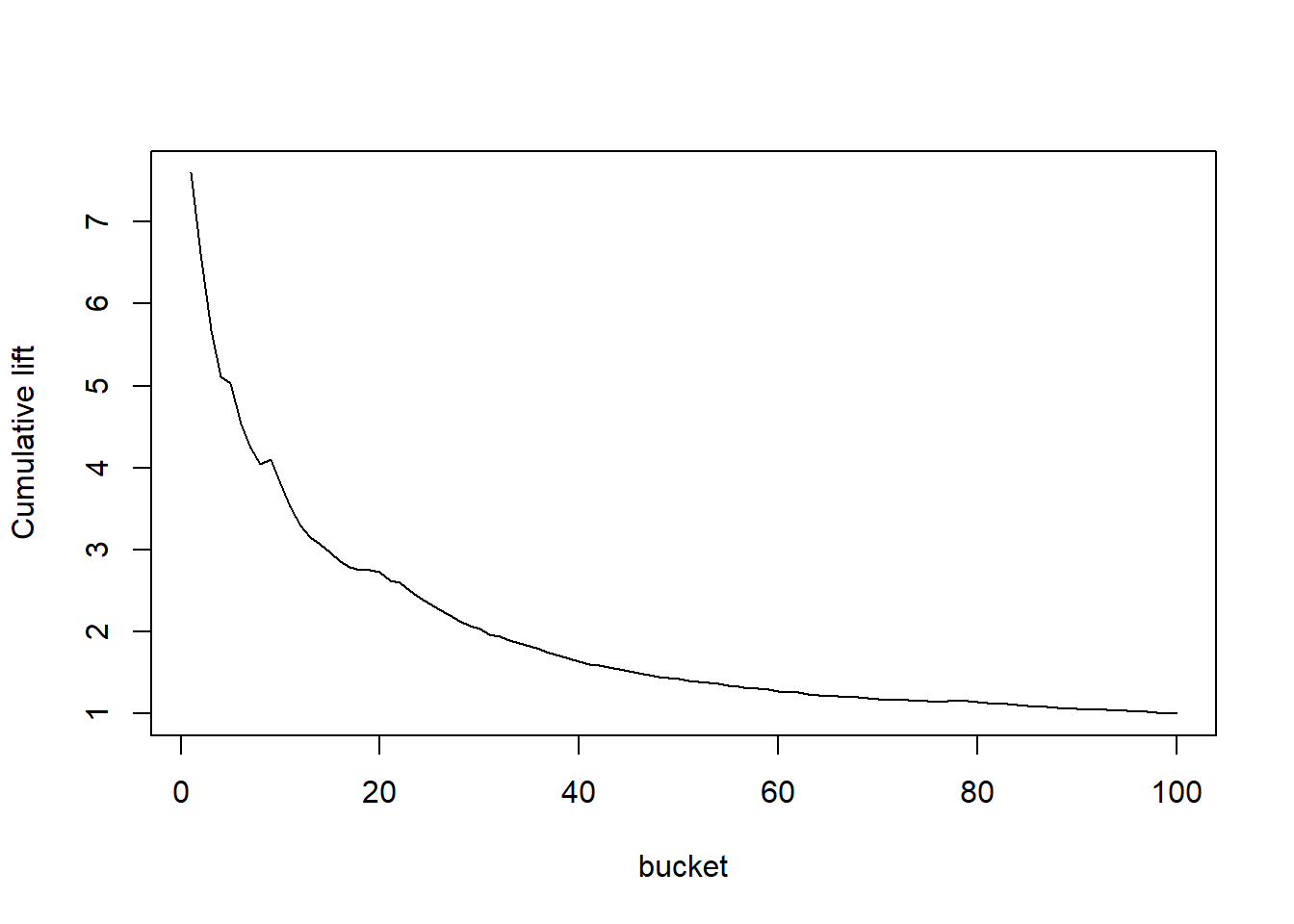
# The default is often 10 buckets
plotLift(predictions, labels, cumulative = TRUE, n.buckets = 10)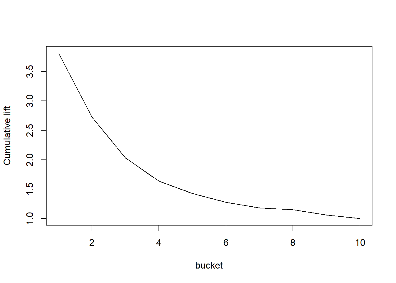
# A noncumulative curve is much bumpier
plotLift(predictions, labels, cumulative = FALSE, n.buckets = 10)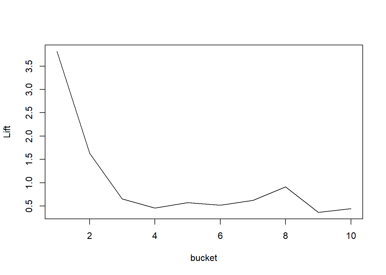
The other classification metrics like the accuracy ratio and the KS-distance can be easily calculated using the values of the ROC curve. The F1 measure and precision recall curves can be calculated using the ROCR or yardstick package.
3.4 Basic Analytical Models
In this final part, we will cover three major analytical models: linear regression, logistic regression, and decision trees.
3.4.1 Linear regression
Linear regression is the bread and butter of machine learning. The algorithm assumes a linear relationship between predictors and response. When dealing with two predictor variables, this can be formulated as \(y = \beta_0 + \beta_1 x_1 + \beta_2 x_2 + \varepsilon\). This means the model has to estimate three parameters: \(\beta_0, \beta_1, \beta_2\). These parameters are estimated in a way that the (quadratic) error term in the equation is minimized.
Because linear regression assumes an unflexible, fixed relationship between x and y, for which parameters need to be estimated, it is called a parametric model. Assumptions of parametric models are very important. Just think back about our example with a quadratic relationship: when simply assuming a linear relationship, our model achieved highly incorrect fit between x and y. This outlines the main issue with parametric models: when the assumed relationship between predictor and response reflects their true relationship, these models are highly performant. However, these assumed relationships often do not reflect the true relationship in real life. In real life, we often observe complex, nonlinear relationships.
Consider the assumed relationship below. After x = 30, the slope of the curve flattens out. The linear regression model will never be able to detect such a change in slope. The linear regression will, however, fit to the data on the assumption of a continuous linear relationship between predictor and response.
x <- seq(0, 50)
y <- ifelse(x < 30, x, 30 + 0.5 * (x - 30)) + rnorm(length(x),
    0, 3)
plot(x, y)
lines(x, ifelse(x < 30, x, 30 + 0.5 * (x - 30)))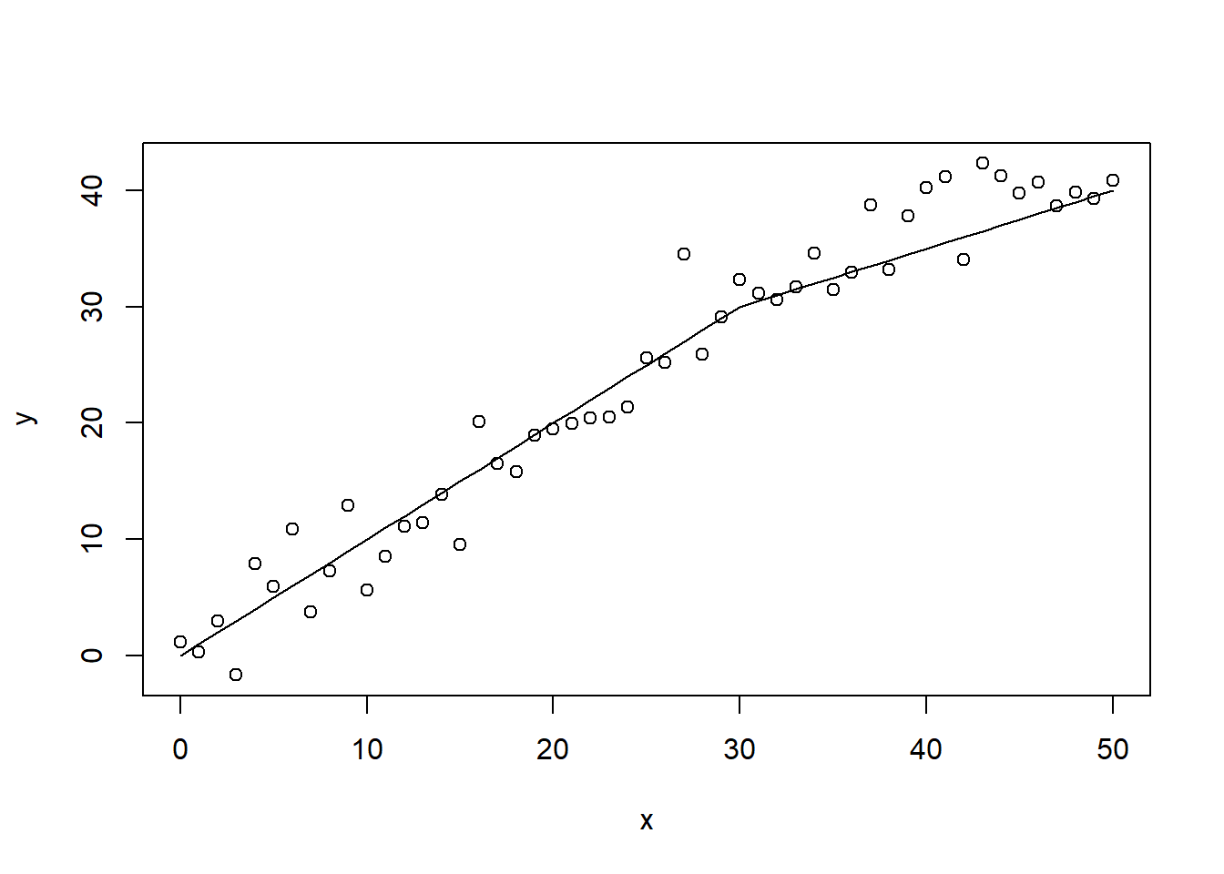
The model assumes a fixed \(\beta_1\) coefficient. The values \(\beta_0\) = -1.64 and \(\beta_1\) = 1.16 are the optimal OLS coefficients.
lin1 <- lm(x ~ y)
summary(lin1)
##
## Call:
## lm(formula = x ~ y)
##
## Residuals:
## Min 1Q Median 3Q Max
## -9.8402 -2.1276 -0.2356 1.7265 7.0686
##
## Coefficients:
## Estimate Std. Error t value Pr(>|t|)
## (Intercept) -0.18829 0.97899 -0.192 0.848
## y 1.07261 0.03624 29.599 <2e-16
##
## (Intercept)
## y ***
## ---
## Signif. codes:
## 0 '***' 0.001 '**' 0.01 '*' 0.05 '.' 0.1 ' ' 1
##
## Residual standard error: 3.456 on 49 degrees of freedom
## Multiple R-squared: 0.947, Adjusted R-squared: 0.946
## F-statistic: 876.1 on 1 and 49 DF, p-value: < 2.2e-16The linear regression model clearly results in a misfit here. However, on average, the error is not that large. The overall ‘acceptable error’, easy implementation, and highly interpretable model specification, causes the linear regression model to remain highly popular in many applications.
predict <- lin1$coefficients[1] + lin1$coefficients[2] * x
plot(x, y)
lines(x, ifelse(x < 30, x, 30 + 0.5 * (x - 30)))
lines(x, predict, col = "red")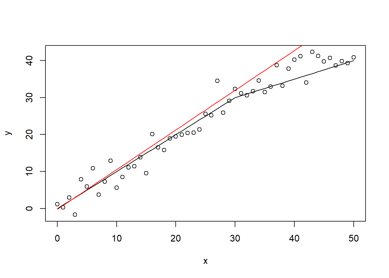
Consider following example: we have a dataset about Airbnb accomodations and various factors influencing the monthly demand, such as price per person, whether the host is a ‘superhost’, the location, etc. While all these variables are unlikely to display a linear relationship to the response variable, using a linear regression model we can predict on average 5 days incorrect of the monthly demand (limited to range 0-30 days). While this is not a spectacular model, we are able to make informed decisions based on this model: will demand be high or low? What measures should we take?.
airbnb <- read_csv("C:\\Users\\matbogae\\OneDrive - UGent\\PPA22\\PredictiveAnalytics\\Book_2022\\data codeBook_2022\\basetable_regression.csv")## New names:
## * `` -> ...1## Rows: 6862 Columns: 11## -- Column specification --------------------------
## Delimiter: ","
## dbl (11): ...1, host_id, accommodates, review_...##
## i Use `spec()` to retrieve the full column specification for this data.
## i Specify the column types or set `show_col_types = FALSE` to quiet this message.# remove index column
airbnb[, 1] <- NULL
# train test split
allind <- sample(x = 1:nrow(airbnb), size = nrow(airbnb))
ind <- allind[1:round(length(allind) * 0.5)]
train <- airbnb[ind, ]
test <- airbnb[-ind, ]
# Take a look at the data
airbnb %>%
glimpse()## Rows: 6,862
## Columns: 10
## $ host_id <dbl> 1, 1, 1, 1, 1, 0, 1~
## $ accommodates <dbl> 3, 2, 5, 2, 4, 3, 2~
## $ review_scores_rating <dbl> 97, 95, 98, 86, 97,~
## $ distance <dbl> 4.531863, 6.973741,~
## $ demand <dbl> 1.79, 1.38, 25.80, ~
## $ entire_home <dbl> 1, 0, 1, 0, 1, 0, 0~
## $ washer_drier <dbl> 1, 1, 1, 1, 0, 0, 1~
## $ superhost <dbl> 1, 1, 0, 1, 0, 1, 1~
## $ response <dbl> 86, 100, 60, 83, 10~
## $ price_pp <dbl> 98.33333, 54.50000,~# Look for missing values
colSums(is.na(airbnb))## host_id accommodates
## 0 0
## review_scores_rating distance
## 1292 0
## demand entire_home
## 0 0
## washer_drier superhost
## 0 0
## response price_pp
## 869 0# Handle missing values
train$review_scores_rating <- ifelse(is.na(train$review_scores_rating),
median(train$review_scores_rating, na.rm = TRUE), train$review_scores_rating)
test$review_scores_rating <- ifelse(is.na(test$review_scores_rating),
median(train$review_scores_rating, na.rm = TRUE), test$review_scores_rating)
train$response <- ifelse(is.na(train$response), median(train$response,
na.rm = TRUE), train$response)
test$response <- ifelse(is.na(test$response), median(train$response,
na.rm = TRUE), test$response)
# Build a linear regression model
lin_airbnb <- lm(demand ~ ., train)
predicted_demand <- predict(lin_airbnb, test)
RMSE(test$demand, predicted_demand) #Re-use function as defined above to evaluate## [1] 5.466273A random model would assume all demand to be equal. The RMSE measure below indicates that our model performs only slightly better than a random model.
RMSE(test$demand, rep(mean(train$demand, na.rm = TRUE), nrow(test)))## [1] 5.647598When we inspect the model’s coefficients, we observe the coefficient of host_id and response variable to be insignificant. This is problematic, as the model uses hese terms to predict demand. This while response has no impact! To overcome this, 2 popular methods have been proposed: (1) stepwise variable selection and (2) regularization. A number of issues arise with the usage of stepwise variable selection (https://towardsdatascience.com/stopping-stepwise-why-stepwise-selection-is-bad-and-what-you-should-use-instead-90818b3f52df for a more elaborate take on that statement). We will shortly cover stepwise variable selection, but remember the downsides that are linked to this approach.
summary(lin_airbnb)##
## Call:
## lm(formula = demand ~ ., data = train)
##
## Residuals:
## Min 1Q Median 3Q Max
## -10.779 -3.521 -1.650 1.910 27.676
##
## Coefficients:
## Estimate Std. Error
## (Intercept) 12.4491704 1.7379258
## host_id 0.4086691 0.1918584
## accommodates -0.4266254 0.0548386
## review_scores_rating -0.0994547 0.0157651
## distance 0.2296981 0.0360469
## entire_home 1.2275841 0.2147551
## washer_drier -0.5085887 0.2117872
## superhost 2.2834934 0.2009903
## response 0.0092476 0.0093394
## price_pp -0.0015552 0.0008388
## t value Pr(>|t|)
## (Intercept) 7.163 9.60e-13 ***
## host_id 2.130 0.0332 *
## accommodates -7.780 9.56e-15 ***
## review_scores_rating -6.309 3.18e-10 ***
## distance 6.372 2.11e-10 ***
## entire_home 5.716 1.18e-08 ***
## washer_drier -2.401 0.0164 *
## superhost 11.361 < 2e-16 ***
## response 0.990 0.3222
## price_pp -1.854 0.0638 .
## ---
## Signif. codes:
## 0 '***' 0.001 '**' 0.01 '*' 0.05 '.' 0.1 ' ' 1
##
## Residual standard error: 5.495 on 3421 degrees of freedom
## Multiple R-squared: 0.08195, Adjusted R-squared: 0.07954
## F-statistic: 33.93 on 9 and 3421 DF, p-value: < 2.2e-16Stepwise
# You can use the step function of MASS package
p_load(MASS)

# Input the regression model in the stepAIC function
lm_forward <- stepAIC(object = lin_airbnb, direction = "forward")
## Start: AIC=11701.18
## demand ~ host_id + accommodates + review_scores_rating + distance +
## entire_home + washer_drier + superhost + response + price_pplm_backward <- stepAIC(object = lin_airbnb, direction = "backward")## Start: AIC=11701.18
## demand ~ host_id + accommodates + review_scores_rating + distance +
## entire_home + washer_drier + superhost + response + price_pp
##
## Df Sum of Sq RSS AIC
## - response 1 29.6 103310 11700
## <none> 103281 11701
## - price_pp 1 103.8 103385 11703
## - host_id 1 137.0 103418 11704
## - washer_drier 1 174.1 103455 11705
## - entire_home 1 986.5 104267 11732
## - review_scores_rating 1 1201.5 104482 11739
## - distance 1 1225.9 104507 11740
## - accommodates 1 1827.2 105108 11759
## - superhost 1 3896.9 107178 11826
##
## Step: AIC=11700.16
## demand ~ host_id + accommodates + review_scores_rating + distance +
## entire_home + washer_drier + superhost + price_pp
##
## Df Sum of Sq RSS AIC
## <none> 103310 11700
## - price_pp 1 103.2 103414 11702
## - host_id 1 129.4 103440 11702
## - washer_drier 1 173.7 103484 11704
## - entire_home 1 992.7 104303 11731
## - review_scores_rating 1 1198.2 104509 11738
## - distance 1 1278.3 104589 11740
## - accommodates 1 1834.3 105145 11758
## - superhost 1 4067.7 107378 11831lm_both <- stepAIC(object = lin_airbnb, direction = "both")## Start: AIC=11701.18
## demand ~ host_id + accommodates + review_scores_rating + distance +
## entire_home + washer_drier + superhost + response + price_pp
##
## Df Sum of Sq RSS AIC
## - response 1 29.6 103310 11700
## <none> 103281 11701
## - price_pp 1 103.8 103385 11703
## - host_id 1 137.0 103418 11704
## - washer_drier 1 174.1 103455 11705
## - entire_home 1 986.5 104267 11732
## - review_scores_rating 1 1201.5 104482 11739
## - distance 1 1225.9 104507 11740
## - accommodates 1 1827.2 105108 11759
## - superhost 1 3896.9 107178 11826
##
## Step: AIC=11700.16
## demand ~ host_id + accommodates + review_scores_rating + distance +
## entire_home + washer_drier + superhost + price_pp
##
## Df Sum of Sq RSS AIC
## <none> 103310 11700
## + response 1 29.6 103281 11701
## - price_pp 1 103.2 103414 11702
## - host_id 1 129.4 103440 11702
## - washer_drier 1 173.7 103484 11704
## - entire_home 1 992.7 104303 11731
## - review_scores_rating 1 1198.2 104509 11738
## - distance 1 1278.3 104589 11740
## - accommodates 1 1834.3 105145 11758
## - superhost 1 4067.7 107378 11831# Evaluate performance
RMSE(test$demand, predict(lm_forward, test))## [1] 5.466273RMSE(test$demand, predict(lm_backward, test))## [1] 5.46599RMSE(test$demand, predict(lm_both, test))## [1] 5.46599Regularization
Regularization works with ingeneous system of a penalty term. This term is added to the general loss function (i.e., the error). The penalty consists of a weighted sum of the coefficient terms. This automatically sets coefficients equal to zero when their value is lower than the reduction in error term. Several implementations exist: L1-regularization (LASSO), L2-regularization, and elastic nets, as described in the theory slides. A crucial parameter is lambda as this parameter determines the relative importance of the penalty term (i.e., slight regularization or heavy regularization).
To implement regularized regression, we will use the glmnet package, as the default lm() function does not support this. Note how this package masks the auc function, which is why consequently notate the auc function as AUC::auc. glmnet does not use the default formula notation, so we need to adjust our dataset to data.matrix format. We also rename our training set to train big and create a train/val split to validate the optimal value of lambda.
Especially important is the alpha parameter or the elastic net mixing parameter. Remember: elastic net is a combination of L1 and L2 regularization. This means that L1 and L2 are extreme cases where alpha is equal to 1 (L1) or 0 (L2). By default alpha = 1, so L1 or LASSO.
Note that the glmnet function scales the coefficients by default, so there is no need to scale your variables upfront.
p_load(glmnet)

# Make a trainbig and then split into a smaller train and
# val set
trainbig <- train

allind <- sample(x = 1:nrow(trainbig), size = nrow(trainbig))
trainind <- allind[1:round(length(allind) * 0.5)]
valind <- allind[(round(length(allind) * (0.5)) + 1):length(allind)]
train <- trainbig[trainind, ]
val <- trainbig[valind, ]

# Separate the y variable because matrix notation is not
# allowed
y_train <- train$demand
y_val <- val$demand
y_test <- test$demand
y_trainbig <- trainbig$demand

train$demand <- val$demand <- test$demand <- trainbig$demand <- NULL

# LASSO regression: fit on training set
lasso_airbnb <- glmnet(x = data.matrix(train), y = y_train, alpha = 1)
We have now fitted the LASSO model for various lambdas on the training set. To see how the various coefficients shrink according to the regularization parameter lambda, we can plot following graph. Each colored line represents the coefficient value at different lambdas. We can clearly observe that larger lambdas lead to almost all coefficients set equal to zero.
plot(lasso_airbnb, xvar = "lambda")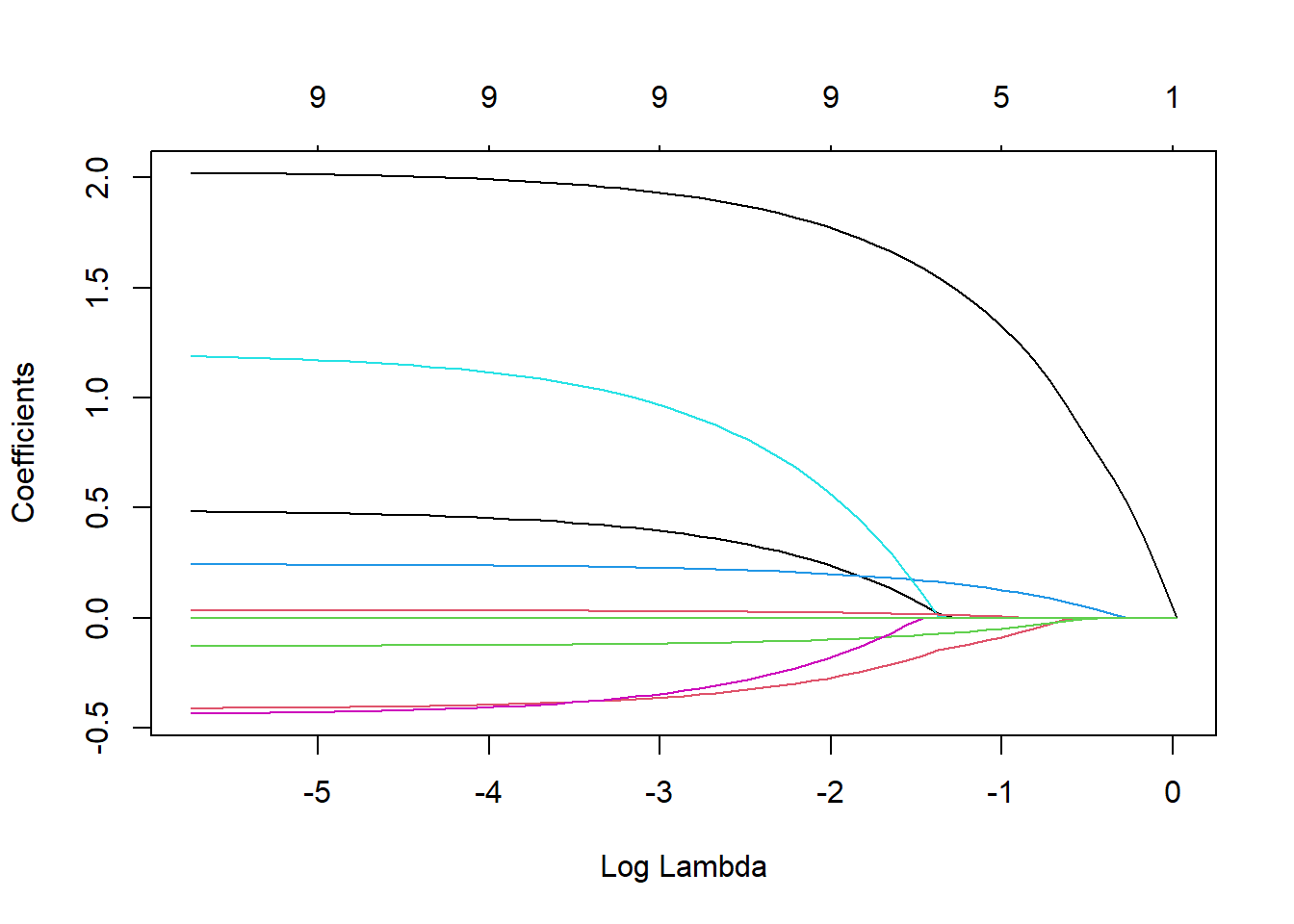
The above graph shows you that it is utterly important to tune lambda. We can do this in a similar approach as the one used for setting ntree in the random forest model. We are however dealing with regression, so we will use the RMSE as objective value. We will iterate over all possible values of lambda (automatically created when fitting the glmnet), we use the s parameter in the prediction function to alter the value of lambda. Note that we do not need to refit the model for each parameter setting (as opposed optimizing ntree for our random forest). This makes lambda parameter tuning extremely fast. In the plot we can clearly observe that our predictive performance improves with very high values of lambda.
rmse_store <- vector(length = length(lasso_airbnb$lambda))

for (i in 1:length(lasso_airbnb$lambda)) {
    predglmnet <- predict(lasso_airbnb, newx = data.matrix(val),
        type = "response", s = lasso_airbnb$lambda[i])
    rmse_store[i] <- RMSE(predglmnet, y_val)
}

# Let's determine the optimal lambda value
plot(1:length(lasso_airbnb$lambda), rmse_store, type = "b")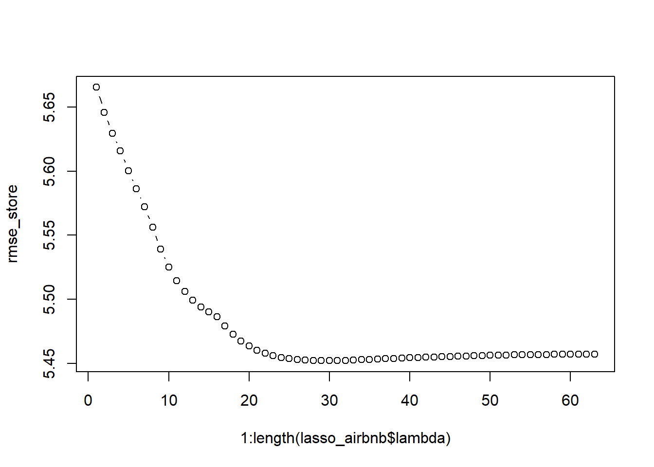
We automatically derive the optimal lambda setting as the one that minimizes the RMSE. Try, as a home exercise, to create the same methodology for an elastic net and ridge regression (alpha parameter!).
optimal_lam <- lasso_airbnb$lambda[which.min(rmse_store)]

# Now that we know the optimal lambda we can fit the model
# on trainbig.
final_lin <- glmnet(x = data.matrix(trainbig), y = y_trainbig)

# We then use that model with the optimal lambda.
pred_lasso <- predict(final_lin, newx = data.matrix(test), type = "response",
    s = optimal_lam)

# Finally we assess the performance of the model
RMSE(pred_lasso, y_test)
## [1] 5.4610633.4.2 Logistic regression
An important extension to linear regression is logistic regression. This basically is a linear regression that uses the logit function as an activation function. The activation function ensures that the output of the model lays between 0 and 1 (i.e., being probabilities). Otherwise, many classifier models would give non-sensical outputs.
The close alignment between linear regression and logistic regression ensures that we can follow a similar approach. The glmnet package also facilitates this type of model, we just have to specify that we are using a binomial (binary) response variable. We will be modelling the data from the above used churn case, but with a to-be optimized ridge regression model this time, rather than a random forest model.
#Let's use the churn example again

#glmnet needs numeric input rather than factor!
basetable$churn <- as.numeric(as.character(basetable$churn))

#Start with train/val/test splitting
allind <- sample(x=1:nrow(basetable),size=nrow(basetable))
trainind <- allind[1:round(length(allind)/3)]
valind <- allind[(round(length(allind)/3)+1):round(length(allind)*(2/3))]
testind <- allind[(round(length(allind)*(2/3))+1):length(allind)]
train <- basetable[trainind,]
val <- basetable[valind,]
test <- basetable[testind,]

trainbig <- rbind(train, val)

y_train <- train$churn
y_val <- val$churn
y_test <- test$churn
y_trainbig <- trainbig$churn

train$churn <- val$churn <- test$churn <- trainbig$churn <-  NULL

#LASSO regression: fit on training set
ridge <- glmnet(x = data.matrix(train),
                y = y_train,
                alpha = 0, #alpha = 0 to ensure ridge regression model
family = 'binomial') plot(ridge, xvar = "lambda")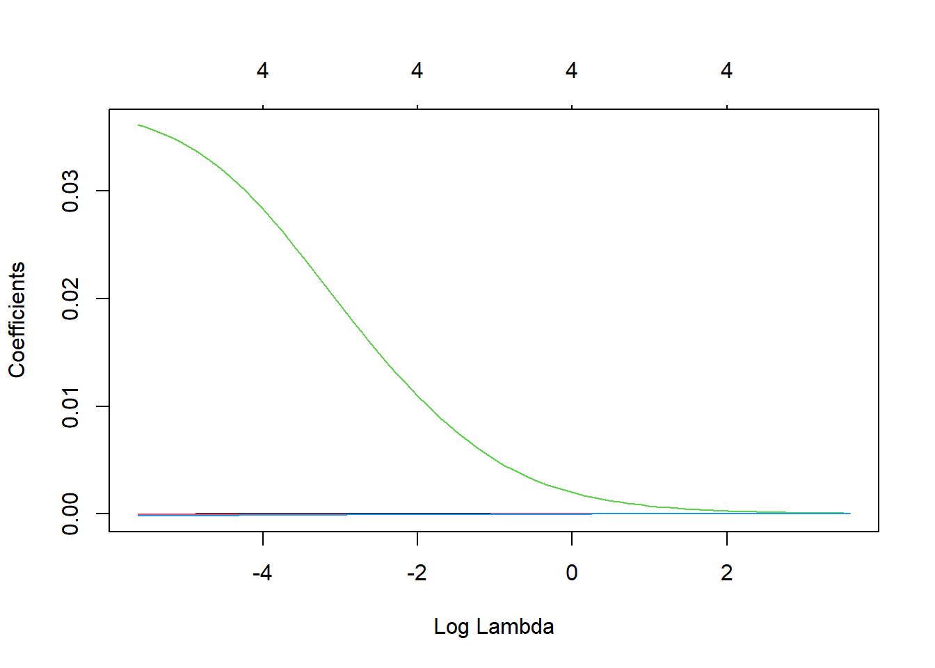
One variable is clearly very important, as its value remains positive for very high lambda values. We now optimize lambda on the validation set in terms of AUC.
auc_store <- vector()

for (i in 1:length(ridge$lambda)) {
    predglmnet <- as.numeric(predict(ridge, newx = data.matrix(val),
        type = "response", s = ridge$lambda[i]))
    auc_store[i] <- AUC::auc(roc(predglmnet, factor(y_val)))  #roc needs factor true values
}

# Let's determine the optimal lambda value
plot(1:length(ridge$lambda), auc_store, type = "b")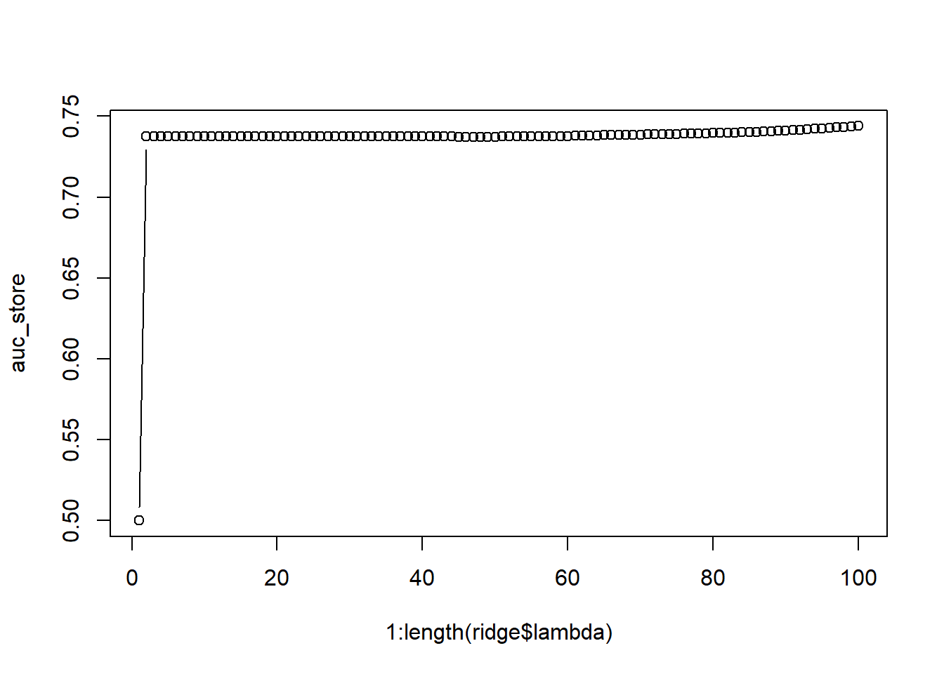
The best performance is obtained with very low values of lambda (end of the graph) This is because we only included the four most important variables. For extremely high values of lambda, the model even puts the coefficients of those highly predictive variables equal to zero.
(optimal_lam <- ridge$lambda[which.max(auc_store)])## [1] 0.003641277# Now that we know the optimal lambda we can fit the model
# on trainbig.
final_ridge <- glmnet(x = data.matrix(trainbig), y = y_trainbig,
alpha = 0)
# We then use that model with the optimal lambda
pred_ridge <- predict(final_ridge, newx = data.matrix(test),
type = "response", s = optimal_lam)
# Finally we assess the performance of the model
AUC::auc(roc(pred_ridge, as.factor(y_test)))## [1] 0.7131695Optimal performance is obtained a the lowest possible value of lambda (virtually no regularization). The lower performance compared to the random forest model also indicates that the assumed linear relationship between predictor and response is not complex enough to mimic the real life relationship and that our model is underfitting.
3.4.3 Decision trees
Many predictive models are based on the reasoning behind regression models (even deep learning models!), often with an adjustment to the assumed relationship between predictor and response. However, an entire group of machine learning models uses a completely different reasoning: decision trees. Rather than trying to find a function that defines \(y=f(x)\), they search for decision splits which ensure an adequate split between the categories. These splits are based on an impurity measure (see theory). However, if trees would just reduce impurity to the infinite, they would become too complex (= too many branches), and overfit to the data (similar to non-zero coefficients in regression models). Where regression handles this by use of a regularization penalty, decision trees use the cost complexity parameter, which can also be seen as a penalty term added to the impurity function. This makes this cost complexity parameter highly important. Therefore, we will tune it in a similar way as was done with lambda.
To implement simple descision trees, we will use the R package rpart, which implements CART trees. For this exercise, we will use a limited basetable of the newspaper publishing company. The data is already split into BasetableTRAIN, BasetableTRAINbig, BasetableVAL, BasetableTEST.
# Load the data
load("C:\\Users\\matbogae\\OneDrive - UGent\\PPA22\\PredictiveAnalytics\\Book_2022\\data codeBook_2022\\TrainValTest.Rdata")

# Take a glimpse at training set
BasetableTRAIN %>%
    glimpse()
## Rows: 707
## Columns: 7
## $ TotalDiscount <dbl> 22.79579, 0.00000~
## $ TotalPrice <dbl> 114.40, 972.00, 9~
## $ TotalCredit <dbl> 0.000, 0.000, 0.0~
## $ PaymentType_DD <dbl> 0, 0, 0, 0, 0, 0,~
## $ PaymentStatus_Not.Paid <dbl> 0, 0, 0, 0, 0, 0,~
## $ Frequency <dbl> 4, 4, 5, 4, 1, 5,~
## $ Recency <dbl> 295, 64, 341, 39,~table(yTRAIN)## yTRAIN
## 0 1
## 666 41# Load the rpart package
p_load(rpart)
# Estimate a tree model Make sure that your dependent
# variable is a factor
tree <- rpart(yTRAIN ~ ., BasetableTRAIN)
# We can also visualize the tree:
par(xpd = TRUE)
plot(tree, compress = TRUE)
text(tree, use.n = TRUE)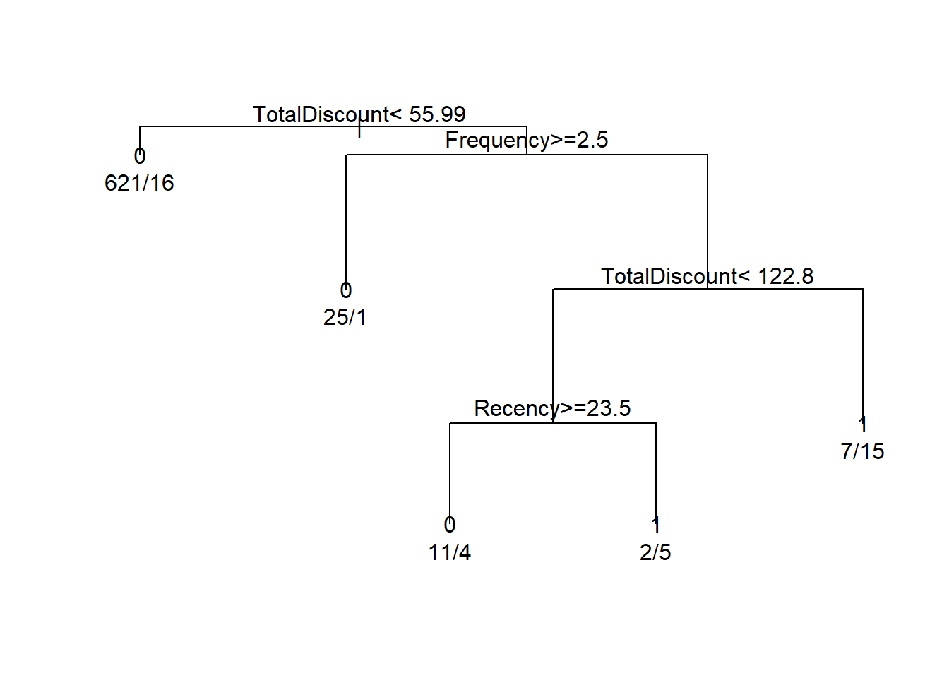
# Or more fancy
p_load(rpart.plot)
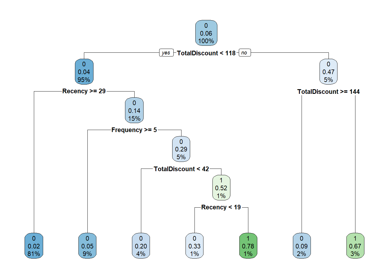
rpart.plot(tree)
How to interpret the tree? The first split is whether TotalDiscount < 109.9. If yes go to the left, otherwise go to the right. If we go to the right we encounter the same variable but now another split is used: TotalDiscount >= 146.6. If yes, go to the left. If no, go to the right. The numbers can be interpreted as follows:
-the top number is the predicted label (0 or 1),
-the second number is the predicted probability,
-and the third number the percentage of observations in this node.
We will focus on the tuning of the cost-complexity parameter. This can be done by the use of the control parameter cp (default = 0.01). Just observe how the different parameter settings influence the model.
# Estimate a tree model
tree <- rpart(as.factor(yTRAIN) ~ ., BasetableTRAIN, control = rpart.control(cp = 0.05))

# We can also visualize the tree:
rpart.plot(tree)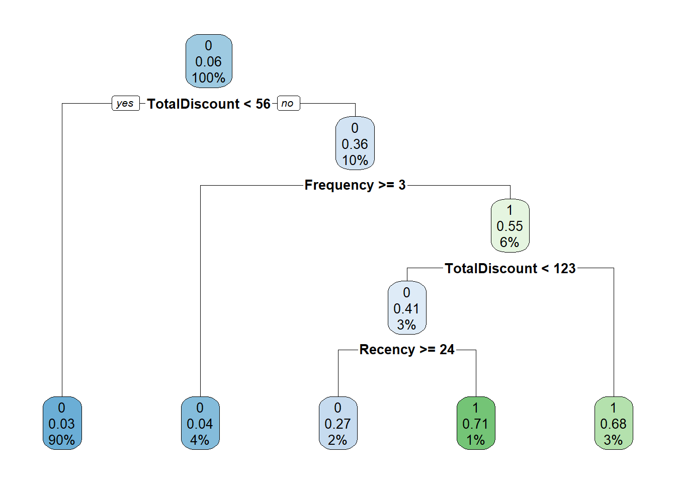
# Estimate a tree model
tree <- rpart(yTRAIN ~ ., BasetableTRAIN, control = rpart.control(cp = 0.001))

# We can also visualize the tree:
rpart.plot(tree)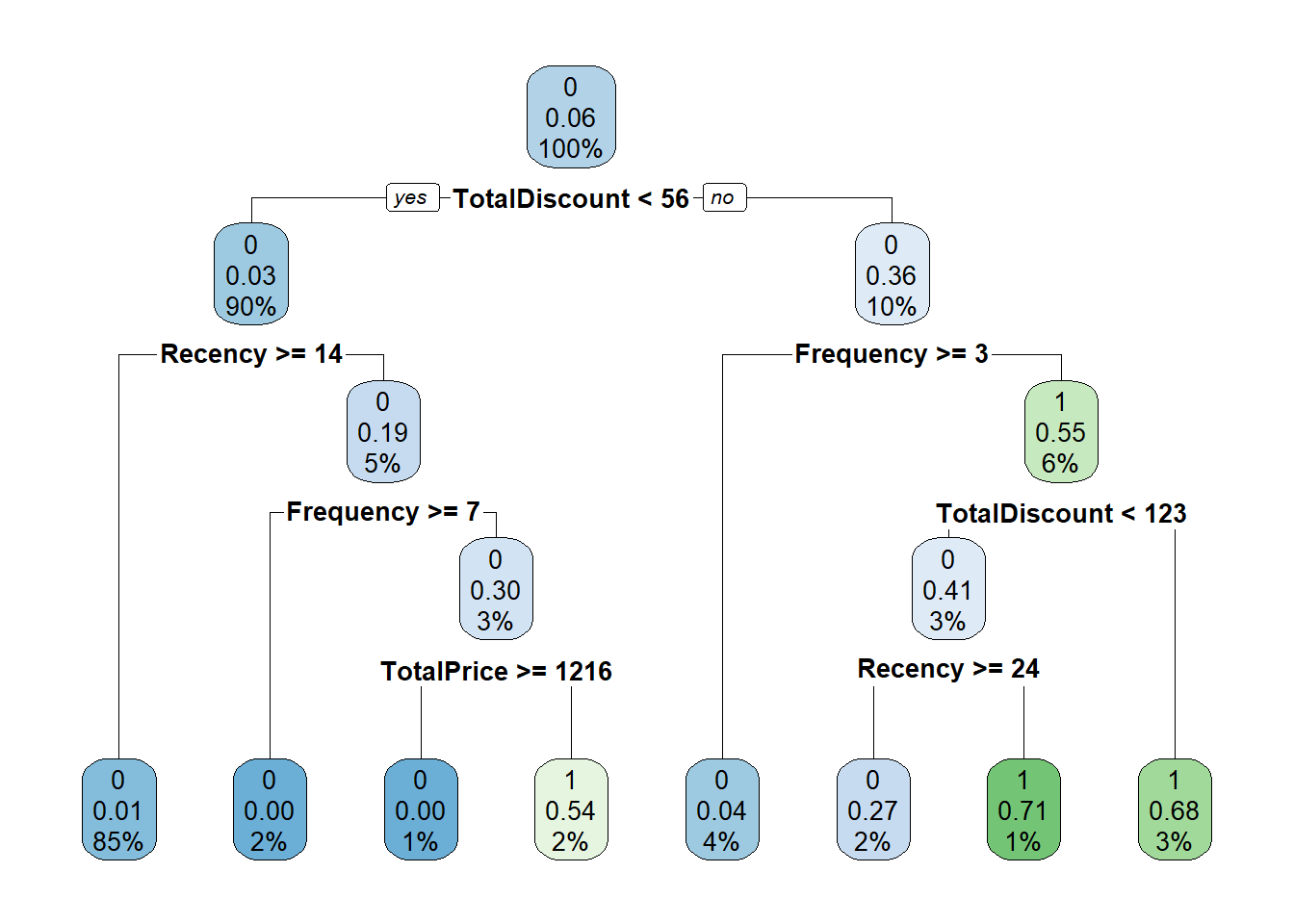
It is easy to observe that lower cost complexity parameter values lead to much more complex trees. But how should we determine the ideal cost complexity? Exactly! By checking the AUC performance of different values on the validation set! We are starting to see a pattern here.
candidates <- seq(1e-05, 0.2, by = 0.001)
aucstore <- numeric(length(candidates))

j <- 0
for (i in candidates) {
    j <- j + 1
    tree <- rpart(yTRAIN ~ ., control = rpart.control(cp = i),
        BasetableTRAIN)
    predTree <- predict(tree, BasetableVAL)[, 2]
    aucstore[j] <- AUC::auc(roc(predTree, yVAL))
    if (j%%20 == 0)
        cat(j/length(candidates) * 100, "% finished\n")
}
## 10 % finished
## 20 % finished
## 30 % finished
## 40 % finished
## 50 % finished
## 60 % finished
## 70 % finished
## 80 % finished
## 90 % finished
## 100 % finished# Let's determine the optimal cp value
plot(candidates, aucstore, type = "l")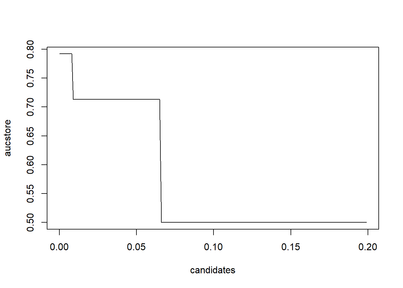
Optimal cp value seems to be far off from its default value of 0.01. This once again shows the importance of hyperparameter tuning.
# Optimal cp
candidates[which.max(aucstore)]
## [1] 1e-05# Now build a tree with the optimal cp
tree <- rpart(yTRAINbig ~ ., control = rpart.control(cp = candidates[which.max(aucstore)]),
BasetableTRAINbig)
predTREE <- predict(tree, BasetableTEST)[, 2]
# Evaluate performance
AUC::auc(roc(predTREE, yTEST))## [1] 0.8920165Let’s have final look at our optimal decision tree.
rpart.plot(tree)