4 Advanced Modeling
This chapter will cover the concepts seen in Advanced Modeling. We will discuss more in detail how to implement several advanced algorithms. Make sure that you go over the video and slides before going over this chapter.
4.1 Nonlinear models
In the previous chapter, we saw the most popular models in predictive analytics. While the linear regression and logistic regression models are very popular, they suffer from some downsides. The largest one, as we already discussed, being the assumption of linearity. Very few relationships are linear in real life situations. This was why a very simple decision tree model is often capable of outperforming logistic regression models.
However, decision trees are not the only solution to this issue of nonlinearity and also have some major downside (i.e., their instability). Let us start with regression models. The most straightforward extension to linear regression models are polynomial regression models as we already shortly covered during last week’s session. In polynomial regression models, we add polynomial terms to our regression model. The assumed relationship is then altered to a nonlinear variant. While this is already much more flexible, we still have a relationship which is strictened to its formulation.
Consider the example below. We have a dataset of football player attributes and their overall rating. When we inspect the relationship between goalkeeper reflexes and overall rating, we get a special non-monotonic relationship. This is because the left hand of the graph represents ‘field players’, for which GK reflexes are of no importance when estimating their overall rating. The right hand side, on the other hand, are actual goal keepers, for which GK reflexes of course is the most important determinant.
# Load the necessary packages Load the tidyverse package
if (!require("pacman")) install.packages("pacman")
require("pacman", character.only = TRUE, quietly = TRUE)

p_load(tidyverse)

# Read in the data
football <- read_csv("C:\\Users\\matbogae\\OneDrive - UGent\\PPA22\\PredictiveAnalytics\\Book_2022\\data codeBook_2022\\football_players.csv")
## Rows: 10390 Columns: 32## -- Column specification --------------------------
## Delimiter: ","
## chr (1): player_name
## dbl (31): overall_rating, potential, crossing,...##
## i Use `spec()` to retrieve the full column specification for this data.
## i Specify the column types or set `show_col_types = FALSE` to quiet this message.# Have a glimpse
football %>%
glimpse()## Rows: 10,390
## Columns: 32
## $ player_name <chr> "Aaron Appindangoye",~
## $ overall_rating <dbl> 63.60000, 66.96970, 6~
## $ potential <dbl> 67.60000, 74.48485, 7~
## $ crossing <dbl> 48.60000, 70.78788, 6~
## $ finishing <dbl> 43.60000, 49.45455, 5~
## $ heading_accuracy <dbl> 70.60000, 52.93939, 5~
## $ short_passing <dbl> 60.60000, 62.27273, 6~
## $ volleys <dbl> 43.60000, 29.15152, 5~
## $ dribbling <dbl> 50.60000, 61.09091, 6~
## $ curve <dbl> 44.60000, 61.87879, 6~
## $ free_kick_accuracy <dbl> 38.60000, 62.12121, 5~
## $ long_passing <dbl> 63.60000, 63.24242, 6~
## $ ball_control <dbl> 48.60000, 61.78788, 6~
## $ acceleration <dbl> 60.00000, 76.00000, 7~
## $ sprint_speed <dbl> 64.00000, 74.93939, 7~
## $ agility <dbl> 59.00000, 75.24242, 7~
## $ reactions <dbl> 46.60000, 67.84848, 5~
## $ balance <dbl> 65.00000, 84.72727, 8~
## $ shot_power <dbl> 54.60000, 65.90909, 6~
## $ jumping <dbl> 58.00000, 75.30303, 6~
## $ stamina <dbl> 54.00000, 72.87879, 7~
## $ strength <dbl> 76.00000, 51.75758, 7~
## $ long_shots <dbl> 34.60000, 54.12121, 5~
## $ aggression <dbl> 65.80000, 65.06061, 5~
## $ interceptions <dbl> 52.20000, 57.87879, 4~
## $ positioning <dbl> 44.60000, 51.48485, 6~
## $ vision <dbl> 53.60000, 57.45455, 6~
## $ penalties <dbl> 47.60000, 53.12121, 6~
## $ marking <dbl> 63.80000, 69.39394, 2~
## $ standing_tackle <dbl> 66.00000, 68.78788, 2~
## $ sliding_tackle <dbl> 67.80000, 71.51515, 2~
## $ gk_reflexes <dbl> 7.60000, 12.90909, 13~# Make a quick plot
plot(football$gk_reflexes, football$overall_rating)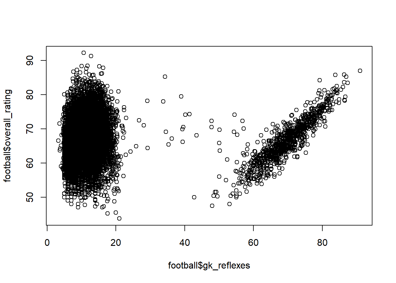
To solve this non-monotonicity, we could try to fit a (quadratic) polynomial on this relationship. A quick modeler would actually be very pleased with this result, as all terms are highly significant.
# Add a second degree polynomial
football <- football %>%
    mutate(reflex_squared = football$gk_reflexes^2)
polynomial <- lm(overall_rating ~ gk_reflexes + reflex_squared,
    football)

# Or shorter polynomial <- lm(overall_rating ~
# poly(gk_reflexes,2,raw = TRUE) , football) Set raw = TRUE
# to get the raw polynomials, otherwise the orthogonal ones
# are returned

summary(polynomial)
##
## Call:
## lm(formula = overall_rating ~ gk_reflexes + reflex_squared, data = football)
##
## Residuals:
## Min 1Q Median 3Q Max
## -22.3967 -3.9914 -0.0364 4.0465 25.3498
##
## Coefficients:
## Estimate Std. Error t value
## (Intercept) 67.9298334 0.2264452 299.984
## gk_reflexes -0.1203310 0.0217860 -5.523
## reflex_squared 0.0016866 0.0002673 6.310
## Pr(>|t|)
## (Intercept) < 2e-16 ***
## gk_reflexes 3.41e-08 ***
## reflex_squared 2.90e-10 ***
## ---
## Signif. codes:
## 0 '***' 0.001 '**' 0.01 '*' 0.05 '.' 0.1 ' ' 1
##
## Residual standard error: 6.142 on 10387 degrees of freedom
## Multiple R-squared: 0.0055, Adjusted R-squared: 0.005309
## F-statistic: 28.72 on 2 and 10387 DF, p-value: 3.634e-13However, when we plot this predicted relationship, we observe that it is not representative of the ‘true’ underlying relationship.
# Make a synthetic data set to get the fitted predicted
# relationship
synthetic <- data.frame(gk_reflexes = seq(0, 100), reflex_squared = seq(0,
    100)^2)
predictions <- predict(polynomial, synthetic)

# plot
plot(football$gk_reflexes, football$overall_rating)
lines(seq(0, 100), predictions, col = "red")
So, how should we handle such complex nonlinear relationships? The answer lays in smoothing splines. These automatically fit to the data and put little restraints on the assumed relationship . To fit these splines, we use the gam package’s function gam. Note that there is another GAM package called mgcv, which is a more efficient and more extensive implementation of GAM (e.g., there are more options for splines and even penalized splines can be used). Since we want to stay as close to the theory as possible, we choose the original gam implementation by the authors Hastie and Tibshirani, however, feel free to experiment with the mgcv package. By adding a s() function around your independent variable, the package knows it has to compute a regression spline of these variables. For variables where this s() is omitted, it will create regular regression coefficients.
# Load gam this is the package created by the creators
# Hastie and Tishirani Hence our choice for this pacakge
p_load(gam)
# Fit a GAM model with flexible regression splines
gam <- gam::gam(overall_rating ~ s(gk_reflexes), data = football)
predictions <- predict(gam, synthetic)
# Plot again
plot(football$gk_reflexes, football$overall_rating)
lines(seq(0, 100), predictions, col = "red")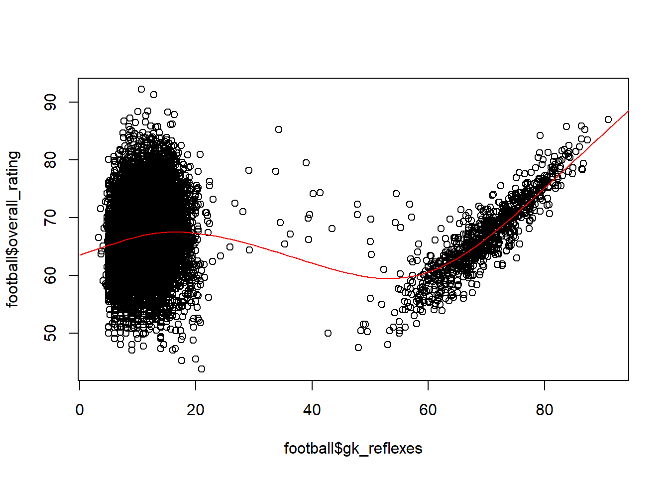
The regression spline already reflects much better the underlying relationship with little influence at low values and a high positive relationship at high values. This is also reflected in the AIC scores of the two models. The AIC is lower for the GAM (regression spline), which reflects a better goodness-of-fit. Note how such goodness-of-fit measures (AIC, R-squared, …) are especially useful when no test set is used, however they should never be used to replace a proper test design!
AIC(polynomial)## [1] 67210.01AIC(gam)## [1] 66327.78The beneficial effects of regression splines are put into the highly performant GAMs. These add (hence the name generalized additive models) the regression splines of various predictors into one model, resulting into a highly performant predictive model, with little fine tuning required. Let us compare the performance of a GAM model to a ‘default’ linear regression model.
# Before modeling a GAM, let's have a look at the data
football %>%
    glimpse()
## Rows: 10,390
## Columns: 33
## $ player_name <chr> "Aaron Appindangoye",~
## $ overall_rating <dbl> 63.60000, 66.96970, 6~
## $ potential <dbl> 67.60000, 74.48485, 7~
## $ crossing <dbl> 48.60000, 70.78788, 6~
## $ finishing <dbl> 43.60000, 49.45455, 5~
## $ heading_accuracy <dbl> 70.60000, 52.93939, 5~
## $ short_passing <dbl> 60.60000, 62.27273, 6~
## $ volleys <dbl> 43.60000, 29.15152, 5~
## $ dribbling <dbl> 50.60000, 61.09091, 6~
## $ curve <dbl> 44.60000, 61.87879, 6~
## $ free_kick_accuracy <dbl> 38.60000, 62.12121, 5~
## $ long_passing <dbl> 63.60000, 63.24242, 6~
## $ ball_control <dbl> 48.60000, 61.78788, 6~
## $ acceleration <dbl> 60.00000, 76.00000, 7~
## $ sprint_speed <dbl> 64.00000, 74.93939, 7~
## $ agility <dbl> 59.00000, 75.24242, 7~
## $ reactions <dbl> 46.60000, 67.84848, 5~
## $ balance <dbl> 65.00000, 84.72727, 8~
## $ shot_power <dbl> 54.60000, 65.90909, 6~
## $ jumping <dbl> 58.00000, 75.30303, 6~
## $ stamina <dbl> 54.00000, 72.87879, 7~
## $ strength <dbl> 76.00000, 51.75758, 7~
## $ long_shots <dbl> 34.60000, 54.12121, 5~
## $ aggression <dbl> 65.80000, 65.06061, 5~
## $ interceptions <dbl> 52.20000, 57.87879, 4~
## $ positioning <dbl> 44.60000, 51.48485, 6~
## $ vision <dbl> 53.60000, 57.45455, 6~
## $ penalties <dbl> 47.60000, 53.12121, 6~
## $ marking <dbl> 63.80000, 69.39394, 2~
## $ standing_tackle <dbl> 66.00000, 68.78788, 2~
## $ sliding_tackle <dbl> 67.80000, 71.51515, 2~
## $ gk_reflexes <dbl> 7.60000, 12.90909, 13~
## $ reflex_squared <dbl> 57.76000, 166.64463, ~# Let's decide to delete our quadratic term, the player
# name and football potential for our modeling exercise
football <- football %>%
dplyr::select(-c(reflex_squared, player_name, potential))set.seed(123)
# Evaluation function
RMSE <- function(true, predictions) {
return(sqrt(mean((true - predictions)^2)))
}
# Train/val/test splitting: 60/20/20 split
allind <- sample(x = 1:nrow(football), size = nrow(football))
trainind <- allind[1:round(length(allind) * 0.6)]
valind <- allind[(round(length(allind) * 0.6) + 1):round(length(allind) *
(0.8))]
testind <- allind[(round(length(allind) * (0.8)) + 1):length(allind)]
train <- football[trainind, ]
val <- football[valind, ]
test <- football[testind, ]
trainbig <- rbind(train, val)
# Model a GAM apply a flexible spline on each variable to
# see what happens
gam <- gam(overall_rating ~ s(gk_reflexes) + s(crossing) + s(finishing) +
s(heading_accuracy) + s(short_passing) + s(volleys) + s(dribbling) +
s(curve) + s(free_kick_accuracy) + s(long_passing) + s(ball_control) +
s(acceleration) + s(sprint_speed) + s(agility) + s(reactions) +
s(balance) + s(shot_power) + s(jumping) + s(stamina) + s(strength) +
s(long_shots) + s(aggression) + s(interceptions) + s(positioning) +
s(vision) + s(penalties) + s(marking) + s(standing_tackle) +
s(sliding_tackle), data = train)
# Compare with a linear model
lin_model <- lm(overall_rating ~ ., train)
# Make predictions
predictions_gam <- predict(gam, val)
predictions_lin <- predict(lin_model, val)
# Look at your performance
cat("GAM RMSE: ", RMSE(val$overall_rating, predictions_gam),
"\n")## GAM RMSE: 1.781093cat("LM RMSE: ", RMSE(val$overall_rating, predictions_lin), "\n")## LM RMSE: 2.981416# So the improvement is
abs((RMSE(val$overall_rating, predictions_gam) - RMSE(val$overall_rating,
predictions_lin))/RMSE(val$overall_rating, predictions_lin))## [1] 0.4026015Our nonlinear GAM model was able to reduce the error of our model by over 40% on the validation set! This is ofcourse a marvelous improvement, so why are not all statisticians switching to using GAMs instead of linear regression models? Well, linear regression coefficient interpretation remains extremely easy to interpret. But one should be cautious, as a linear model has a lot of assumptions and any violations of these assumptions makes the coefficients and the point estimates highly unreliable! When you are predicting point estimates (as we are doing with the exact rating of players), you are advised to always consider a GAM model in your list of evaluated models.
# Build the final model
gam_final <- gam(overall_rating ~ s(gk_reflexes) + s(crossing) +
    s(finishing) + s(heading_accuracy) + s(short_passing) + s(volleys) +
    s(dribbling) + s(curve) + s(free_kick_accuracy) + s(long_passing) +
    s(ball_control) + s(acceleration) + s(sprint_speed) + s(agility) +
    s(reactions) + s(balance) + s(shot_power) + s(jumping) +
    s(stamina) + s(strength) + s(long_shots) + s(aggression) +
    s(interceptions) + s(positioning) + s(vision) + s(penalties) +
    s(marking) + s(standing_tackle) + s(sliding_tackle), data = trainbig)

# Predict and evaluate
final_predictions <- predict(gam_final, test)
cat("Final GAM performance: ", RMSE(test$overall_rating, final_predictions))
## Final GAM performance: 1.653585The estimated RMSE on the test set is similar (even smaller) to the one we had on the validation set, which is good. The better performance of the model compared to the linear regression model can be explained when plotting the fitted splines.
plot(gam_final, terms = "s(gk_reflexes)")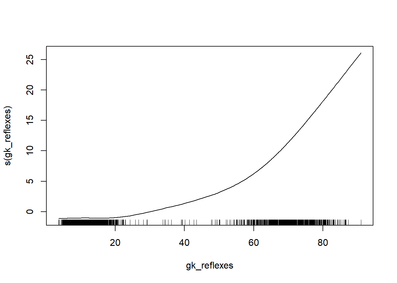
4.2 Naïve Bayes
Naïve Bayes is a classifier which uses the Bayes theorem (posterior = (likelihood * prior) / normalizing constant) to calculate the posterior for various independent variables. This is done indepently for all classifiers, which means that the posterior \(P(Y|X_1)\) does not account for the posterior \(P(Y|X_2)\). This implies that the algorithm assumes that there is no relationship between the various predictors. As this is often not the case, the algorithm is called naive Bayes.
To understand the reasoning behind the algorithm, we will deploy a small example on a self-fabricated dataset. On this dataset we will try to build a naive Bayes model ourselves, which we use to predict the churn of a new instance: \(P(churn=1|X_{tenure}=long \& X_{spend}=high)\).
In Bayes theorem, we know that this is the same as dividing:
\[\begin{equation} P( X_{tenure}=long | churn = 1 ) P( X_{spend}=high | churn = 1 ) P( churn = 1) \end{equation}\]
by:
\[\begin{equation} P(X_{tenure}=long \& X_{spend}=high) = \\ P(X_{tenure}=long | churn = 0 ) P( X_{spend}=high | churn = 0 ) P( churn = 0) \\ + P( X_{tenure}=long | churn = 1 ) P( X_{spend}=high | churn = 1 ) P( churn = 1) \end{equation}\]
# Create small data set
df <- data.frame(churn = c(1, 0, 1, 1, 1, 0, 1, 0, 1, 1, 1, 1,
    1, 0), tenure = c("medium", "long", "short", "medium", "medium",
    "medium", "short", "long", "long", "medium", "long", "short",
    "short", "medium"), spend = c("high", "high", "high", "medium",
    "low", "low", "low", "medium", "low", "medium", "medium",
    "medium", "high", "medium"))
A first term we need to calculate is the prior: the probability of 1.
# Distribution P(Y)
(py <- table(df$churn)/sum(table(df$churn)))
##
## 0 1
## 0.2857143 0.7142857# We need P(Y=1)
(prior <- py[2])## 1
## 0.7142857After we have calculated the prior, we need to calculate the likelihood \(P(X=k|Y=1)\). As we have two independent variables, we will calculate two cross-tabulations.
# Likelihood distribution tenure
(ll_tenure <- t(t(table(df$tenure, df$churn))/colSums(table(df$tenure,
    df$churn))))
##
## 0 1
## long 0.5 0.2
## medium 0.5 0.4
## short 0.0 0.4# Likelihood distribution spend
(ll_spend <- t(t(table(df$spend, df$churn))/colSums(table(df$spend,
df$churn))))##
## 0 1
## high 0.25 0.30
## low 0.25 0.30
## medium 0.50 0.40Remember: we wanted to predict \(P(churn=1|X_{tenure}=long \& X_{spend}=high)\). This means we need the respective parts from the ll_tenure (P(long|1)) and ll_spend (P(high|1)) distributions.
(likelihood_long <- ll_tenure[1, 2])## [1] 0.2(likelihood_high <- ll_spend[1, 2])## [1] 0.3Hereby, we can already easily calculate our numerator (P( Xtenure=long | churn = 1 ) x P( Xspend=high | churn = 1 ) x P( churn = 1)):
(numerator <- likelihood_long * likelihood_high * prior)## 1
## 0.04285714We now still need to do our denominator (normalizing constant): \[\begin{equation} P(X_{tenure}=long \& X_{spend}=high) = \\ P(X_{tenure}=long | churn = 0 ) P( X_{spend}=high | churn = 0 ) P( churn = 0) \\ + P( X_{tenure}=long | churn = 1 ) P( X_{spend}=high | churn = 1 ) P( churn = 1) \end{equation}\]
(normalizing <- ll_tenure[1, 1] * ll_spend[1, 1] * py[1] + ll_tenure[1,
    2] * ll_spend[1, 2] * py[2])
## 0
## 0.07857143# note that second term is equal to
# likelihood_long*likelihood_high*prior or the numeratorThe final prediction then leads to:
(pred <- numerator/normalizing)## 1
## 0.5454545We will see if this prediction follows the same behavior as the predictions made by the naive Bayes algorithm as implemented by the e1071 package. And indeed the first input (long & high) gives the some probability estimate as our self-defined method. As a home exercise, try to also make the prediction for the second observation (short & medium).
p_load(e1071)

# fit model
NB <- naiveBayes(x = df[, 2:3], y = df[, 1])

# create new unseen data. Make sure that all variables have
# the same factor levels as in the fitted model!
new <- data.frame(tenure = factor(c("long", "short"), levels = c("long",
    "medium", "short")), spend = factor(c("high", "medium"),
    levels = c("high", "low", "medium")))
(predNB <- predict(NB, new, type = "raw", threshold = 0.001)[,
    2])
## [1] 0.5454545 0.9987516This is relatively straightforward, but when dealing with continuous variables, the computation becomes more complex as it uses gaussian probability density functions (another option can be to bin the continuous variables and then just use the formula as it is). So just use provided package to deploy a naive Bayes model.
We will now deploy the naive Bayes algorithm on a more realistic situation. Let us assume we want to predict whether a football player is a top performer or not. To do so, we discretize the overall_rating value in our football dataset.
set.seed(123)

# Create the dependent variable
football <- football %>%
    mutate(top_player = as.factor(ifelse(overall_rating > 75,
        1, 0))) %>%
    dplyr::select(-overall_rating)

# Split
allind <- sample(x = 1:nrow(football), size = nrow(football))
trainind <- allind[1:round(length(allind) * 0.6)]
valind <- allind[(round(length(allind) * 0.6) + 1):round(length(allind) *
    (0.8))]
testind <- allind[(round(length(allind) * (0.8)) + 1):length(allind)]
train <- football[trainind, ]
val <- football[valind, ]
test <- football[testind, ]
trainbig <- rbind(train, val)

# Isolate the dependent variable
y_train <- train$top_player
y_val <- val$top_player
y_test <- test$top_player
y_trainbig <- trainbig$top_player

train$top_player <- val$top_player <- test$top_player <- trainbig$top_player <- NULL

# First model attempt
library(AUC)
NB <- naiveBayes(y_train ~ ., train)
predNB <- predict(NB, val, type = "raw", threshold = 0.001)[,
    2]
AUC::auc(roc(predNB, factor(y_val)))
## [1] 0.8576572As the task is fairly simple (remember the nicely fitted spline of the GAM), we get a relatively high AUC. However, if you want to achieve an even higher accuracy, you should think out-of-the-box. Remember from the theory that naive Bayes assumes independence of predictors. However, it is highly likely that in this situation this assumption is violated as some features clearly could be categorized in some larger groups (defensive skills, attacking skills, physical performance, etc.). Hence, you should make sure that the features are independent.
Now think back about your Social Media and Web Analytics course, where you saw Singular Value Decomposition (SVD), as a technique that will allow you to reduce the number of predictors as well as the collinearity across predictors. (https://blogs.oracle.com/r/using-svd-for-dimensionality-reduction for those that want a quick refresher or just have a look at the slides of SMWA).
# Let's perform SCV on the predictors of the training set
svd <- svd(train)

# Remember d represents the concept matrix u represents the
# term (player) by concept matrix v represents the concept
# by predictor matrix
svd %>%
    glimpse()
## List of 3
## $ d: num [1:29] 24217 3426 2250 1454 1248 ...
## $ u: num [1:6234, 1:29] -0.0141 -0.0129 -0.0122 -0.0141 -0.0138 ...
## $ v: num [1:29, 1:29] -0.178 -0.16 -0.186 -0.201 -0.159 ...# Make a scree plot to determine the number of concepts to
# retain
plot(seq(1, 29), svd$d, "l") #just use 5 dimensions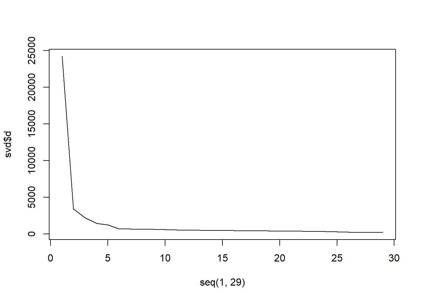
# reduce columns: we always use the model fitted on the
# training set to reform the columns so use matrix
# computation
train_reduced <- as.matrix(train) %*% svd$v[, 1:5, drop = FALSE] %*%
    diag((svd$d)[1:5, drop = FALSE])
val_reduced <- as.matrix(val) %*% svd$v[, 1:5, drop = FALSE] %*%
    diag((svd$d)[1:5, drop = FALSE])
# Rebuild naive Baeys with the concepts
NB_svd <- naiveBayes(y_train ~ ., data = data.frame(train_reduced))
predNB2 <- predict(NB_svd, data.frame(val_reduced), type = "raw",
threshold = 0.001)[, 2]
AUC::auc(roc(predNB2, factor(y_val)))## [1] 0.8741453As expected, the AUC improved (just imagine the problem of assumed independence when dealing with hundreds of predictors). Also, take a short moment to reflect on the differences in model interpretability (how do we interpret svd dimensions?).
Remember to always compare different methods on the val set, before moving on to the final evaluation on the test set.
# Reduce trainbig and test Note that you could also rebuild
# the SVD on the trainbig Since train is a subset there is
# no change of data leakage, so you can just use the
# original SVD However, a purist might argue that you
# should rebuild ...
trainbig_reduced <- as.matrix(trainbig) %*% svd$v[, 1:5, drop = FALSE] %*%
    diag((svd$d)[1:5, drop = FALSE])
test_reduced <- as.matrix(test) %*% svd$v[, 1:5, drop = FALSE] %*%
    diag((svd$d)[1:5, drop = FALSE])

NB3 <- naiveBayes(y_trainbig ~ ., data = data.frame(trainbig_reduced))
predNB3 <- predict(NB3, data.frame(test_reduced), type = "raw",
    threshold = 0.001)[, 2]
print(AUC::auc(roc(predNB3, factor(y_test))))
## [1] 0.8802066Note that dependent on the split, your test performance can be lower than your val performance and SVD might have a worse performance than the normal NB. Therefore, it is important using cross-validation (for model selection) on a limited data set, we will have more stable estimates of each model, which are then also finally evaluated on a never seen test set.
4.3 K nearest neighbors
KNN has to be one of the most simple predictive algorithms in the data scientist’s toolbox. It uses the very simple reasoning: ‘When there is an unseen observation, which K elements are most similar (nearest) to this observation and what is their average (most common) value?’
This description already identifies the two most important parameters of the algorithm: the number of neighbours that you take into consideration (K) and the way you define these neighbors: the similarity measure. The most popular similarity measure is Euclidean distance, but as you will see during the session on unsupervised learning (cf. infra), many others exist and in some situations, it might also be useful to deploy these.
We will now create our own KNN classifier. Our methodology requires all features to be numeric, so ensure that this is the case before you try to deploy this method! (Just think about how someone should compute the Euclidean distance between two categories. It is exactly this kind of difficulties which causes other similarity measures to be used in certain situations)
As a first step, you should always standardize the variables. This is even more important in KNN than in other algorithms. Just think of following example: you have three people of which you have both the annual income and their average score (on 10) as students: P1(22000, 9.1), P2(23000,8.8), P3(21500,5.7). While such little information of course is too scarce to truly distinguish people, one would intuitively think of P1 and P2 of being more similar than P3. When deploying KNN on unscaled data, however, one would identify P1 and P3 as most similar, because the difference in income difference (500 vs 1000) is much larger than the difference in grade (3.4 vs 0.3).
To scale the data remember that we once again only use information from the respective training sets to avoid data leakage.
# Let's standardize our variables Note that here we will be
# using a more vectorized/mathematical approach to
# standardization Remember from the preprocessing chapter
# that you can also use the tidyverse approach It is
# totally up to you with which coding paradigm you feel
# most comfortable

# scaling for sets used during parameter tuning
stdev <- sapply(train, sd)
means <- sapply(train, mean)
trainKNN <- data.frame(t((t(train) - means)/stdev))
valKNN <- data.frame(t((t(val) - means)/stdev))

# scaling for hold-out performance estimation
stdev <- sapply(trainbig, sd)
means <- sapply(trainbig, mean)
trainKNNbig <- data.frame(t((t(trainbig) - means)/stdev))
testKNN <- data.frame(t((t(test) - means)/stdev))
We decide upon using the Euclidean distance as similarity measure. To do so, we use the FNN package’s knnx.index function, which finds the k nearest neighbors of an instance. Multiple search algorithms are possible and can be provided with the algorithm argument. The default brute search equals a complete search of all possible neighbours. Note how query signifies the data we want to find the neighbors of and data the population we are using to search for neighbors. As we already determined the similarity measure (Euclidean distance), we only have to determine the optimal number of neighbors K.
p_load(FNN)

set.seed(123)

auc <- numeric()
for (k in 1:40) {
  #retrieve the indicators of the k nearest neighbors of the query data
  indicatorsKNN <- as.integer(knnx.index(data=trainKNN, query=valKNN, k=k))
  #retrieve the actual y from the training set
  predKNN <- as.integer(as.character(y_train[indicatorsKNN]))
  #if k > 1 then we take the proportion of 1s
  predKNN <- rowMeans(data.frame(matrix(data=predKNN, ncol=k, nrow=nrow(valKNN))))
  #Compute AUC
  auc[k] <- AUC::auc(roc(predKNN,factor(y_val)))
}

plot(1:40,auc,type="l", xlab="k")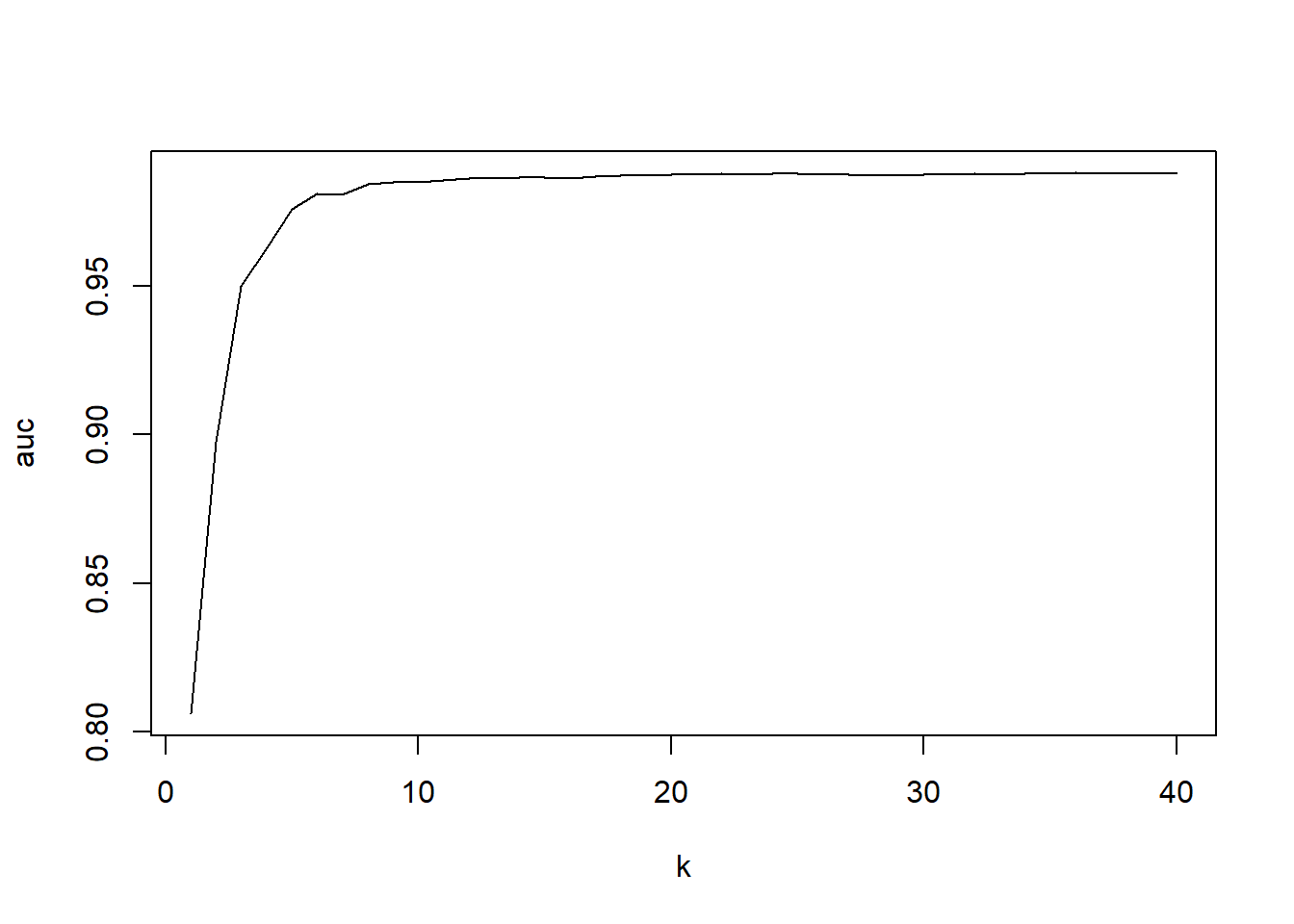
We clearly see a steep rise in the beginning of the curve. Too few neighbors would lead to a too high influence of some data points. However, above K around 30, we see a stagnation of the curve. If you would include even more neighbors the model starts to learn too many data points which are not real ‘neighbors’ and performance would again decline.
(k <- which.max(auc))## [1] 36# retrieve the indicators of the k nearest neighbors of the
# query data
indicatorsKNN <- as.integer(knnx.index(data = trainKNNbig, query = testKNN,
k = k))
# retrieve the actual y from the training set
predKNNoptimal <- as.integer(as.character(y_trainbig[indicatorsKNN]))
# if k > 1 then we take the proportion of 1s
predKNNoptimal <- rowMeans(data.frame(matrix(data = predKNNoptimal,
ncol = k, nrow = nrow(testKNN))))
# Evaluate
AUC::auc(roc(predKNNoptimal, factor(y_test)))## [1] 0.9886304plot(roc(predKNNoptimal, factor(y_test)))
The classifier’s performance is quite impressive. It heavily outperforms other classifiers we tried up until now. This is partially due to the nature of our problem, as KNN models are often not among top performing models. The fact that the model performs so well here however signifies that each prediction problem is unique and that you, as a data scientist, should always consider multiple methods.
4.4 Support vector machines
The Support Vector Machine (SVM) technique creates an optimal hyperplane that distinguishes between categories, also known as the maximal margin hyperplane. The maximal margin hyperplane is the hyperplane that separates two classes with maximal margin (maximal distance to data points). Two steps are important in ensuring that this classifier delivers satisfying performance. Firstly, we need to consider that two categories are often not perfectly separable in real life. This means we have to account for a non-exact maximal margin hyperplane (as this could not be constructed when two classes are not perfectly separable). This is where the cost parameter comes into play. It controls for the number of misclassifications (i.e., instances on the wrong side of the hyperplane) and determines the overall distance that all misclassifications can have to the hyperplane.
Another important consideration is the fact that a maximum margin classifier assumes a linear relationship between feature space and response, which is often unrealistic and leads to high bias. To allow for nonlinearities, the kernel trick is applied to the features space. A kernel function will make sure that non-linear boundaries are transformed to linear boundaries.To do so, the kernel function transforms 2 observations to enlarge the feature space.
This means that both the cost parameter and kernel function are important parameters to set. To further complicate things, each kernel function has its own important parameters, which differ across kernel functions. This results in a slightly more complicated hyperparameter tuning.
To understand the importance of the kernel trick: consider below example. We have a small data set which we want to use to build a classifier one by drawing a line (our maximal margin ‘hyperplane’).
x <- runif(100, min = -5, max = 5)
y <- factor(ifelse(x < 2 & x > -2, 1, 0))

plot(x, rep(1, length(x)), col = y)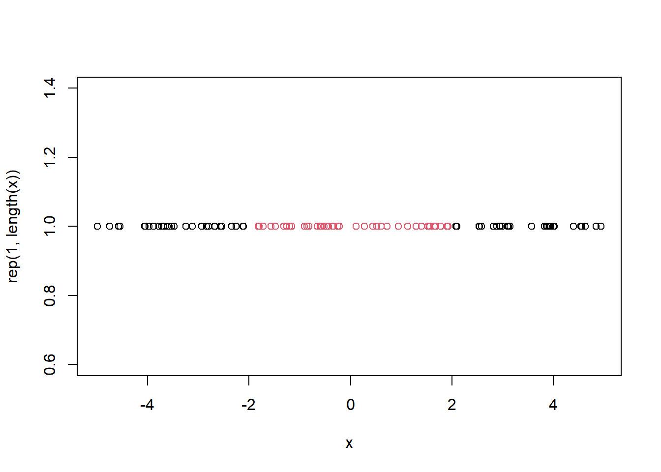
This could easily be done by two lines, but how do we do this with one line? By manipulating the feature space!
plot(x, x^2, col = y)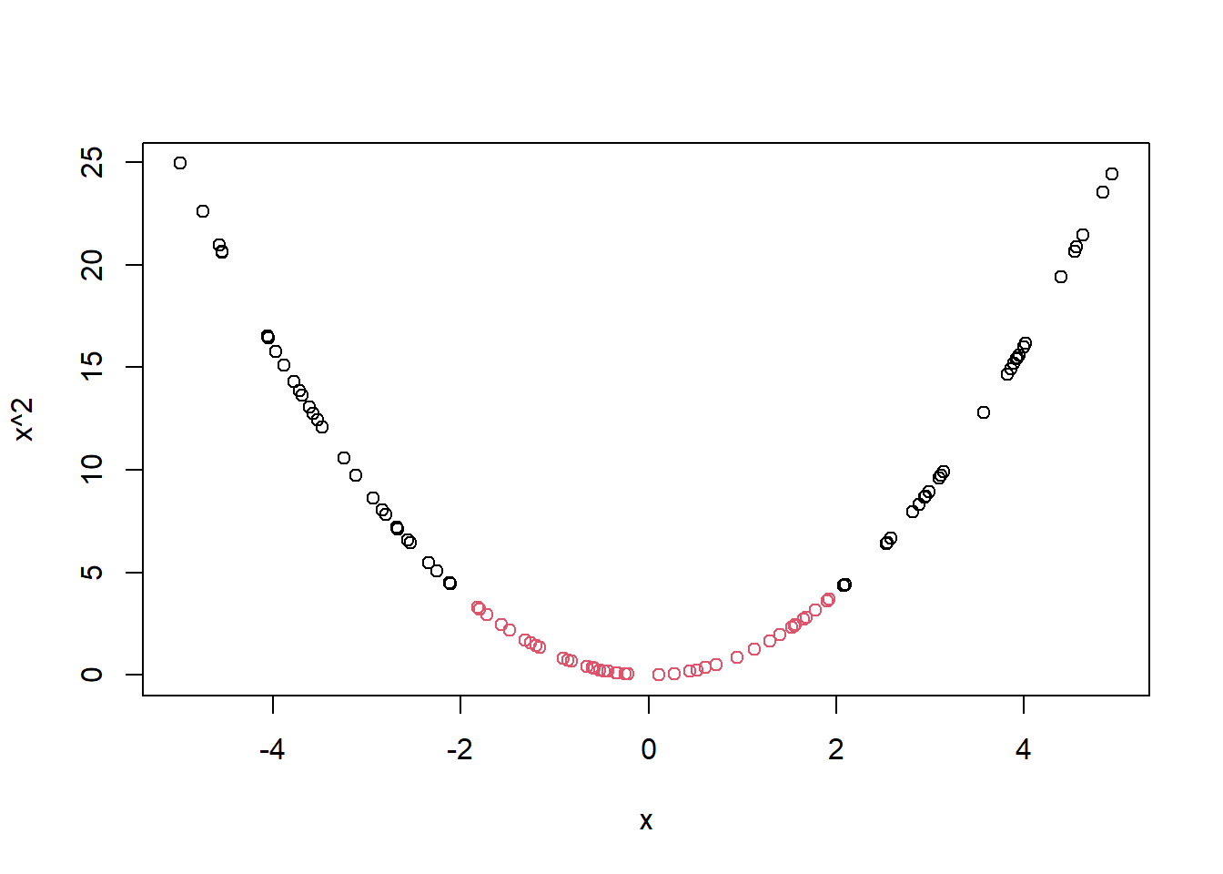
So why do we use kernels rather than simple feature manipulations? Because these manipulations have the potential to completely derail the dimensionality of the feature space. Consider following example.
case1 <- data.frame(c1=1:4,c2=c(1,2,1,2),c3=c(1,2,1,1))
rownames(case1) <- c('r1','r2','r3','r4')
head(case1)
## c1 c2 c3
## r1 1 1 1
## r2 2 2 2
## r3 3 1 1
## r4 4 2 1If we manipulate the feature space quadratically, we get 6 dimensions. Just imagine how large this could grow if we have many input features. If we would have 150 variables, we would get 11,325 columns!
case2 <- data.frame(c_1_square = case1$c1^2, c_2_square = case1$c2^2,
    c_3_square = case1$c3^2, c1_c2 = sqrt(2) * case1$c1 * case1$c2,
    c1_c3 = sqrt(2) * case1$c1 * case1$c3, c2_c3 = sqrt(2) *
        case1$c2 * case1$c3)
rownames(case2) <- c("r1", "r2", "r3", "r4")
head(case2)
## c_1_square c_2_square c_3_square c1_c2
## r1 1 1 1 1.414214
## r2 4 4 4 5.656854
## r3 9 1 1 4.242641
## r4 16 4 1 11.313708
## c1_c3 c2_c3
## r1 1.414214 1.414214
## r2 5.656854 5.656854
## r3 4.242641 1.414214
## r4 5.656854 2.828427A typical solution to this dimensionality problem would be to multiply the new matrix with its transpose:
(as.matrix(case2) %*% as.matrix(t(case2)))## r1 r2 r3 r4
## r1 9 36 25 49
## r2 36 144 100 196
## r3 25 100 121 225
## r4 49 196 225 441Which is exactly the same as deploying the kernel trick! The kernel trick is just much faster, resulting in both a performant (predictive) model as well as a fast model.
(as.matrix(case1) %*% as.matrix(t(case1)))^2## r1 r2 r3 r4
## r1 9 36 25 49
## r2 36 144 100 196
## r3 25 100 121 225
## r4 49 196 225 441Now that we understand the reasoning behind the SVM algorithm, let us try to deploy it on our NPC churn example. Since SVMs also based on the notion of distance it is important to standardize the data. A SVM will benefit most from standardization (question: why???). Luckily for us the svm function of e1071 scales the data by default. However, always check if this is done since this can give faulty results otherwise.
# Load the datasets
load("C:\\Users\\matbogae\\OneDrive - UGent\\PPA22\\PredictiveAnalytics\\Book_2022\\data codeBook_2022\\TrainValTest.Rdata")

# Load the package
p_load(e1071)


# tuning grid with the tuneMember function
SV.cost <- 2^(-5:-4)  #This is good range but takes a long time: 2^(-5:13)
SV.gamma <- 2^(-15:-14)  #This is good range but takes a long time: 2^(-15:3)
# For the polynomial kernel function gamma denotes scale
# (not very important).  For the radial basis kernel gamma
# denotes the inverse kernel width (very important).
SV.degree <- c(1, 2, 3)
SV.kernel <- c("radial", "polynomial")
result <- list()


# Make a convenience function to help you with the tuning
tuneMember <- function(call, tuning, xtest, ytest, predicttype = NULL,
    probability = TRUE) {
    if (require(AUC) == FALSE)
        install.packages("AUC")
    library(AUC)

    grid <- expand.grid(tuning)

    perf <- numeric()
    for (i in 1:nrow(grid)) {
        Call <- c(as.list(call), grid[i, ])
        model <- eval(as.call(Call))

        predictions <- predict(model, xtest, type = predicttype,
            probability = probability)

        if (class(model)[2] == "svm")
            predictions <- attr(predictions, "probabilities")[,
                "1"]

        if (is.matrix(predictions))
            if (ncol(predictions) == 2)
                predictions <- predictions[, 2]
        perf[i] <- AUC::auc(roc(predictions, ytest))
    }
    perf <- data.frame(grid, auc = perf)
    perf[which.max(perf$auc), ]
}

for (i in SV.kernel) {

    call <- call("svm", formula = as.factor(yTRAIN) ~ ., data = BasetableTRAIN,
        type = "C-classification", probability = TRUE)

    # the probability model for classification fits a
    # logistic distribution using maximum likelihood to the
    # decision values of the binary classifier

    if (i == "radial")
        tuning <- list(gamma = SV.gamma, cost = SV.cost, kernel = "radial")
    if (i == "polynomial")
        tuning <- list(gamma = SV.gamma, cost = SV.cost, degree = SV.degree,
            kernel = "polynomial")
    # tune svm
    result[[i]] <- tuneMember(call = call, tuning = tuning, xtest = BasetableVAL,
        ytest = as.factor(yVAL), probability = TRUE)
}

result
## $radial
## gamma cost kernel auc
## 2 6.103516e-05 0.03125 radial 0.5796544
##
## $polynomial
## gamma cost degree kernel
## 2 6.103516e-05 0.03125 1 polynomial
## auc
## 2 0.8308327Our tuneMember function returns the optimal settings per kernel and we see that the polynomial kernel outperforms the radial base kernel by far.
This time, this went relatively fluent. This is, however, not always the case. A common error message you may encounter is “reaching max number of iterations”. In short, that means the LIBSVM thinks it failed to find the maximum margin hyperplane, which may or may not be true. There are many reasons why this may happen, Things you could try:
-Make sure your classes are more or less balanced (have similar size).
-Try different C and ‘gamma’. Polynomial kernel in LIBSVM also has parameter coef0,as the kernel is (\(\gamma \cdot u'\cdot v + coef0)^{d}\).
# select the best set of parameters
auc <- numeric()
for (i in 1:length(result)) auc[i] <- result[[i]]$auc
result <- result[[which.max(auc)]]

# now predict using these optimal parameters
SV <- svm(as.factor(yTRAINbig) ~ ., data = BasetableTRAINbig,
    type = "C-classification", kernel = as.character(result$kernel),
    degree = if (is.null(result$degree)) 3 else result$degree,
    cost = result$cost, gamma = if (is.null(result$gamma)) 1/ncol(BasetableTRAINbig) else result$gamma,
    probability = TRUE)

# Compute the predictions for the test set
predSV <- as.numeric(attr(predict(SV, BasetableTEST, probability = TRUE),
    "probabilities")[, "1"])
head(predSV)
## [1] 0.05415212 0.05399342 0.05406043 0.05488607
## [5] 0.05394722 0.05392016AUC::auc(roc(predSV, yTEST))## [1] 0.7653111