Chapter 9 Data from web sources
In this chapter:
- Importing data from web repositories
9.1 Introduction
There is a lot of valuable data out there on the internet, just waiting for curious data analysts to find nuggets of insight in it. There are a variety of ways to access that data; in some cases, you can download a CSV or Excel file and then read that into R.
But the brilliant people that make up the R community have made our life a whole lot easier by creating packages that allow us to write R scripts that link directly to data we want. This is particularly valuable if you are accessing a data set that gets updated regularly (say, a weekly financial report or the results of a monthly survey).
The foundation of this connection to data sources on the internet are APIs (for Application Programming Interface). APIs allow two pieces of software to communicate. In the context of data access, a site will be set up with an API that defines how data can be accessed and how it will be provided.
In general, an API package will require a connection to the internet. In some cases, an API may require a user key be requested (a strategy the site may use to authenticate users or limit the number or size of requests).
There are two sorts of R packages that utilize APIs. The first are those that are dedicated to a particular source of data, such as a statistics agency. In addition to getting the data, these packages often have additional functions which do a lot of the initial manipulation of the data for us, getting it into a format that is useful for R.
The second type are beyond the scope of this book, and are those that allow us to connect to the raw data source. Often with these sources, we will need to do some wrangling of the data before we can use it. If you are interested in learning more about creating your own connections in R to websites that provide an API, the R package {httr2}(Wickham 2023) might be a good place to start.
9.2 R packages for direct connection
In this section, we will explore examples that allows access to the data repositories hosted by the UK Office of National Statistics and Statistics Canada. There are many other tools available; some are listed at the end of this chapter. Neither of these sites requires (at least at the time of writing) an API key.
9.2.1 Office of National Statistics (UK)
Our first example will be {onsr}, which downloads data directly from the UK’s Office of National Statistics (Vasilopoulos 2022).
For this, we would like to obtain time series data of retail sales.
The first thing we might want to do is explore what’s available in our area of interest. The ons_datasets() function gives a full list of the data that is currently available.
From this we will select “Retail sales data for Great Britain in value and volume terms, seasonally and non-seasonally adjusted”, which has the id value of “retail-sales-index”.
The function ons_ids() provides a list of the id column that is obtained from the ons_datasets function.
Another option is the ons_browse_qmi() function, which opens the relevant ONS page in your web browser software.
Finally, we will use the relevant id value in an ons_get() function to retrieve the data.
There are 42,400 rows in this data (as of 2023-06-14), with multiple variables for each month. Your analysis will require further filtering and selecting, but with the {onsr} package providing the access to the data, you are well on your way.
9.2.2 Statistics Canada
Statistics Canada, a department of the Government of Canada, provides a socioeconomic time series database known as “CANSIM”. The data posted to the database is most of the aggregate data collected by Statistics Canada on a regular basis, such as the Labour Force Survey (from which we get updates on the unemployment rate), the Consumer Price Index Survey (about inflation), and health-related information from pregnancy and births to life expectancy and deaths.
The package {cansim} (von Bergmann and Shkolnik 2021) uses the API that Statistics Canada has created in order to facilitate direct download of hundreds of data tables and thousands of individual time series.
One of the many tables related to international travel that is published in CANSIM is “Table: 24-10-0050-01 Non-resident visitors entering Canada, by country of residence”. 16
Here’s a screenshot of the table, showing the number of people arriving by their continent of residence.
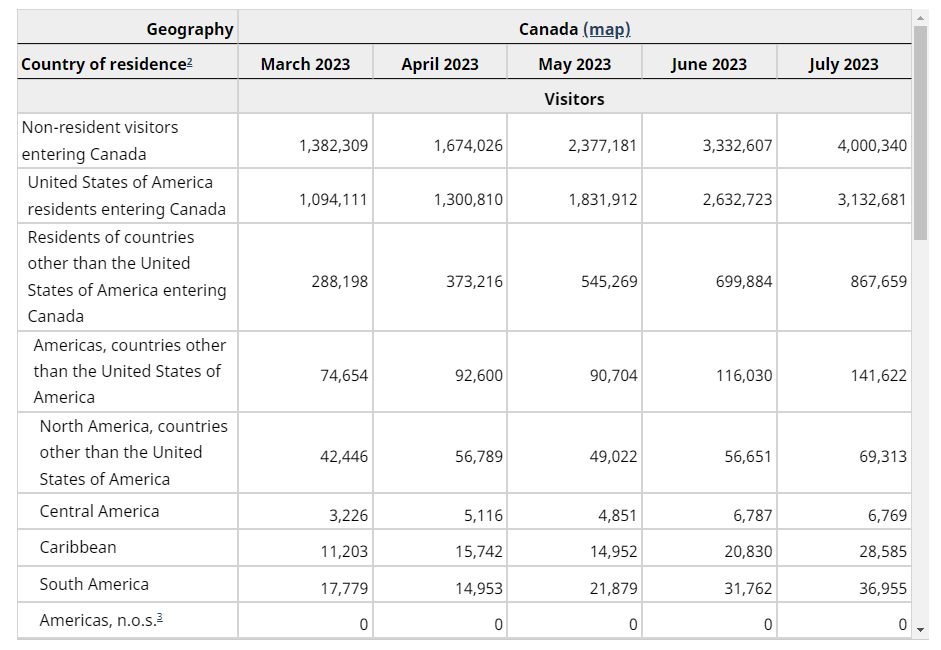
This table might be useful if you were developing a marketing campaign and you wanted to understand where tourists are coming from—the biggest markets and the fastest growing. But as shown, it is at too high a level; this is Canada by continent. For our purposes, we need to see specific country, those entering Canada via British Columbia, and a longer time series.
We could use the filters and fiddle around making sure we got the right selections and then download the data, but if we have to do that next month it is going to be inefficient. We could also first click on the “download options” button and select “download entire table…” but again, this is not the most efficient way to do this, since there are a few manual steps we have to take and then open the file into R and filter to select the series we want.
This is where the {cansim} package comes in.
Step 1: download the data.
- the
get_cansim()function takes the table number as the parameter, and connects to CANSIM and downloads the data into an R dataframe.
We will come back to filtering and variable selection along with working with date fields later, but here’s the code in R using the functions of the {dplyr} package to filter for the British Columbia cases during the month of June 2019:
travellers_bc <-
travellers |>
  filter(GEO == "British Columbia",
         REF_DATE == "2019-06")

glimpse(travellers_bc, width = 65)
There are 287 rows, one for each of the categories in the Country of residence variable. It’s important to note that these are not just countries, but the variable also includes subtotals. What if we just want a monthly report on a single continent? One option would be for us to filter the “COUNTRY” variable; here we filter for visitors from Europe.
One of the features of CANSIM and other similar tables is that the individual series are given a single identifier. In the case of CANSIM, these are called the “vector numbers”. Scroll to the right on this table, and you’ll see a variable called VECTOR. The vector identifier (sometimes called “the vector number” even though it’s a character string!) for European travellers entering Canada via British Columbia is v1277198032.
The {cansim} package also gives us a function to select a single vector number, so we can be more efficient still. We can speed up the download time and skip the filtering steps to get to the one we want. (Note that this function requires us to enter a start date, and converts the reference date variable to the YYYY-MM-DD format.)
This table has the shortcoming of not including the “GEO” or “Country of residence” variables, so we need to ensure that we have adequately documented what has been accessed.
The {cansim} package includes other very useful functions if you find yourself exploring Statistics Canada data sets.
The function get_cansim_table_overview() provides an abstract about the data table.
9.3 Other R packages for direct access to data
The following is an incomplete list (in alphabetical order by name) of other packages that have been developed to provide direct access to a specific web resource.
{bcdata} (Teucher et al. 2023) has tools to search, query, and download tabular and ‘geospatial’ data from the British Columbia Data Catalogue.
{fredr} (Boysel and Vaughan 2023) connects to the “Federal Reserve Economic Data”, or FRED, hosted by the Federal Reserve Bank of St. Louis. This data repository has (according to Wikipedia) over 800,000 economic time series from various sources.
{opendatatoronto} (Gelfand and City of Toronto 2022) provides a direct connection to the City of Toronto Open Data Portal.
The {readabs} (Cowgill et al. 2023) package downloads and tidies data from the Australian Bureau of Statistics.
{RBNZ} (Watson 2020) downloads data from the Reserve Bank of New Zealand Website.
{tidycensus} (Walker, Herman, and Eberwein 2023) has tools that connect to the United States Census Bureau and returns tidyverse-ready dataframes with the option of adding geographic details to allow for mapping. (See also (Walker 2023).)
References
The webpage for the table, showing the most recently available data, is here: https://www150.statcan.gc.ca/t1/tbl1/en/tv.action?pid=2410005001↩︎