Chapter 11 Exploration and validation strategies
In this chapter:
Exploratory data analysis to identify problems, including the {skimr} package
Using structured tests with the {validate} package
11.1 Identifying dirty data
Earlier in Chapter 2, challenges associated with “dirty data” were introduced.
The first challenge: How do we find the things that are problematic with our data?
The second challenge: What can and should we do about them?
The term “data validation” sometimes applies to verification that is applied when the data is collected (for example, in a web-based survey tool), and in other contexts it applies to a programmatic approach to ensuring the data meet specified conditions. In both cases, we can think of data validation as a form of quality control, from quick sanity checks to rigorous programmatic testing. (White et al. 2013)
Validation of data during collection might be through the use of drop-down boxes that eliminates spelling mistakes or entry fields that require the entered text to match a particular pattern. For example, a Canadian postal code is always in the pattern of capital letter (but not all letters), digit from 0 to 9, capital letter, space, digit, capital letter, and digit. The first letter of the postal codes specify a region; in Newfoundland and Labrador they start with the letter “A” while in Yukon they start with “Y”, adding another dimension for possible validation. Electronic data collection can also enforce that an element is completed before submission.
These imposed validation rules come with risks and need to be thoughtfully implemented. Forcing a person to complete a field might lead to made-up values, which might be worse than a missing field. Imagine forcing someone to report their income—they might not be comfortable sharing that information, and in order to fulfill the requirements of the field enter a “1” or a preposterously very large number, neither of them accurate. In this case, it might be better for the form to provide a “Prefer not to answer” field, giving respondents an option that does not distort the final result.
For our work here, we will focus on checking and validating data after it has been collected. The analyst can specify parameters prior to it being made available for the next steps. These can be expressed as rules or assumptions, and are based on knowledge of the subject. (M. van der Loo and Jonge 2018, chap. 6: Data Validation)
The type of things we might evaluate include:
A field has to be structured in a certain way; examples include postal codes and date fields.
A value might have a certain range or a limited number of categories.
Some values, such as age, have to be positive.
There might be a known relationship between two or more variables.
We now turn to approaches to evaluate the values in the data.
11.2 Exploratory data analysis
One way to identify dirty data is through the process of exploratory data analysis (EDA). (Tukey 1977) The EDA process is, first and foremost, intended to help guide our analysis, but it has the additional benefit of providing clues about the ways that our data is dirty.
EDA consists of two groups of techniques:
summary statistics
data visualization
The things we are looking for at this stage include:
the variable types
missing values
invalid values and outliers, including sentinel values
data ranges that are too wide or too narrow
the units of the data
(Adapted from (Zumel and Mount 2019, 54))
For this example, we will look at some synthetic data about the employees of a company. The data is stored in multiple sheets of an Excel file; we will explore the data in the sheet “df_HR_train”, which records whether someone has completed the mandatory training courses or not.
## [1] "readme"            "df_HR_main"        "df_HR_transaction"
## [4] "df_HR_train"
Once we have read the data into our environment, we can use some EDA methods to check the data.
df_HR_train <-
  readxl::read_excel(dpjr::dpjr_data("cr25/cr25_human_resources.xlsx"),
                     sheet = "df_HR_train")
One way we might begin our investigation is the dplyr::glimpse() function. This function returns the dimensions of the dataframe, the variable types, and the first few values of each variable.
## Rows: 999
## Columns: 5
## $ emp_id         <chr> "ID001", "ID002", "ID003", "ID004", "ID0…
## $ train_security <chr> "TRUE", "FALSE", "TRUE", "FALSE", "FALSE…
## $ train_crm      <chr> "TRUE", "FALSE", "TRUE", "TRUE", "FALSE"…
## $ train_qc       <chr> "NA", "FALSE", "FALSE", "FALSE", "FALSE"…
## $ train_history  <chr> "TRUE", "TRUE", "TRUE", "TRUE", "TRUE", …
The variables that start with train_ have been stored as character type _<chr>_ because of the “NA” string in the original Excel file. This variable could be more useful in our analysis if it was instead stored as logical. One option is to mutate the variable types on the existing object in our environment, or (taking the “go as far as possible at the import stage” approach) we can reread the contents of the file and apply the variable type definition at that point. The second option also gives us a way to explicitly define as NA those variables where it has been coded as a different character. Here NA is represented as “NA”, but in other data you may encounter “not available”, “9999”, “-”, and a host of other possibilities.
df_HR_train <-
  readxl::read_excel(
    dpjr::dpjr_data("cr25/cr25_human_resources.xlsx"),
    sheet = "df_HR_train",
    col_types = c("text", "logical", "logical", "logical", "logical"),
    na = "NA"
  )

glimpse(df_HR_train, width = 65)
## Rows: 999
## Columns: 5
## $ emp_id <chr> "ID001", "ID002", "ID003", "ID004", "ID0…
## $ train_security <lgl> TRUE, FALSE, TRUE, FALSE, FALSE, FALSE, …
## $ train_crm <lgl> TRUE, FALSE, TRUE, TRUE, FALSE, TRUE, TR…
## $ train_qc <lgl> NA, FALSE, FALSE, FALSE, FALSE, NA, FALS…
## $ train_history <lgl> TRUE, TRUE, TRUE, TRUE, TRUE, TRUE, TRUE…Now that the variables are all in a type that suits what is being represented, applying R’s summary() function gives us another way to see the data.
##     emp_id          train_security  train_crm        train_qc
##  Length:999         Mode :logical   Mode :logical   Mode :logical
##  Class :character   FALSE:500       FALSE:219       FALSE:494
##  Mode  :character   TRUE :462       TRUE :771       TRUE :110
##                     NA's :37        NA's :9         NA's :395
##  train_history
##  Mode :logical
##  FALSE:16
##  TRUE :971
##  NA's :12
This output is our preliminary EDA. What do we notice? Because there are no numeric values, we are not looking for outlier values or sentinel values or the range of the values.
A few NA values might be expected in a survey dataframe like this, and a handful may not have an impact on our analysis. But the train_qc variable has 395 missing values—nearly 40% of the 999 records. There might be a reason for a large number of missing values, and part of the analyst’s responsibility is to understand why this might be the case. First, record that you’ve observed this in your notes about the data.
A thorough understanding of the data and its origins will ensure that your analysis is accurate. Further investigation (and recordkeeping) of this situation is warranted. You might start with the data documentation you received with the file. If that doesn’t hold an explanation, talk to the people who understand how the data are collected, and then the people in the human resources department—perhaps there’s a policy that exempts a group of employees from what is otherwise a mandatory course.
11.2.1 Data visualization
A plot can show us a wealth of information that cannot be expressed in the summary statistics. Let’s work through exploring the date of birth variable from the df_HR_main sheet.
df_HR_main <-
  read_excel(
    path = dpjr::dpjr_data("cr25/cr25_human_resources.xlsx"),
    sheet = "df_HR_main",
    range = "B5:E1004"
  )

head(df_HR_main)
## # A tibble: 6 × 4
## emp_id date_of_birth name gender
## <chr> <dttm> <chr> <chr>
## 1 ID001 1981-05-27 00:00:00 Avril Lavigne Female
## 2 ID002 1973-09-24 00:00:00 Katy Perry Female
## 3 ID003 1966-11-29 00:00:00 Chester Bennington Male
## 4 ID004 1982-09-17 00:00:00 Chris Cornell Male
## 5 ID005 1976-07-17 00:00:00 Bryan Adams Male
## 6 ID006 1965-07-03 00:00:00 Courtney Love FemaleAgain we will use the glimpse() and summary() functions to start our exploration:
## Rows: 999
## Columns: 4
## $ emp_id        <chr> "ID001", "ID002", "ID003", "ID004", "ID005", "ID006…
## $ date_of_birth <dttm> 1981-05-27, 1973-09-24, 1966-11-29, 1982-09-17, 19…
## $ name          <chr> "Avril Lavigne", "Katy Perry", "Chester Bennington"…
## $ gender <chr> "Female", "Female", "Male", "Male", "Male", "Female…## emp_id date_of_birth name
## Length:999 Min. :1901-01-01 00:00:00.000 Length:999
## Class :character 1st Qu.:1965-10-25 12:00:00.000 Class :character
## Mode :character Median :1976-06-21 00:00:00.000 Mode :character
## Mean :1976-01-14 17:53:52.432
## 3rd Qu.:1987-03-08 12:00:00.000
## Max. :1999-01-01 00:00:00.000
## gender
## Length:999
## Class :character
## Mode :character
##
##
## In the midst of this information is an interesting anomaly—you may have spotted it. It is one that is far more visible if we plot the data. Below is a density plot that shows the distribution of birth dates of the staff:
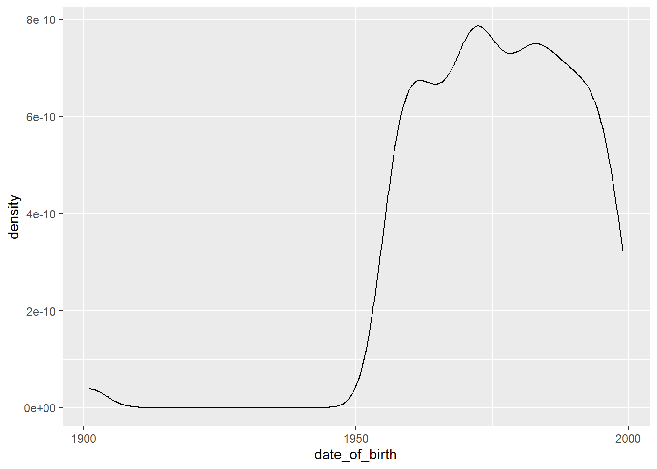
With a plot it is easy to see that there are a handful of birth dates around the year 1900, and then it takes off in the 1950s.
Here are some questions that we might want to explore further in the date_of_birth variable, after seeing the results of the summary() function and the plot:
- The earliest birth date is 1901-01-01. This would mean that the oldest staff member was 119 years old at 2020-01-01, the point at which the dataset was created. Perhaps you are already aware of the fact that only one person whose age has been independently verified lived long enough to celebrate their 120th birthday (they were 122 years, 164 days old when they passed away). 17 A possibility is that 1901-01-01 is a sentinel value, inserted as a placeholder for unknown or missing values. Further exploration will help our understanding; we can start with counting the number of cases for any particular date:
## # A tibble: 6 × 2
##   date_of_birth           n
##   <dttm>              <int>
## 1 1901-01-01 00:00:00    10
## 2 1955-10-26 00:00:00     2
## 3 1955-10-31 00:00:00     2
## 4 1955-11-22 00:00:00     2
## 5 1957-09-11 00:00:00     2
## 6 1958-10-28 00:00:00     2
There are 10 cases with the birth date entry of 1901-01-01. This is the sort of pattern we would see with a sentinel value.
Another approach to investigating this might be to derive a single year “age” variable from the date of birth, and visualize age using a box-and-whisker plot by one of the categorical variables to make outliers more apparent. We have a hunch that the “1901-01-01” sentinel value for date of birth might be associated with one category of occupation. Using our relational database “join” skills, we link the occupation variable from the “transaction” table and use occupation as a grouping variable in our plot. You’ll notice that the transaction table is not in a structure that suits our analysis needs, so we have to do some data wrangling first.
# step 1: read transaction table, which contains occupation
df_HR_transaction <-
  read_excel(
    path = dpjr::dpjr_data("cr25/cr25_human_resources.xlsx"),
    sheet = "df_HR_transaction",
    na = "NA"
  )

# step 2: determine occupation on the date the table was created
df_HR_occupation_2020 <- df_HR_transaction |>
  group_by(emp_id) |>
  summarize(occupation_current = max(occupation, na.rm = TRUE))

# step 3: in the main table calculate age and
#   join the occupation table created in step 2,
#   then plot the result
df_HR_main |>
  # calculate age on January 1, 2020
  mutate(age_2020 =
           date_of_birth %--% ymd("2020-01-01") %/% years(1)) |>
  # join the current occupation table
  left_join(df_HR_occupation_2020, by = "emp_id") |>
  # plot
  ggplot(aes(x = occupation_current, y = age_2020)) +
  geom_boxplot()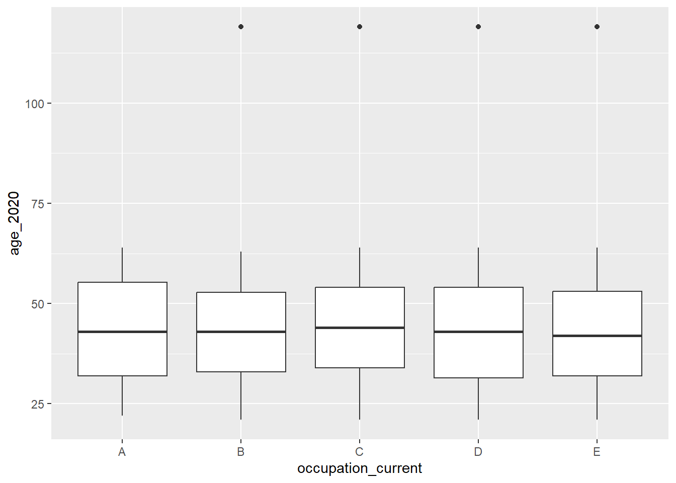
In the box-and-whisker visualization, we see that the sentinel values are in four of the five occupations, so the hunch was not correct.
11.3 Validation methods
While exploratory data analysis uses visualization and scans of data summaries to spot potentially dirty data, validation is a structured process of testing.
11.3.1 The {validate} package
As with other data analysis topics, people in the R user community have confronted the problem of dirty data and have written and shared functions to help the rest of us. The {validate} package M. van der Loo, Jonge, and Hsieh (2022) was written and is supported by methodologists at Statistics Netherlands, and provides tools for us to write structured validation tests.
The first function we will investigate in the package is check_that(), using the data in {palmerpenguins} (A. M. Horst, Hill, and Gorman 2022; A. Horst 2020). We know that the data in the package are nice and clean—they have already gone through a validation process.
Range of values:
We know, being experts on all things penguin, that gentoo penguins (Pygoscelis papua) are the third largest of the penguin species and can weigh up to 8.5 kg. So we might want to see if we have any records with penguins with a body mass of more than 8500 grams. The check_that() function inverts this question; we are ensuring that all of the records have penguin body mass values that are less than or equal to 8500 grams. If the value is below that value, it returns a “pass”.
The summary() function on the object that the check_that() function creates shows that all of the penguins have a body mass of less than or equal to 8500 grams, and there are 2 “NA” values in the data.
Relationship:
While the heaviest gentoo penguins can be up to 8.5 kg, it is very unusual to find an Adélie or chinstrap penguin that weighs more than 5 kg. What happens if we change the body mass threshold to 5000 grams?
In addition to telling us that there are 61 records where the value in the body_mass_g variable is greater than 5000 grams, it is also letting us know that there are 2 NA values.
We can add an if() statement that filters out the gentoo penguins, and then check the body mass.
check_penguins <- check_that(
  penguins,
  if (species != "Gentoo") body_mass_g <= 5000
  )

summary(check_penguins)
Now all the records (except the single “NA”) pass. What has happened? The first thing is that we have excluded all of the gentoo penguins—if it’s gentoo, it gets marked “pass”. All the remaining penguins (that is, the chinstrap and Adélie birds) are evaluated against the body mass value of 5000 grams. And they all pass.
Let’s explore the data a bit more. If we filter our penguins by those that are over 5000 grams, what do we find?
## # A tibble: 1 × 1
##   species
##   <fct>
## 1 Gentoo
So this is confirms that all of the heavier penguins are gentoos, meeting our expectations.
Range:
We know that the {palmerpenguin} data is from three seasons of measurement, 2007–2009. We can write a validation test to ensure that our year variable falls within that range.
##   name items passes fails nNA error warning
## 1   V1   344    344     0   0 FALSE   FALSE
##                                     expression
## 1 year - 2007 >= -1e-08 & year - 2009 <= 1e-08
What if we check for a single year?
##   name items passes fails nNA error warning                expression
## 1   V1   344    120   224   0 FALSE   FALSE abs(year - 2009) <= 1e-08
The output gives us the number of cases in that year in the column passes, and the number of cases that are not in that year in the column fails.
Relationship:
We know that some species have only been measured on one of the three islands. Gentoo penguins have only been sampled on Biscoe Island, and chinstrap penguins in our sample come only from Dream Island. Does the data reflect that?
In the first test (labelled g for gentoo), if it’s not a gentoo it gets included in the passes—and if it is a gentoo, it has to be on Biscoe Island to get a pass. In the c (for chinstrap) test, we will do the same for chinstrap penguins, which should all be on Dream Island.
check_penguins <-
  check_that(penguins,
             g = if (species == "Gentoo") island == "Biscoe",
             c = if (species == "Chinstrap") island == "Dream")

summary(check_penguins)
## name items passes fails nNA error warning
## 1 g 344 344 0 0 FALSE FALSE
## 2 c 344 344 0 0 FALSE FALSE
## expression
## 1 species != "Gentoo" | (island == "Biscoe")
## 2 species != "Chinstrap" | (island == "Dream")The output now includes the results of the two tests. Both tests have all of the cases pass, and none fail.
We could have written code to generate a summary table to check this. In many datasets, however, there will be too many combinations to reliably investigate in this manner.
## # A tibble: 5 × 3
## # Groups:   species [3]
##   species   island        n
##   <fct>     <fct>     <int>
## 1 Adelie    Biscoe       44
## 2 Adelie    Dream        56
## 3 Adelie    Torgersen    52
## 4 Chinstrap Dream        68
## 5 Gentoo    Biscoe      124
A single check_that() test could be written using the “AND” operator &.
check_penguins <-
  check_that(penguins,
             if (species == "Gentoo") island == "Biscoe" &
             if (species == "Chinstrap") island == "Dream")
We can also test against a defined list. This strategy can be useful if there is an extensive list against which we need to evaluate our data. Imagine checking the spellings of every city and town in the region where you live. If you have a pre-defined list of those names in an existing data file, that list can be read into your R environment, and the test run against that list. In this short example, an object called island_list is created, and the validation check is run against the contents of that list.
island_list <- c("Biscoe", "Dream", "Torgersen")

check_penguins <-
  check_that(penguins,
             if (species == "Adelie") island %in% island_list)

summary(check_penguins)
## name items passes fails nNA error warning
## 1 V1 344 344 0 0 FALSE FALSE
## expression
## 1 species != "Adelie" | (island %vin% island_list)What happens if we fail to include Dream Island in our list of islands where Adélie penguins are found?
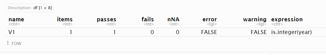
The {validator} also allows us to check variable types within our check_that() function. Because R stores a dataframe column as a single type, this returns only one pass/fail evaluation.
11.3.2 badpenguins
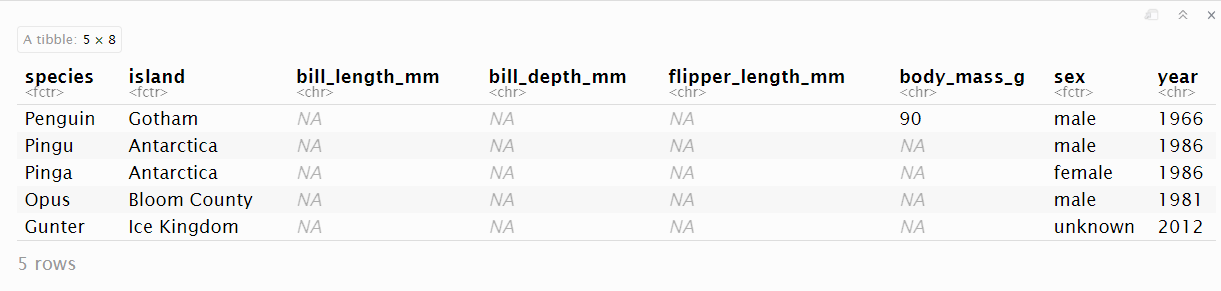
The “badpenguins.rds” file adds five fictional penguins to the original “penguins” table, including measurement data. Let’s load the data file “badpenguins.rds” (an R data file) and run a couple of the tests we used earlier:
## # A tibble: 6 × 8
##   species island bill_length_mm bill_depth_mm flipper_length_mm body_mass_g
##   <fct>   <fct>  <chr>          <chr>         <chr>             <chr>
## 1 Chinst… Dream  50.2           18.7          198               3775
## 2 Penguin Gotham <NA>           <NA>          <NA>              90
## 3 Pingu   Antar… <NA>           <NA>          <NA>              <NA>
## 4 Pinga   Antar… <NA>           <NA>          <NA>              <NA>
## 5 Opus    Bloom… <NA>           <NA>          <NA>              <NA>
## 6 Gunter  Ice K… <NA>           <NA>          <NA>              <NA>
## # ℹ 2 more variables: sex <fct>, year <chr>## name items passes fails nNA error warning expression
## 1 V1 349 344 5 0 FALSE FALSE year >= 2007 & year <= 2009## name items passes fails nNA error warning expression
## 1 V1 349 344 5 0 FALSE FALSE island %vin% island_listIn both cases, we get 5 “fails”.
11.3.3 Investigating the fails
How can we check which records have failed?
{validate} provides two other functions, validator() and confront(), which give us a way to
run multiple checks at a time, and
generate a detailed record-by-record account of which records have failed our test.
First, we assign the syntax of our tests using validator() to an object “penguin_tests”.
penguin_tests <- validator(
  island %in% island_list,
  year >= 2007 & year <= 2009,
  body_mass_g <= 8500
)

penguin_tests
## Object of class 'validator' with 3 elements:
## V1: island %in% island_list
## V2: year >= 2007 & year <= 2009
## V3: body_mass_g <= 8500In the next step, we apply those tests in a sequence of “confrontations” using the confront() function, generating an output object that we can investigate.
## Object of class 'validation'
## Call:
##     confront(dat = badpenguins, x = penguin_tests)
##
## Rules confronted: 3
##    With fails   : 3
##    With missings: 1
##    Threw warning: 0
## Threw error : 0## name items passes fails nNA error warning expression
## 1 V1 349 344 5 0 FALSE FALSE island %vin% island_list
## 2 V2 349 344 5 0 FALSE FALSE year >= 2007 & year <= 2009
## 3 V3 349 342 1 6 FALSE FALSE body_mass_g <= 8500Let’s look at the last ten rows of the results of the confront() function of our badpenguins data. Rows 340 through 344 are original to the clean penguins dataset; 345 through 349 are the bad penguins. The first of the bad penguins fails on all three tests, while the others fail on the first two and have “NA” values for the third.
##           V1    V2    V3
## [340,]  TRUE  TRUE  TRUE
## [341,]  TRUE  TRUE  TRUE
## [342,]  TRUE  TRUE  TRUE
## [343,]  TRUE  TRUE  TRUE
## [344,]  TRUE  TRUE  TRUE
## [345,] FALSE FALSE FALSE
## [346,] FALSE FALSE    NA
## [347,] FALSE FALSE    NA
## [348,] FALSE FALSE    NA
## [349,] FALSE FALSE    NA
In this example, our prior knowledge of the data gives us the insight to quickly target the rows that failed the validation tests. In the real world, filtering the object that results from our validation tests will allow us to identify the rows that contain the records that fail the tests.
The function we use for this is violating(). The two arguments in the violating() function are
the original data frame
badpenguinsandthe object that resulted from the
confront()function,penguin_confront.
Now that we know the details of the cases that have failed the test, we can make some decisions—based on our understanding of the research we are undertaking—about how to deal with these cases.