Chapter 5 Importing data: plain-text files
In this chapter:
Importing data from delimited text files
Importing data from fixed-width text files
5.1 Delimited plain-text files
Plain-text files (sometimes called “ASCII files”, after the character encoding standard they use) are often used to share data. They are limited in what they can contain, which has both downsides and upsides. On the downside, they can’t carry any additional information with them, such as variable types and labels. But on the upside, they don’t carry any additional information that requires additional interpretation by the software. This means they can be read consistently by a wide variety of software tools.
Plain-text files come in two varieties: delimited and fixed-width. “Delimited” is a reference to the fact that the files have a character that marks the boundary between two variables. A very common delimited format is the CSV file; the letters in the file name stand for “Comma Separated Values”, and use a comma as the variable delimiter. Another delimited type, somewhat less common, uses the tab character to separate the variables, and will have the extension “TSV” for, you guessed it, “Tab Separated Values”. Occasionally you will find files that use semi-colons, colons, or spaces as the delimiters.
There are base R functions to read this type of file. The functions within the {readr} (Wickham and Hester 2020) package has some advantages over the base R functions when it comes to plain-text files. (The {readr} package is part of the tidyverse.) Compared to the equivalent base R functions, the {readr} functions are quite a bit faster, and the package’s functions provide some useful flexibility when it comes to defining variable types as part of the read operation (rather than reading in the dat and then altering the variable types). As well, it returns a tibble instead of a dataframe. (For information about the difference, see (Wickham 2019a, 3.6 Data frames and tibbles). For working with very large files, you may want to investigate the fread() function in the {data.table} package(Dowle et al. 2023).)
We activate {readr} by using the library() function:
In this chapter, we will be using two of the {readr} functions. Each has a variety of arguments that allow us to control the behaviour of the function; those will be dealt with in the examples.
| function | purpose |
|---|---|
read_csv() |
reads the contents of a CSV file |
read_fwf() |
reads the contents of a fixed-width text file |
5.2 Using {readr} to read a CSV file
In the following examples, we will use versions of the data in the {palmerpenguins} data (A. M. Horst, Hill, and Gorman 2022; A. Horst 2020)
In the code chunks below, an R character string object penguins_path is created that contains the text string with the location of the file “penguins.csv”.
In the first example, the file has been loaded to our computer using the {dpjr} package, and uses the dpjr_data() function from that package to access the file (no matter its location on our computer).
In the second example, the file is located in a directory called “data” that is in our RStudio project folder. The {here} package will generate the full path, with slash or backslash separators (depending on your computer’s operating system), starting at the location of the RStudio project.
The penguins_path object is then used in the function read_csv() to create a dataframe object called penguins_data.
# Example 2
# create object path using the {here} package
penguins_path <- here::here("data", "penguins.csv")

# read the contents of the CSV file
penguins_data <- read_csv(penguins_path)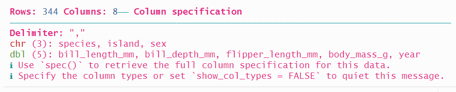
The function returns a message letting us know the type that each variable is assigned.
The arguments of the {readr} package allow a lot of control over how the file is read. Of particular utility are the following:
| argument | purpose |
|---|---|
col_types = cols() |
define variable types |
na = "" |
specify which values you want to be turned into NA |
skip = 0 |
specify how many rows to skip; the default is 0 |
n_max = Inf |
the maximum number of records to read; the default is Inf for infinity, interpreted as the last row of the file |
Adding the col_types = cols() parameter has two benefits. First, defining the variable type avoids errors (such as numeric fields will be read as such, and not as characters) and speeds up the read process since R doesn’t have to check and infer the variable type.
Second, it allows us to alter what {readr} has decided for us. For example, we could set the species variable to be a factor type variable.
When we show the entire table, we can see that the variable species is now a factor type.
## # A tibble: 344 × 8
##    species island    bill_length_mm bill_depth_mm
##    <fct>   <chr>              <dbl>         <dbl>
##  1 Adelie  Torgersen           39.1          18.7
##  2 Adelie  Torgersen           39.5          17.4
##  3 Adelie  Torgersen           40.3          18
##  4 Adelie  Torgersen           NA            NA
##  5 Adelie  Torgersen           36.7          19.3
##  6 Adelie  Torgersen           39.3          20.6
##  7 Adelie  Torgersen           38.9          17.8
##  8 Adelie  Torgersen           39.2          19.6
##  9 Adelie  Torgersen           34.1          18.1
## 10 Adelie  Torgersen           42            20.2
## # ℹ 334 more rows
## # ℹ 4 more variables: flipper_length_mm <dbl>,
## #   body_mass_g <dbl>, sex <chr>, year <dbl>
If we were working with a very large file and wanted to read the first five rows, just to see what’s there, we could use the n_max = argument:
## # A tibble: 5 × 8
##   species island    bill_length_mm bill_depth_mm
##   <chr>   <chr>              <dbl>         <dbl>
## 1 Adelie  Torgersen           39.1          18.7
## 2 Adelie  Torgersen           39.5          17.4
## 3 Adelie  Torgersen           40.3          18
## 4 Adelie  Torgersen           NA            NA
## 5 Adelie  Torgersen           36.7          19.3
## # ℹ 4 more variables: flipper_length_mm <dbl>,
## #   body_mass_g <dbl>, sex <chr>, year <dbl>
5.3 Fixed-width files
Fixed-width files don’t use a delimiter, and instead specify which column(s) each variable occupies, consistently for every row in the entire file.
Fixed-width files are a hold-over from the days when storage was expensive and/or on punch cards. This meant that specific columns in the table (or card) were assigned to a particular variable, and precious space was not consumed with a delimiter. Compression methods have since meant that a CSV file with unfixed variable lengths is more common, but in some big data applications, fixed-width files can be much more efficient.
If you ever have to deal with a fixed-width file, you will (or should!) receive a companion file letting you know the locations of each variable in every row.
In this example, we will use the one provided in the {dpjr} package, “authors_fwf.txt”. This code chunk assigns the path to the file location, which we can use in our code later.
This simple file has four (or as we will see, sometimes three, if we combine first and last name as one) variables, and three records (or rows).
first name
last name
U.S. state of birth (two-letter abbreviation)
randomly generated unique ID
If we open the file in a text editor, we see this:
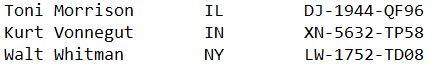
We could also use the {base R} function readLines() to see the lines:
## [1] "Toni Morrison       IL        DJ-1944-QF96"
## [2] "Kurt Vonnegut       IN        XN-5632-TP58"
## [3] "Walt Whitman        NY        LW-1752-TD08"
The arguments within the readr::read_fwf() function include those listed above for the read_csv() function, and some others that are specific to fixed-width files.
| argument | purpose |
|---|---|
col_names = c() |
defines a list of the names for the variables |
fwf_widths(widths = c(), col_names = c()) |
a list of the character length of each variable, and their names |
fwf_positions(start = , end = , col_names = c()) |
character position of the start and end of each variable, and their names |
fwf_cols(variable1_name = c(), variable2_name = c()) |
name followed by start and end position of each variable) |
fwf_cols(variable1_name = width, variable2_name = width) |
name followed by width of each variable) |
The examples below will elaborate on these arguments.
The first approach would be to allow {readr} to guess where the column breaks are. The fwf_empty() function looks through the specified file and returns the beginning and ending locations it has guessed, as well as the skip value that the read_fwf() function uses.
Note that the column names are specified in a list.
## $begin
## [1] 0 5 20 30
##
## $end
## [1] 4 13 22 NA
##
## $col_names
## [1] "first" "last" "state" "unique_id"That information can then be used by the read_fwf() function:
read_fwf(authors_path,
fwf_empty(
  authors_path,
  col_names = c("first", "last", "state", "unique_id")
))## # A tibble: 3 × 4
## first last state unique_id
## <chr> <chr> <chr> <chr>
## 1 Toni Morrison IL DJ-1944-QF96
## 2 Kurt Vonnegut IN XN-5632-TP58
## 3 Walt Whitman NY LW-1752-TD08Note that {readr} will impute the variable type, as it did with the CSV file. And although we won’t implement it in these examples, in the same way read_fwf() allows us to use the col_types specification, as well as na, skip, and others. See the read_fwf() reference at https://readr.tidyverse.org/reference/read_fwf.html for all the details.
Reading this fixed-width file with these three author names worked, but it could break quite easily. We just need one person with three or more components to their name (initials, spaces, or hyphens, as in Ursula K. Le Guin or Ta-Nehisi Coates), or some missing values, and the inconsistent structure throws off the read_fwf() parser.
In the following example, we read a longer list of author names:
authors2_path <- dpjr::dpjr_data("authors2_fwf.txt")

fwf_empty(authors2_path,
          col_names = c("first", "last", "state", "unique_id"))
## $begin
## [1] 0 20 30
##
## $end
## [1] 19 22 NA
##
## $col_names
## [1] "first" "last" "state" "unique_id"The fwf_empty() function found only three columns, as shown in the “begin” and “end” values that are returned.
When we use the read function, it finds three columns:
## # A tibble: 10 × 3
##    X1                  X2    X3
##    <chr>               <chr> <chr>
##  1 Toni Morrison       IL    DJ-1944-QF96
##  2 Kurt Vonnegut       IN    XN-5632-TP58
##  3 Walt Whitman        NY    LW-1752-TD08
##  4 Ursula K. Le Guin   CA    EZ-9789-EA77
##  5 Ta-Nehisi Coates    NY    YN-5151-NV82
##  6 W. E. B. Du Bois    MA    HN-6134-NF80
##  7 F. Scott Fitzgerald MN    YH-4405-TR02
##  8 N.K. Jemisin        IA    EF-7340-DW20
##  9 Flannery O'Connor   GA    HB-8269-XC88
## 10 Henry David Thoreau MA    RL-8200-SU83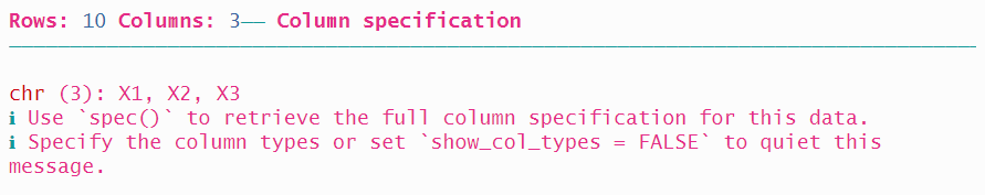
Adding the col_names = argument now mis-identifies the variables.
read_fwf(authors2_path,
         fwf_empty(
           authors2_path,
           col_names = c("first", "last", "state", "unique_id")
         ))
## # A tibble: 10 × 3
## first last state
## <chr> <chr> <chr>
## 1 Toni Morrison IL DJ-1944-QF96
## 2 Kurt Vonnegut IN XN-5632-TP58
## 3 Walt Whitman NY LW-1752-TD08
## 4 Ursula K. Le Guin CA EZ-9789-EA77
## 5 Ta-Nehisi Coates NY YN-5151-NV82
## 6 W. E. B. Du Bois MA HN-6134-NF80
## 7 F. Scott Fitzgerald MN YH-4405-TR02
## 8 N.K. Jemisin IA EF-7340-DW20
## 9 Flannery O'Connor GA HB-8269-XC88
## 10 Henry David Thoreau MA RL-8200-SU83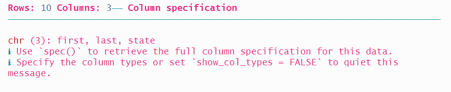
A more reliable approach is to specify exactly the width of each column. Note that in the example below, we specify only “name” without splitting it into first and last.
The variables and their widths are as follows:
| variable | width | start position | end position |
|---|---|---|---|
| name | 20 | 1 | 20 |
| state | 10 | 21 | 30 |
| uniqueID | 12 | 31 | 42 |
The widths of each column can be added using the fwf_widths argument:
read_fwf(authors2_path,
         fwf_widths(widths = c(20, 10, 12),
                    col_names = c("name", "state", "unique_id")))
## # A tibble: 10 × 3
## name state unique_id
## <chr> <chr> <chr>
## 1 Toni Morrison IL DJ-1944-QF96
## 2 Kurt Vonnegut IN XN-5632-TP58
## 3 Walt Whitman NY LW-1752-TD08
## 4 Ursula K. Le Guin CA EZ-9789-EA77
## 5 Ta-Nehisi Coates NY YN-5151-NV82
## 6 W. E. B. Du Bois MA HN-6134-NF80
## 7 F. Scott Fitzgerald MN YH-4405-TR02
## 8 N.K. Jemisin IA EF-7340-DW20
## 9 Flannery O'Connor GA HB-8269-XC88
## 10 Henry David Thoreau MA RL-8200-SU83A third option is to provide two lists of locations using fwf_positions(), the first with the start positions, and the second with the end positions. The first variable name starts at position 1 and ends at position 20, and the second variable unique_id starts at 30 and ends at 42. Note that we won’t read the state variable which occupies the ten columns from 21 through 30.
read_fwf(authors2_path,
fwf_positions(start = c(1, 31), end = c(20, 42),
col_names = c("name", "unique_id")))## # A tibble: 10 × 2
## name unique_id
## <chr> <chr>
## 1 Toni Morrison DJ-1944-QF96
## 2 Kurt Vonnegut XN-5632-TP58
## 3 Walt Whitman LW-1752-TD08
## 4 Ursula K. Le Guin EZ-9789-EA77
## 5 Ta-Nehisi Coates YN-5151-NV82
## 6 W. E. B. Du Bois HN-6134-NF80
## 7 F. Scott Fitzgerald YH-4405-TR02
## 8 N.K. Jemisin EF-7340-DW20
## 9 Flannery O'Connor HB-8269-XC88
## 10 Henry David Thoreau RL-8200-SU83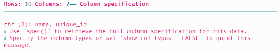
The fourth option is a syntactic variation on the third, with the same values but in a different order. This time, all of the relevant information about each variable is aggregated, with the variable name followed by the start and end locations.
## # A tibble: 10 × 2
## name unique_id
## <chr> <chr>
## 1 Toni Morrison DJ-1944-QF96
## 2 Kurt Vonnegut XN-5632-TP58
## 3 Walt Whitman LW-1752-TD08
## 4 Ursula K. Le Guin EZ-9789-EA77
## 5 Ta-Nehisi Coates YN-5151-NV82
## 6 W. E. B. Du Bois HN-6134-NF80
## 7 F. Scott Fitzgerald YH-4405-TR02
## 8 N.K. Jemisin EF-7340-DW20
## 9 Flannery O'Connor HB-8269-XC88
## 10 Henry David Thoreau RL-8200-SU83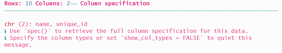
And finally, {readr} provides a fifth way to read in a fixed-width file that is a variation on the second approach we saw, with the name and the width values aggregated.
## # A tibble: 10 × 3
##    name                state unique_id
##    <chr>               <chr> <chr>
##  1 Toni Morrison       IL    DJ-1944-QF96
##  2 Kurt Vonnegut       IN    XN-5632-TP58
##  3 Walt Whitman        NY    LW-1752-TD08
##  4 Ursula K. Le Guin   CA    EZ-9789-EA77
##  5 Ta-Nehisi Coates    NY    YN-5151-NV82
##  6 W. E. B. Du Bois    MA    HN-6134-NF80
##  7 F. Scott Fitzgerald MN    YH-4405-TR02
##  8 N.K. Jemisin        IA    EF-7340-DW20
##  9 Flannery O'Connor   GA    HB-8269-XC88
## 10 Henry David Thoreau MA    RL-8200-SU83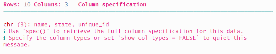
5.3.1 An extreme example of a fixed-width file
A particularly interesting research question is the relationship between education level and different health outcomes. In this example, we will start the process of importing a large file that contains data that will allow us to explore whether there is a correlation.
Statistics Canada has made available a Public-Use Microdata File (PUMF) of the Joint Canada/United States Survey of Health (JCUSH), a telephone survey conducted in late 2002 and early 2003. There were 8,688 respondents to the survey, 3,505 Canadians and 5,183 Americans. The data file that is available is anonymized, so we have access to the individual responses, which will facilitate additional analysis.
The webpage for the survey, including the PUMF file, data dictionary, and methodological notes, is here: https://www150.statcan.gc.ca/n1/pub/82m0022x/2003001/4069119-eng.htm
The PUMF is a fixed-width file named “JCUSH.txt”. This file is quite a lot larger than the author names example above. There are the 8,688 records, one for each survey respondent. The data also consists of 366 variables, a combination of assigned variables (such as the unique respondent identification number and the country), survey question responses, and derived variables that are calculated as part of the post-survey data processing.
Here’s what the first 40 characters of the first record looks like:
## [1] "1000033308351200211170432144421333431126"There’s not a bit of white space anywhere in this data file. The 366 variables are stored in only 552 columns—an average of 1.5 columns per variable! This is a good example of the efficiency associated with this approach to encoding the data.
Let’s imagine that our research goal is to determine if there is a relationship between a person’s level of education and their health outcomes. We’ve reviewed the data documentation, and it is clear that the JCUSH data has what we need.
Here’s how one variable, highest level of post-secondary education achieved, appears in the data dictionary:
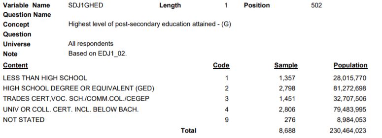
The variable SDJ1GHED is 1 character long, in position 502 of the data. The variable might be only 1 character long, but when coupled with the information in the Content table, it becomes a very powerful piece of information.
For our analysis question, we will read in four variables: the unique household identification number, the country, the overall health outcomes, and education level. For the variable names, we will use the same ones used in the data dictionary:
| name | variable | length | position |
|---|---|---|---|
| SAMPLEID | Household identifier | 12 | 1 - 12 |
| SPJ1_TYP | Sample type [country] | 1 | 13 |
| GHJ1DHDI | Health Description Index | 1 | 32 |
| SDJ1GHED | Highest level of post-secondary education attained | 1 | 502 |
You will note in the code below that in the case of the variables that are of length “1”, the value to indicate the start and end positions are the same.
As well, the SAMPLEID variable is a 12-digit number; the read_fwf() function will interpret this as variable type double, and represent it in scientific notation. To be useful, we want to be able to see and evaluate the entire string. As a result, we use col_types() to specify SAMPLEID as a character.
jcush <- readr::read_fwf(dpjr::dpjr_data("JCUSH.txt"),
         fwf_cols(
           SAMPLEID = c(1, 12),
           SPJ1_TYP = c(13, 13),
           GHJ1DHDI = c(32, 32),
           SDJ1GHED = c(502, 502)
           ),
         col_types = list(
           SAMPLEID = col_character()
         ))

head(jcush)
## # A tibble: 6 × 4
## SAMPLEID SPJ1_TYP GHJ1DHDI SDJ1GHED
## <chr> <dbl> <dbl> <dbl>
## 1 100003330835 1 3 4
## 2 100004903392 1 3 2
## 3 100010137168 1 2 1
## 4 100010225523 1 3 3
## 5 100011623697 1 2 2
## 6 100013652729 1 4 3Imagine, though, the challenge of handling this amount of data at one time! Between the many variables and the complex value labels, the “data” is more than just the fixed-width file. This is a circumstance where a different data storage solution (as we will see later) has some strengths.