Chapter 10 Linking to relational databases
In this chapter:
Importing data directly from relational databases (SQL)
Using relational data as part of the data preparation workflow
10.1 Relational data
Relational databases are commonly used for data storage. Unlike a “flat file” which contains all of the variables, the data is stored in multiple tables, which are linked via common variables (known as the “keys”). This facilitates efficient storage, as information does not need to be duplicated in multiple rows. We have seen an example of a relational table earlier, where we built a concordance table for the administrative geography of England and Wales in 6.
In that example, all of the data was loaded into our computer’s memory. In other instances, the size of the database, across multiple tables, will be such that it exceeds the capacity of your computer. In those cases, a server-based database will be established, and as the data analyst, we will need to retrieve only the variables and records that we need for our work. A database query can also include the calculation of summary statistics, which shifts the computational load to the server.
While SQL is the most commonly used query language, there are R packages that allow us to
Connect to a database,
Write the code for our queries in R,
Run the query, and
Do our work in an R environment.
Writing your code in an R Markdown or Quarto document also gives you the flexibility to write the code in SQL, if that’s your preferred approach.
This exercise replicates the joins described in the “Relational data” chapter of R for Data Science by Hadley Wickham & Garrett Grolemund (Wickham and Grolemund 2016). Instead of using the R {nycflights13} package (Wickham and RStudio 2021), we will use a SQLite version of the same database.
In this database, there are five separate tables. The table flights in the database contains all 336,776 flights that departed from New York City in 2013. The data comes from the US Bureau of Transportation Statistics and is documented in ?flights
The other tables in the database are:
airlineslets you look up the full carrier name from its abbreviated code,airportsgives information about each airport, identified by thefaaairport code,planesgives information about each plane, identified by itstailnum,weathergives the weather at each NYC airport for each hour.
The tables are related to flights by the fact that they have variables in common. These are known as the “key” variables.
This diagram shows the relationships:
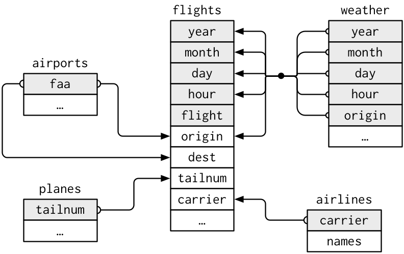
(From (Wickham and Grolemund 2016), p.174)
10.1.1 Connect to the database
SQL is a language widely used to manipulate and extract data in relational databases. As a consequence, there are many relational databases built in this format. Most often, these databases will be housed on a network server, but for smaller databases, you might install the file on your computer.
In R, we can use the package {dbplyr} (Wickham et al. 2023) to access SQL databases and SQL functions. In addition, we need {DBI} (Müller 2022) and {RSQLite} (Müller et al. 2023) to establish the connection to the RSQLite database.
The code below establishes the connection to the database and assigns the connection (not the data table!) to the object con_nycf (for “Connection to New York City Flights”). You will note that the {RSQLite} function SQLite() is inside the {DBI} function dbConnect(). The {DBI} package supports a wide range of different database types, including the widely-used MySQL and Postgres.
# establish the connection to the database file
con_nycf <-
  DBI::dbConnect(RSQLite::SQLite(), "data/nycflights13_sql.sqlite")

# list the tables in the connected database
dbListTables(con_nycf)
## [1] "airlines" "airports" "flights" "planes"
## [5] "sqlite_stat1" "sqlite_stat4" "weather"Now that we have a connection to the database, we can establish a connection to a particular table, using the {dplyr} function tbl(). Note that the flights object is not the table but is the connection to the table.
10.1.2 Submit queries
With the object “flights” now established in our environment, we can write R code to create a subset of the flights—those that went to Seattle. Again, the flights_SEA object is not a dataframe, but a set of instructions that creates the connection and the query.
We can also use the show_query() function of {dbplyr} to generate the SQL translation of the R code:
## <SQL>
## SELECT `flights`.*
## FROM `flights`
## WHERE (`dest` = 'SEA')
In SQL, we use SELECT to select the columns (or variables) we want (you will note this is the same term as {dplyr}). The asterisk “*” is a wildcard to select all the tables.
FROM indicates which table from which we want to draw the columns.
And finally, the filtering by city uses the SQL function WHERE.
In the code below, we create a summary table of the average flight time from New York to Seattle, by airline.
SEA <- flights_SEA |>
  select("month", "carrier", "air_time") |>
  group_by(carrier) |>
  summarize(
    n = n(),
    min_air_time = min(air_time),
    mean_air_time = mean(air_time),
    max_air_time = max(air_time)) |>
  # enter the resulting table into the R environment
  collect()

SEA
## # A tibble: 5 × 5
## carrier n min_air_time mean_air_time max_air_time
## <chr> <int> <dbl> <dbl> <dbl>
## 1 AA 365 289 336. 385
## 2 AS 714 277 326. 392
## 3 B6 514 283 330. 378
## 4 DL 1213 275 327. 389
## 5 UA 1117 280 326. 39410.1.3 Using SQL in your R code
In addition to writing native R code, we can embed SQL inside R code. In the example below, an R chunk in the R Markdown document has R code that uses the dbSendQuery() function. Inside this function, we first name the connection we are using and then inside the quotation marks write SQL code: "SELECT * FROM flights WHERE dest = 'SEA'".
This query instruction gets saved as the object SEA_sql.
The R chunk then has a second line that uses the dbFetch() function to run the SQL query.
Both the dbSendQuery() and dbFetch() are functions from the {DBI} package.
10.2 Running SQL language chunks in R Markdown
The book R Markdown: The Definitive Guide (Xie, Allaire, and Grolemund 2019, chap. 2.7.3) provides instructions on how to set up your R Markdown in RStudio so that you can run SQL language chunks, including using SQLite.
Once this has been done, our R Markdown document can incorporate native SQL queries into the workflow. Note that in our SQL chunk, we specify the connection. As we continue to work through this example, this is the con_nycf object created earlier. The start of our SQL code chunk would contain this text:
{sql, connection=con_nycf}
10.2.1 Mutating joins and summary tables
A mutating join is one that combines variables from two tables, based on matching observations on keys.
In this R code, we create a summary table of the flights that went from New York to Seattle, by the name of the airline. The full airline name is not in the flights table; to get that, we need to join the airline name from the airlines table to the Seattle summary of the flights table.
The first step is to establish a connection to the airlines table.
Once the connection is made the tables can be joined using the left_join() function from {dplyr}, the grouped summary calculation made, and the table sorted from most to least frequent number of flights.
The table is also formatted for publication using the {gt} package (Iannone et al. 2023); the core gt() function is the first step, and many other formatting options are possible with this package.
# join and summary table
flights_SEA_summary <- flights_SEA |>
#  select(-origin, -dest) |>
  left_join(airlines, by = "carrier") |>
  group_by(name) |>
  tally() |>
  arrange(desc(n))

flights_SEA_summary |>
gt()| name | n |
|---|---|
| Delta Air Lines Inc. | 1213 |
| United Air Lines Inc. | 1117 |
| Alaska Airlines Inc. | 714 |
| JetBlue Airways | 514 |
| American Airlines Inc. | 365 |
The SQL code below returns the same table. We can see one difference in how the code is written—it runs “inside out” with the third step coming before the first and second, rather than in the linear manner we are accustomed to in our R pipes.
-- 3. select `name` variable from joined table and apply count
SELECT `name`, COUNT(*) AS `n`
FROM (
  SELECT `flights_sea`.*, `name`
-- 1. query to filter Seattle flights
  FROM (
    SELECT *
    FROM `flights`
    WHERE (`dest` = 'SEA')
  ) AS `flights_sea`
-- 2. join to airlines table
  LEFT JOIN `airlines`
    ON (`flights_sea`.`carrier` = `airlines`.`carrier`)
)
-- 4. define grouping for COUNT (from step 3) and sort
GROUP BY `name`
ORDER BY `n` DESC| name | n |
|---|---|
| Delta Air Lines Inc. | 1213 |
| United Air Lines Inc. | 1117 |
| Alaska Airlines Inc. | 714 |
| JetBlue Airways | 514 |
| American Airlines Inc. | 365 |
The joins are named using terms similar to those you are familiar with from {dplyr}. This left join will return all of the records from the flights table, and the variables from airlines where there is a match.
To indicate the key variable for the join, we use the SQL term ON. Note that we specify the table and the variable, separated by a period.
For more information on using SQL, with a focus on SQLite, Thomas Nield’s Getting Started with SQL (Nield 2016) is highly recommended.
10.3 Using the {tidylog} package
An important element of any table join is to check the result, to see if it conforms to our expectations. The {tidylog} package (Elders and Oldoni 2020)
The authors of the package acknowledge that the functionality adds some computational and time overhead to the processing, but this may be worth the cost. Judiciously used, the information it returns can give an immediate indication if the code has worked. This is particularly true in the early stages of writing your code—the functions can be removed when you are confident you are getting the results you expect.
After running the library(tidylog) function, the results are automatically generated.
The Major League Baseball teams play in cities in the United States and Canada (currently only Toronto!), but draw the best players from around the world. In this example the code creates a summary table to show the country of birth of the player who batted in the 2001 season.
For this we will use the data stored in the R package that contains the Lahman baseball database (named after Sean Lahman, the person who initially created the database) (Friendly et al. 2020).
At the completion of this run, the {tidylog} package produces some summary information about the join, the grouping, and the tally functions.
## start with the Batting table
Lahman::Batting |>
  ## filter for year
  filter(yearID == "2001") |>
  ## join to People table (where the birth country is recorded)
  left_join(Lahman::People, by = "playerID") |>
  ## now group_by and tally
  group_by(birthCountry) |>
  tally() |>
  arrange(desc(n)) |>
  slice_head(n = 10)
## # A tibble: 10 × 2
## birthCountry n
## <chr> <int>
## 1 USA 1002
## 2 D.R. 120
## 3 P.R. 57
## 4 Venezuela 54
## 5 Mexico 19
## 6 Cuba 16
## 7 CAN 14
## 8 Japan 14
## 9 Panama 11
## 10 Australia 6