Chapter 12 Cleaning techniques
In this chapter:
Cleaning dates and strings
Creating conditional and calculated variables
- indicator variables (also known as dummy variables (Suits 1957) and “one hot” encoding)
Dealing with missing values
12.1 Introduction
We have already applied some cleaning methods. In the chapters on importing data, we tackled a variety of techniques that would fall into “data cleaning,” including assigning variable types and restructuring data into a tidy format. In this chapter, we look in more depth at some examples of recurring data cleaning challenges.
12.2 Cleaning dates
A recurring challenge in many data analysis projects is to deal with date and time fields. One of the first steps of any data cleaning project should be to ensure that these are in a consistent format that can be easily manipulated.
As we saw in (Broman and Woo 2017), there is an international standard (ISO 8601) for an unambiguous and principled way to write dates and times (and in combination, date-times). For dates, we write YYYY-MM-DD. Similarly, time is written T[hh][mm][ss] or T[hh]:[mm]:[ss], with hours (on a 24-hour clock) followed by minutes and seconds.
When we are working with dates, the objective of our cleaning is to transform the date into the ISO 8601 standard and then, where appropriate, transform that structure into a date type variable. The benefits of the date type format are many, not the least of which are the R tools built to streamline analysis and visualization that use date type variables, (Wickham, Çetinkaya-Rundel, and Grolemund 2023, chap. 18) and those same tools allow us to tackle cleaning variables that capture date elements.
One such package is {lubridate}, part of the tidyverse.
12.2.1 Creating a date-time field
The first way that dates might be represented in your data is as three separate fields, one for year, one for month, and one for day. These can be assembled into a single date variable using the make_date(), or a single datetime variable using make_datetime().
In the {Lahman}(Friendly et al. 2020) table “People”, each player’s birth date is stored as three separate variables. They can be combined into a single variable using make_date():
Lahman::People |>
  slice_head(n = 10) |>
  select(playerID, birthYear, birthMonth, birthMonth, birthDay) |>
  # create date-time variable
   mutate(birthDate = make_datetime(birthYear, birthMonth, birthDay))
## playerID birthYear birthMonth birthDay birthDate
## 1 aardsda01 1981 12 27 1981-12-27
## 2 aaronha01 1934 2 5 1934-02-05
## 3 aaronto01 1939 8 5 1939-08-05
## 4 aasedo01 1954 9 8 1954-09-08
## 5 abadan01 1972 8 25 1972-08-25
## 6 abadfe01 1985 12 17 1985-12-17
## 7 abadijo01 1850 11 4 1850-11-04
## 8 abbated01 1877 4 15 1877-04-15
## 9 abbeybe01 1869 11 11 1869-11-11
## 10 abbeych01 1866 10 14 1866-10-14The second problematic way dates are stored is in a variety of often ambiguous sequences. This might included text strings for the month (for example “Jan”, “January”, or “Janvier” rather than “01”), two-digit years (does “12” refer to 2012 or 1912?), and ambiguous ordering of months and days (does “12” refer to the twelfth day of the month or December?)
If we know the way the data is stored, we can use {lubridate} functions to process the data into YYYY-MM-DD. These three very different date formats can be transformed into a consistent format:
## [1] "1973-10-22"## [1] "1973-10-22"## [1] "1973-10-22"A third manner in which dates can be stored is with a truncated representation. For example, total sales for the entire month might be recorded as a single value associated with “Jan 2017” or “2017-01”, or a quarterly measurement might be “2017-Q1”.
## [1] "1973-10-01"## [1] "1973-10-01"## [1] "1973-01-01"If we have a variable with annual data, we have to use the parameter truncated = to convert our year into a date format:
## [1] "1973-01-01"By mutating these various representations into a consistent YYYY-MM-DD format, we can now run calculations. In the example below, we calculate the average size of the Canadian labour force in a given year:
First, we transform the character variable REF_DATE into a date type variable.
With the variable in the date type, we can use functions within {lubridate} for our analysis.
To calculate the average employment in each year:
## # A tibble: 4 × 2
##   `year(REF_DATE)` `mean(VALUE)`
##              <dbl>         <dbl>
## 1             2011        17244.
## 2             2012        17476.
## 3             2013        17712.
## 4             2014        17783.
For the second analysis, we might be interested in determining if there is any seasonality in the Canadian labour force:
## # A tibble: 12 × 2
##    `month(REF_DATE)` `mean(VALUE)`
##                <dbl>         <dbl>
##  1                 1        17841.
##  2                 2        17960.
##  3                 3        17907.
##  4                 4        17848.
##  5                 5        18255.
##  6                 6        18539.
##  7                 7        18514.
##  8                 8        18514.
##  9                 9        18423.
## 10                10        18458.
## 11                11        18421.
## 12                12        18369.
12.3 Cleaning strings
“Strings are not glamorous, high-profile components of R, but they do play a big role in many data cleaning and preparation tasks.” —{stringr} reference page
R provides some robust tools for working with character strings. In particular, the {stringr}(Wickham 2019b) package is very flexible. But before we get there, we need to take a look at regular expressions.
12.3.1 Regular expressions
“Some people, when confronted with a problem, think: ‘I know, I’ll use regular expressions.’ Now they have two problems.” — Jamie Zawinski
Regular expressions are a way to specify a pattern of characters. This pattern can be specific letters or numbers (“abc” or “123”) or character types (letters, digits, white space, etc.), or a combination of the two.
An excellent resource for learning the basics is the vignette “Regular Expressions,” hosted at the {stringr} package website18.
Here are some useful regex matching functions. Note that the square brackets enclose the regex to identify a single character. In the examples below, with three sets of square brackets, “[a][b][c]” contains three separate character positions, whereas “[abc]” is identifying a single character.
| character | what it does |
|---|---|
| “abc” | matches “abc” |
| “[a][b][c]” | matches “abc” |
| “[abc]” | matches “a”, “b”, or “c” |
| “[a-c]” | matches any of “a” to “c” (that is, matches “a”, “b”, or “c”) |
| “[^abc]” | matches anything except “a”, “b”, or “c” |
| “^” | match start of string |
| “$” | match end of string |
| “.” | matches any string |
| character | frequency of match |
|---|---|
| “?” | 0 or 1 |
| “+” | 1 or more |
| “*” | 0 or more |
| “{n}” | exactly n times |
| “{n,}” | n or more |
| “{n,m}” | between n and m times |
These also need to be escaped:
| character | what it is |
|---|---|
| “"” | double quotation mark |
| “'” | single quotation mark |
| “\” | backslash |
| “\d” | any digit |
| “\n” | newline (line break) |
| “\s” | any whitespace (space, tab, newline) |
| “\t” | tab |
| “\u…” | unicode characters* |
An example of a unicode character19 is the “interobang”, a combination of question mark and exclamation mark.
## [1] "⁈"Canadian postal codes follow a consistent pattern:
- letter digit letter, followed by a space or a hyphen, then digit letter digit
The regex for this is shown below, with the component parts as follows:
^ : start of string
[A-Za-z] : all the letters, both upper and lower case
\d : any numerical digit
[ -]? : space or hyphen; “?” to make either optional (i.e. it may be there or not)
$ : end of string
# regex for Canadian postal codes
# ^ : start of string
# [A-Za-z] : all the letters upper and lower case
# \\d : any numerical digit
# [ -]? : space or hyphen,
#         ? to make either optional (i.e. it may be there or not)
# $ : end of string

postalcode <- "^[A-Za-z]\\d[A-Za-z][ -]?\\d[A-Za-z]\\d$"
“If your regular expression gets overly complicated, try breaking it up into smaller pieces, giving each piece a name, and then combining the pieces with logical operations.” —Wickham and Grolemund, R for Data Science (Wickham and Grolemund 2016, 209)
The regular expression for Canadian postal codes can be shortened, using the case sensitivity operator, “(?i)”. Putting this at the beginning of the expression applies it to all of the letter identifiers in the regex; it can be turned off with “(?-i)”.
# option: (?i) : make it case insensitive
#         (?-i) : turn off insensitivity
postalcode <- "(?i)^[A-Z]\\d[A-Z][ -]?\\d[A-Z]\\d$(?-i)"
The postal code for the town of Kimberley, British Columbia, is “V1A 2B3”. Here’s a list with some variations of that code, which we will use to test our regular expression.
12.3.2 Data cleaning with {stringr}
Armed with the power of regular expressions, we can use the functions within the {stringr} package to filter, select, and clean our data.
As with many R packages, the reference page provides good explanations of the functions in the package, as well as vignettes that give working examples of those functions. The reference page for {stringr} is stringr.tidyverse.org.
Let’s look at some of the functions within {stringr} that are particularly suited to cleaning tasks.
12.3.2.1 String characteristics
| function | purpose |
|---|---|
str_subset() |
character; returns the cases which contain a match |
str_which() |
numeric; returns the vector location of matches |
str_detect() |
logical; returns TRUE if pattern is found |
The {stringr} functions str_subset() and str_which() return the strings that have the pattern, either in whole or by location.
## [1] "V1A2B3" "V1A 2B3" "v1a-2b3"## [1] 1 2 4Another of the {stringr} function, str_detect(), tests for the presence of a pattern and returns a logical value (true or false). Here, we test the list of four postal codes using the postalcode object that contains the regular expression for Canadian postal codes.
## [1] TRUE TRUE FALSE TRUEAs we see, the third example postal code—which contains an extra digit at the end—returns a “FALSE” value. It might contain something that looks like a postal code in the first 7 spaces, but because it has the extra letter, it is not a postal code. To find a string that matches the postal code in any part of a string, we have to change our regex to remove the start “^” and end “$” specifications:
# remove start and end specifications
postalcode <- "(?i)[A-Z]\\d[A-Z][ -]?\\d[A-Z]\\d(?-i)"


str_detect(string = pc_kimberley, pattern = postalcode)
## [1] TRUE TRUE TRUE TRUEAll of the strings have something that matches the structure of a Canadian postal code. How can we extract the parts that match?
If we rerun the str_subset() and str_which() functions, we see that all four of the strings are now returned.
## [1] "V1A2B3" "V1A 2B3" "v1a 2B3xyz" "v1a-2b3"## [1] 1 2 3 4With those two functions, we can identify which strings have the characters that we’re looking for. To retrieve a particular string, we can use str_extract():
## [1] "V1A2B3" "V1A 2B3" "v1a 2B3" "v1a-2b3"12.3.2.2 Replacing and splitting functions
How can we clean up this list so that our postal codes are in a consistent format?
Our goal will be a string of six characters, with upper-case letters and neither a space nor a hyphen.
This table shows the functions we will use.
| function | purpose |
|---|---|
str_match() |
extracts the text of the match and parts of the match within parenthesis |
str_replace() and str_replace_all() |
replaces the matches with new text |
str_remove() and str_remove_all() |
removes the matches |
str_split() |
splits up a string at the pattern |
The first step will be to remove the space where the pattern is " " using the stringr::str_remove() function. This step would then be repeated with pattern = "-"
## [1] "V1A2B3" "V1A2B3" "v1a2B3" "v1a-2b3"More efficiently, we can use a regular expression with both a space and a hyphen inside the square brackets, which has the result of replacing either a space or a hyphen.
The second step will be to capitalize the letters. The {stringr} function for this is str_to_upper. (There are also parallel str_to_lower, str_to_title, and str_to_sentence functions.)
## [1] "V1A2B3" "V1A2B3" "V1A2B3" "V1A2B3"If this was in a dataframe, these functions can be added to a mutate() function, and applied in a pipe sequence, as shown below.
# convert string to tibble
pc_kimberley_tbl <- as_tibble(pc_kimberley)

# mutate new values
# --note that creating three separate variables allows for comparisons
#   as the values change from one step to the next
pc_kimberley_tbl |>
  # extract the postal codes
  mutate(pc_extract = str_extract(value, postalcode)) |>
  # remove space or hyphen
  mutate(pc_remove = str_remove(pc_extract, "[ -]")) |>
  # change to upper case
  mutate(pc_upper = str_to_upper(pc_remove))
## # A tibble: 4 × 4
## value pc_extract pc_remove pc_upper
## <chr> <chr> <chr> <chr>
## 1 V1A2B3 V1A2B3 V1A2B3 V1A2B3
## 2 V1A 2B3 V1A 2B3 V1A2B3 V1A2B3
## 3 v1a 2B3xyz v1a 2B3 v1a2B3 V1A2B3
## 4 v1a-2b3 v1a-2b3 v1a2b3 V1A2B312.3.2.3 Split and combine strings
Below, we split an address based on comma and space location, using the str_split() function.
UVic_address <-
  "Continuing Studies,
   3800 Finnerty Rd,
   Victoria, BC,
   V8P 5C2"

str_split(UVic_address, ", ")
## [[1]]
## [1] "Continuing Studies,\n 3800 Finnerty Rd"
## [2] "\n Victoria"
## [3] "BC"
## [4] "\n V8P 5C2"{stringr} contains three useful functions for combining strings. str_c() collapses multiple strings into a single string, separated by whatever we specify (the default is nothing, that is to say, "".)
Below we will combine the components of an address into a single string, with the components separated by a comma and a space.
UVic_address_components <- c(
  "Continuing Studies",
   "3800 Finnerty Rd",
   "Victoria", "BC",
   "V8P 5C2"
  )

str_c(UVic_address_components, collapse = ", ")
## [1] "Continuing Studies, 3800 Finnerty Rd, Victoria, BC, V8P 5C2"The str_flatten_comma() is a shortcut to the same result:
## [1] "Continuing Studies, 3800 Finnerty Rd, Victoria, BC, V8P 5C2"Note that str_flatten could also be used, but we need to explicitly specify the separator:
## [1] "Continuing Studies, 3800 Finnerty Rd, Victoria, BC, V8P 5C2"These functions also have the argument last =, which allows us to specify the final separator:
## [1] "Continuing Studies, 3800 Finnerty Rd, Victoria, BC V8P 5C2"12.3.3 Example: Bureau of Labor Statistics by NAICS code
In this example, we will use regular expressions to filter a table of employment data published by the US Bureau of Labor Statistics. The table shows the annual employment by industry, for the years 2010 to 2020, in thousands of people.
With this data, it’s important to understand the structure of the file, which is rooted in the North American Industry Classification System (NAICS). This typology is used in Canada, the United States, and Mexico, grouping companies by their primary output. This consistency allows for reliable and comparable analysis of the economies of the three countries. More information can be found in (Executive Office of the President, Office of Management and Budget 2022) and (Statistics Canada 2022).
The NAICS system, and the file we are working with, is hierarchical; higher-level categories subdivide into subsets. Let’s examine employment in the Mining, Quarrying, and Oil and Gas Extraction sector.
This sector’s coding is as follows:
| Industry | NAICS code |
|---|---|
| Mining, Quarrying, and Oil and Gas Extraction | 21 |
| * Oil and Gas Extraction | 211 |
| * Mining (except Oil and Gas) | 212 |
| - Coal Mining | 2121 |
| - Metal Ore Mining | 2122 |
| - Nonmetallic Mineral Mining and Quarrying | 2123 |
| * Support Activities for Mining | 213 |
Let’s look at the data now. The original CSV file has the data for 2010 through 2020; for this example the years 2019 and 2020 are selected. Note that the table is rendered using the {gt} package (Iannone et al. 2023).
bls_employment <-
  read_csv(dpjr::dpjr_data("us_bls_employment_2010-2020.csv")) |>
  select(`Series ID`, `Annual 2019`, `Annual 2020`)

gt::gt(head(bls_employment))| Series ID | Annual 2019 | Annual 2020 |
|---|---|---|
| CEU0000000001 | 150904.0 | 142186.0 |
| CEU0500000001 | 128291.0 | 120200.0 |
| CEU0600000001 | 21037.0 | 20023.0 |
| CEU1000000001 | 727.0 | 600.0 |
| CEU1011330001 | 49.0 | 46.4 |
| CEU1021000001 | 678.1 | 553.0 |
There are three “supersectors” in the NAICS system: primary industries, goods-producing industries, and service-producing industries. The “Series ID” variable string starts with “CEU” followed by the digits in positions 4 and 5 representing the supersector. The first row, supersector “00”, is the aggregation of the entire workforce.
Mining, Quarrying, and Oil and Gas Extraction is a sector within the goods-producing industries, with the NAICS code number 21. This is represented at digits 6 and 7 of the string.
Mining (NAICS 212) is a subsector, comprising three industries (at the four-digit level).
The hierarchical structure of the dataframe means that if we simply summed the column we would end up double-counting: the sum of coal, metal ore, and non-metallic mineral industry rows is reported as the employment in Mining (except Oil and Gas).
Let’s imagine our assignment is to produce a chart showing the employment in the three subsectors, represented at the three-digit level.
First, let’s create a table with all the rows associated with the sector, NAICS 21.
# create NAICS 21 table
bls_employment_naics21 <- bls_employment |>
  filter(str_detect(`Series ID`, "CEU1021"))

gt(
  bls_employment_naics21
)| Series ID | Annual 2019 | Annual 2020 |
|---|---|---|
| CEU1021000001 | 678.1 | 553.0 |
| CEU1021100001 | 143.6 | 129.8 |
| CEU1021200001 | 190.4 | 176.3 |
| CEU1021210001 | 50.5 | 39.8 |
| CEU1021220001 | 42.2 | 41.4 |
| CEU1021230001 | 97.8 | 95.1 |
| CEU1021300001 | 344.0 | 246.8 |
In the table above, we see the first row has the “Series ID” of CEU1021000001. That long string of zeros shows that this is the sector, NAICS 21. The employment total for each year is the aggregation of the subsectors 211, 212, and 213. As well, this table also shows the industries within 212, starting with CEU1021210001 (NAICS 2121).
What if we selected only the values that have a zero in the ninth spot?
gt(
bls_employment_naics21 |>
  # remove the ones that have a zero in the 5th spot from the end
  filter(str_detect(`Series ID`, "00001$"))
)| Series ID | Annual 2019 | Annual 2020 |
|---|---|---|
| CEU1021000001 | 678.1 | 553.0 |
| CEU1021100001 | 143.6 | 129.8 |
| CEU1021200001 | 190.4 | 176.3 |
| CEU1021300001 | 344.0 | 246.8 |
That’s not quite right—it includes the “21” sector aggregate.
Let’s filter out the rows that have a zero after the “21” using an exclamation mark at the beginning of our str_detect() function.
# NAICS 212
bls_employment_naics21 |>
  # use the exclamation mark to filter those that don't match
  filter(!str_detect(`Series ID`, "CEU10210"))
## # A tibble: 6 × 3
## `Series ID` `Annual 2019` `Annual 2020`
## <chr> <dbl> <dbl>
## 1 CEU1021100001 144. 130.
## 2 CEU1021200001 190. 176.
## 3 CEU1021210001 50.5 39.8
## 4 CEU1021220001 42.2 41.4
## 5 CEU1021230001 97.8 95.1
## 6 CEU1021300001 344 247.That doesn’t work, because it leaves in the four-digit industries, starting with 2121.
The solution can be found by focusing on the characters that differentiate the levels in the hierarchy.
Let’s add the digits 1 to 9 to the front of the second filter (the 8th character of the string), and leave the next character (the 9th character) as a zero. This should find “CEU1021200001” but omit “CEU1021210001”.
# NAICS 212
bls_employment_naics21 |>
  # remove the ones that have a zero in the 5th spot from the end
  # - add any digit from 1-9, leave the following digit as 0
  filter(str_detect(`Series ID`, "[1-9]00001$"))
## # A tibble: 3 × 3
## `Series ID` `Annual 2019` `Annual 2020`
## <chr> <dbl> <dbl>
## 1 CEU1021100001 144. 130.
## 2 CEU1021200001 190. 176.
## 3 CEU1021300001 344 247.A second option would be to use a negate zero, “[^0]”. You’ll notice that this uses the carat symbol, “^”. Because it is inside the square brackets, it has the effect of negating the named values. This is different behaviour than when it’s outside the square brackets and means “start of the string”.
# NAICS 212
bls_employment_naics21 |>
  # remove the ones that have a zero in the 6th spot from the end
  # - add any digit that is not a zero
  filter(str_detect(`Series ID`, "[^0]00001$"))
## # A tibble: 3 × 3
## `Series ID` `Annual 2019` `Annual 2020`
## <chr> <dbl> <dbl>
## 1 CEU1021100001 144. 130.
## 2 CEU1021200001 190. 176.
## 3 CEU1021300001 344 247.And here’s one final option, using str_sub() to specify the location, inside the str_detect() function.
Let’s look at the results of the str_sub() function in isolation before we move on. In this code, the function extracts all of the character strings from the 8th and 9th positions in the “Series ID” variable, resulting in strings that are two characters long.
# extract the character strings in the 8th & 9th position
str_sub(bls_employment_naics21$`Series ID`, start = 8, end = 9)
## [1] "00" "10" "20" "21" "22" "23" "30"Starting on the inside of the parentheses, we have the str_sub() function to create those two-character strings. Next is the str_detect() with a regex that identifies those that have a digit other than zero in the first position, and a zero in the second. The table is then filtered for those rows where that was detected.
# NAICS 212
bls_employment_naics21_3digit <- bls_employment_naics21 |>
  # filter those that match the regex in the 8th & 9th position
  filter(str_detect(
    str_sub(`Series ID`, start = 8, end = 9),
  "[^0][0]"))

bls_employment_naics21_3digit
## # A tibble: 3 × 3
## `Series ID` `Annual 2019` `Annual 2020`
## <chr> <dbl> <dbl>
## 1 CEU1021100001 144. 130.
## 2 CEU1021200001 190. 176.
## 3 CEU1021300001 344 247.The final step in cleaning this table would be to put it into a tidy structure. Currently it violates the second principle of tidy data, that each observation forms a row. (Wickham 2014, 4) In this case, each year should have its own row, rather than a separate column for each.
We can use the {tidyr} (Wickham 2021b) package’s pivot_longer() function for this:
bls_employment_naics21_3digit |>
  pivot_longer(
    cols = contains("Annual"),
    names_to = "year",
    values_to = "employment")
## # A tibble: 6 × 3
## `Series ID` year employment
## <chr> <chr> <dbl>
## 1 CEU1021100001 Annual 2019 144.
## 2 CEU1021100001 Annual 2020 130.
## 3 CEU1021200001 Annual 2019 190.
## 4 CEU1021200001 Annual 2020 176.
## 5 CEU1021300001 Annual 2019 344
## 6 CEU1021300001 Annual 2020 247.12.3.4 Example: NOC: split code from title
This example is drawn from a table that shows the number of people working in different occupations in British Columbia’s accommodation industry. In this table the Canadian National Occupation Classification (NOC) code is in the same column as the code’s title.
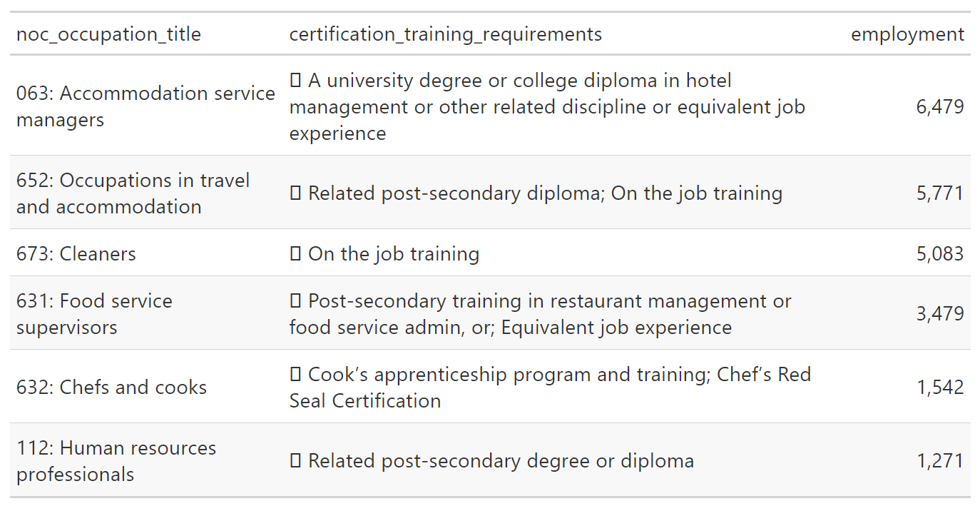
This table has four variables in three columns, each of which has at least one data cleaning challenge.
noc_occupation_title
This variable combines two values: the three-digit NOC code and the title of the occupation.
We will use the {tidyr} function separate_wider_delim() to split it into two variables. The function gives us the arguments to name the new columns that result from the separation and the character string that will be used to identify the separation point, in this case “:”. Don’t forget the space!
This function also has an argument cols_remove =. The default is set to TRUE, which removes the original column. Set to FALSE it retains the original column; we won’t use that here but it can be useful.
There are also separate_wider_() functions based on fixed-width positions and regular expressions.
noc_table_clean <- noc_table |>
  tidyr::separate_wider_delim(
    cols = noc_occupation_title,
    delim = ": ",
    names = c("noc", "occupation_title")
    )


gt(head(noc_table_clean))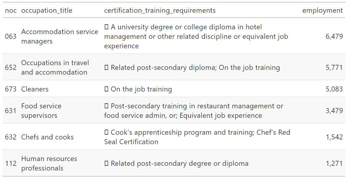
certification_training_requirements
This variable has a character that gets represented as a square at the beginning, and also a space between the square and the first letter.
Here we can use the {stringr} function str_remove_all(). (Remember that the str_remove() function removes only the first instance of the character.)
noc_table_clean <- noc_table_clean |>
mutate(
certification_training_requirements =
str_remove_all(certification_training_requirements, " ")
)
gt(head(noc_table_clean))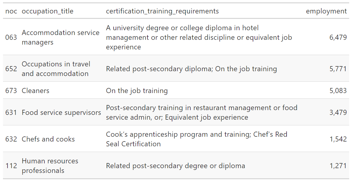
employment
This variable should be numbers but is a character type. This is because
there are commas used as the thousands separator
the smallest categories are represented with “-*” to indicate a table note.
In order to clean this, we require three steps:
remove commas
replace “-*” with NA
convert to numeric value
noc_table_clean <- noc_table_clean |>
  # remove commas
  mutate(
    employment =
      str_remove_all(employment, ",")
    ) |>
  # replace with NA
  mutate(
    employment =
      str_replace_all(employment, "-\\*", replacement = NA_character_)
    ) |>
  # convert to numeric
  mutate(
    employment =
      as.numeric(employment)
    )

gt(head(noc_table_clean))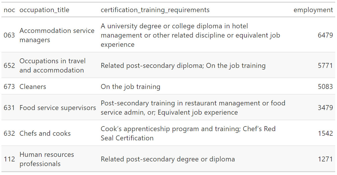
12.4 Creating conditional and calculated variables
We sometimes find ourselves in a situation where we want to recode our existing variables into other categories. An instance of this is when there are a handful of categories that make up the bulk of the total, and summarizing the smaller categories into an “all other” makes the table or plot easier to read. One example of this are the populations of the 13 Canadian provinces and territories: the four most populous provinces (Ontario, Quebec, British Columbia, and Alberta) account for roughly 85% of the country’s population…the other 15% of Canadians are spread across nine provinces and territories. We might want to show a table with only five rows, with the smallest nine provinces and territories grouped into a single row.
We can do this with a function in {dplyr}, case_when().
## # A tibble: 13 × 2
##    province_territory        population
##    <chr>                          <dbl>
##  1 Ontario                     13448494
##  2 Quebec                       8164361
##  3 British Columbia             4648055
##  4 Alberta                      4067175
##  5 Manitoba                     1278365
##  6 Saskatchewan                 1098352
##  7 Nova Scotia                   923598
##  8 New Brunswick                 747101
##  9 Newfoundland and Labrador     519716
## 10 Prince Edward Island          142907
## 11 Northwest Territories          41786
## 12 Nunavut                        35944
## 13 Yukon                          35874
In this first solution, we name the largest provinces separately:
canpop |>
  mutate(pt_grp = case_when(
    # evaluation ~ new value
    province_territory == "Ontario" ~ "Ontario",
    province_territory == "Quebec" ~ "Quebec",
    province_territory == "British Columbia" ~ "British Columbia",
    province_territory == "Alberta" ~ "Alberta",
    # all others get recoded as "other"
    TRUE ~ "other"
  ))
## # A tibble: 13 × 3
## province_territory population pt_grp
## <chr> <dbl> <chr>
## 1 Ontario 13448494 Ontario
## 2 Quebec 8164361 Quebec
## 3 British Columbia 4648055 British Columbia
## 4 Alberta 4067175 Alberta
## 5 Manitoba 1278365 other
## 6 Saskatchewan 1098352 other
## 7 Nova Scotia 923598 other
## 8 New Brunswick 747101 other
## 9 Newfoundland and Labrador 519716 other
## 10 Prince Edward Island 142907 other
## 11 Northwest Territories 41786 other
## 12 Nunavut 35944 other
## 13 Yukon 35874 otherBut that’s a lot of typing. A more streamlined approach is to put the name of our provinces in a list, and then recode our new variable with the value from the original variable province_territory:
canpop |>
  mutate(pt_grp = case_when(
    province_territory %in%
      c("Ontario", "Quebec", "British Columbia", "Alberta") ~
      province_territory,
    TRUE ~
      "other"
  ))
## # A tibble: 13 × 3
## province_territory population pt_grp
## <chr> <dbl> <chr>
## 1 Ontario 13448494 Ontario
## 2 Quebec 8164361 Quebec
## 3 British Columbia 4648055 British Columbia
## 4 Alberta 4067175 Alberta
## 5 Manitoba 1278365 other
## 6 Saskatchewan 1098352 other
## 7 Nova Scotia 923598 other
## 8 New Brunswick 747101 other
## 9 Newfoundland and Labrador 519716 other
## 10 Prince Edward Island 142907 other
## 11 Northwest Territories 41786 other
## 12 Nunavut 35944 other
## 13 Yukon 35874 otherWe could also use a comparison to create a population threshold, in this case four million:
canpop <- canpop |>
  mutate(pt_grp = case_when(
    population > 4000000 ~ province_territory,
    TRUE ~ "other"
  ))

canpop
## # A tibble: 13 × 3
## province_territory population pt_grp
## <chr> <dbl> <chr>
## 1 Ontario 13448494 Ontario
## 2 Quebec 8164361 Quebec
## 3 British Columbia 4648055 British Columbia
## 4 Alberta 4067175 Alberta
## 5 Manitoba 1278365 other
## 6 Saskatchewan 1098352 other
## 7 Nova Scotia 923598 other
## 8 New Brunswick 747101 other
## 9 Newfoundland and Labrador 519716 other
## 10 Prince Edward Island 142907 other
## 11 Northwest Territories 41786 other
## 12 Nunavut 35944 other
## 13 Yukon 35874 otherWhatever the approach we choose, that new variable can be used to group a table:
## # A tibble: 5 × 2
##   pt_grp             pt_pop
##   <chr>               <dbl>
## 1 Ontario          13448494
## 2 Quebec            8164361
## 3 other             4823643
## 4 British Columbia  4648055
## 5 Alberta           4067175
12.4.1 Classification systems
As we start to create new variables in our data, it is useful to be aware of various classification systems that already exist. That way, you can:
save yourself the challenge of coming up with your own classifications for your variables, and
ensure that your analysis can be compared to other results.
Of course, these classification systems are subject-matter specific.
As one example, in much social and business data, people’s ages are often grouped into 5-year “bins”, starting with ages 0–4, 5–9, 10–14, and so on. But not all age classification systems follow this; it will be driven by the specific context. The demographics of a workforce will not require a “0–4” category, while an analysis of school-age children might group them by the ages they attend junior, middle, and secondary school. As a consequence, many demographic tables will provide different data sets with the ages grouped in a variety of ways. (For an example, see (Statistics Canada 2007).)
And be aware that the elements with a classification system can change over time. One familiar example is that the geographical boundaries of cities and countries of the world have changed. City boundaries change, often with the more populous city expanding to absorb smaller communities within the larger legal entity. (The current City of Toronto is an amalgamation of what were six smaller municipalities.) Some regions have a rather turbulent history of changes in their boundaries, and some countries have been created only to disappear a few years later.
If you’re working in the area of social and economic research, the national and international statistics agencies provide robust and in-depth classification systems, much of which is explicitly designed to allow for international comparisons. These systems cover a wide range of economic and social statistics. Earlier in this chapter there was an example using the North American Industry Classification System (NAICS), used in Canada, the United States, and Mexico. Statistics Canada (2022). A similar classification system exists for Australia and New Zealand (Australian Bureau of Statistics 2006), and the European Union’s Eurostat office publishes a standard classification system for the products that are created through mining, manufacturing, and material recovery (EUROSTAT PRODCOM team 2022). For international statistics, you can start with the classification system maintained by the United Nations Statistics Division (United Nations Statistics Division 2020). In Chapter 6, we saw population statistics reported by the administrative geography of England and Wales.
Following these standardized categories in our own work is advantageous. It provides us with a validated structure, and should it be appropriate, gives us access to other data that can be incorporated into our own research.
Your subject area has established classifications; seek them out and use them. Ensuring that your data can be combined with and compared to other datasets will add value to your analysis, and make it easier for future researchers (including future you!) to work with your data. (White et al. 2013)
12.5 Indicator variables
To include a categorical variable in a regression, a natural approach is to construct an ‘indicator variable’ for each category. This allows a separate effect for each level of the category, without assuming any ordering or other structure on the categories. (Gelman et al. 2014, 366)
Indicator variables are also known as dummy variables (Suits 1957) and “one hot” encoding.
Examples of this approach abound. It can be a useful approach in forecasting methods; Hyndman and Athanasopoulos provide examples where public holidays and days of the week are set as dummy variables (R. J. Hyndman and Athanasopoulos 2021, sec. 7.4 “Some useful predictors”)
It is also a common approach in social data analysis, where categorical variables are used to code information. In the section on “Discrimination and collider bias” in (Cunningham 2021, 106–10), the data are represented in the following way 20:
## # A tibble: 6 × 5
##   female ability discrimination occupation   wage
##    <dbl>   <dbl>          <dbl>      <dbl>  <dbl>
## 1      0  -0.786              0     -0.555  0.162
## 2      1   2.81               1      4.93  11.6
## 3      1  -0.977              1     -4.23  -5.86
## 4      0   1.75               0      3.95  10.4
## 5      0   0.152              0      2.11   4.77
## 6      1  -0.561              1     -1.48  -3.41
In this data, the variable female is coded as numeric, so it can be used as part of the regression modelling.
More commonly, though, this variable will have been captured and saved in one called gender or sex, and often as a character string. The source data for the above table might have originally looked like this:
tb2 <- tb |>
  dplyr::rename(gender = female) |>
  mutate(gender = case_when(
    gender == 1 ~ "female",
    TRUE ~ "male"
))## # A tibble: 10 × 5
## gender ability discrimination occupation wage
## <chr> <dbl> <dbl> <dbl> <dbl>
## 1 male -0.786 0 -0.555 0.162
## 2 female 2.81 1 4.93 11.6
## 3 female -0.977 1 -4.23 -5.86
## 4 male 1.75 0 3.95 10.4
## 5 male 0.152 0 2.11 4.77
## 6 female -0.561 1 -1.48 -3.41
## 7 female 0.272 1 -1.56 -2.47
## 8 male 0.472 0 2.37 4.36
## 9 female 0.627 1 0.238 0.868
## 10 female 0.0128 1 -1.85 -2.5412.5.1 {fastDummies}
Because this type of data transformation is common, the package {fastDummies} (Kaplan and Schlegel 2020) has been created, containing the function dummy_cols() (or dummy_columns() if you prefer extra typing) that creates indicator variables.
If you are using the tidymodels pipeline, the {recipes} package (Kuhn and Wickham 2022) contains the
step_dummy()function, which accomplishes much the same result asfastDummies::dummy_cols(). The book Tidy modelling with R by Max Kuhn and Julia Silge (Kuhn and Silge 2022) is recommended; the creation of indicator variables is covered in Chapter 8, “Feature Engineering with recipes”.
## Rows: 10
## Columns: 7
## $ gender         <chr> "male", "female", "female", "male", "mal…
## $ ability        <dbl> -0.78648, 2.81050, -0.97717, 1.74628, 0.…
## $ discrimination <dbl> 0, 1, 1, 0, 0, 1, 1, 0, 1, 1
## $ occupation     <dbl> -0.5551, 4.9340, -4.2303, 3.9487, 2.1148…
## $ wage           <dbl> 0.1616, 11.6113, -5.8595, 10.4124, 4.774…
## $ gender_female  <int> 0, 1, 1, 0, 0, 1, 1, 0, 1, 1
## $ gender_male    <int> 1, 0, 0, 1, 1, 0, 0, 1, 0, 0
The variable gender has now been mutated into two additional variables, gender_female and gender_male. The names of the new variables are a concatenation of the original variable name and value, separated by an underscore.
Where the value of gender is “female”, the value of gender_female is assigned as “1”, and where gender is “male”, gender_female is “0”. This parallels what was in the original data. The opposite is true of gender_male; the rows where the value of gender is “male” gender_male has the value “1”.
Multicollinearity can occur in a multiple regression model where multiple indicator variables are included, since they are the inverse of one another. Accordingly, an important set of options in the dummy_cols() function revolve around removing all but one of the created variables. The argument remove_first_dummy = TRUE does just that; in this case, the gender_female() variable does not appear in the final result. This is because the new indicator variables are created in alphabetical order (“female” coming before “male”), and the first is dropped.
tb2_indicator <- tb2 |>
  fastDummies::dummy_cols(remove_first_dummy = TRUE)

glimpse(tb2_indicator, width = 65)
## Rows: 10
## Columns: 6
## $ gender <chr> "male", "female", "female", "male", "mal…
## $ ability <dbl> -0.78648, 2.81050, -0.97717, 1.74628, 0.…
## $ discrimination <dbl> 0, 1, 1, 0, 0, 1, 1, 0, 1, 1
## $ occupation <dbl> -0.5551, 4.9340, -4.2303, 3.9487, 2.1148…
## $ wage <dbl> 0.1616, 11.6113, -5.8595, 10.4124, 4.774…
## $ gender_male <int> 1, 0, 0, 1, 1, 0, 0, 1, 0, 0Note that the results of this argument can be controlled through the conversion of character variables to factors. To match the original dataframe, we would retain the variable gender_female.
# create new tb table with "gender" as factor
tb3 <- tb2 |>
  mutate(gender = as.factor(gender))

levels(tb3$gender)
## [1] "female" "male"Note that the default order is alphabetical, so “female” remains first. When the argument remove_first_dummy = TRUE is applied, we get the same result as before.
## Rows: 10
## Columns: 6
## $ gender         <fct> male, female, female, male, male, female…
## $ ability        <dbl> -0.78648, 2.81050, -0.97717, 1.74628, 0.…
## $ discrimination <dbl> 0, 1, 1, 0, 0, 1, 1, 0, 1, 1
## $ occupation     <dbl> -0.5551, 4.9340, -4.2303, 3.9487, 2.1148…
## $ wage           <dbl> 0.1616, 11.6113, -5.8595, 10.4124, 4.774…
## $ gender_male    <int> 1, 0, 0, 1, 1, 0, 0, 1, 0, 0
By using the fct_relevel() function from the {forcats}(Wickham 2021a) package, we can assign an arbitrary order.
## [1] "male" "female"Rerunning the same code, the gender_male variable is dropped.
## Rows: 10
## Columns: 6
## $ gender         <fct> male, female, female, male, male, female…
## $ ability        <dbl> -0.78648, 2.81050, -0.97717, 1.74628, 0.…
## $ discrimination <dbl> 0, 1, 1, 0, 0, 1, 1, 0, 1, 1
## $ occupation     <dbl> -0.5551, 4.9340, -4.2303, 3.9487, 2.1148…
## $ wage           <dbl> 0.1616, 11.6113, -5.8595, 10.4124, 4.774…
## $ gender_female  <int> 0, 1, 1, 0, 0, 1, 1, 0, 1, 1
There is also an option in fastDummies::dummy_cols() to remove_most_frequent_dummy = TRUE. In our discrimination data, there are more observations coded as “female”, so the variable gender_female is not included.
tb2_frequent <- tb2 |>
  fastDummies::dummy_cols(remove_most_frequent_dummy = TRUE)

glimpse(tb2_frequent, width = 65)
## Rows: 10
## Columns: 6
## $ gender <chr> "male", "female", "female", "male", "mal…
## $ ability <dbl> -0.78648, 2.81050, -0.97717, 1.74628, 0.…
## $ discrimination <dbl> 0, 1, 1, 0, 0, 1, 1, 0, 1, 1
## $ occupation <dbl> -0.5551, 4.9340, -4.2303, 3.9487, 2.1148…
## $ wage <dbl> 0.1616, 11.6113, -5.8595, 10.4124, 4.774…
## $ gender_male <int> 1, 0, 0, 1, 1, 0, 0, 1, 0, 0Another argument in the function is remove_selected_columns. The default value is FALSE, but if the argument is set to TRUE, the source column is excluded from the output.
tb2_select <- tb2 |>
  fastDummies::dummy_cols(remove_selected_columns = TRUE)

glimpse(tb2_select, width = 65)
## Rows: 10
## Columns: 6
## $ ability <dbl> -0.78648, 2.81050, -0.97717, 1.74628, 0.…
## $ discrimination <dbl> 0, 1, 1, 0, 0, 1, 1, 0, 1, 1
## $ occupation <dbl> -0.5551, 4.9340, -4.2303, 3.9487, 2.1148…
## $ wage <dbl> 0.1616, 11.6113, -5.8595, 10.4124, 4.774…
## $ gender_female <int> 0, 1, 1, 0, 0, 1, 1, 0, 1, 1
## $ gender_male <int> 1, 0, 0, 1, 1, 0, 0, 1, 0, 0Some important things to note about dummy_cols()
the function will create as many indicator variables as there are values in the character or factor variable
the function will create indicator variables for all of the character and factor variables in the data, unless otherwise specified.
Let’s look at how dummy_cols() behaves with two of the variables in {palmerpenguins}:
library(palmerpenguins)

set.seed(1729) # Ramanujan's taxicab number: 1^3 + 12^3 = 9^3 + 10^3

penguin_subset <- penguins |>
  slice_sample(n = 6) |>
  dplyr::select(species, island) |>
arrange(species)## # A tibble: 6 × 2
## species island
## <fct> <fct>
## 1 Adelie Biscoe
## 2 Adelie Torgersen
## 3 Chinstrap Dream
## 4 Gentoo Biscoe
## 5 Gentoo Biscoe
## 6 Gentoo Biscoepenguin_subset_1 <- penguin_subset |>
fastDummies::dummy_cols()
glimpse(penguin_subset_1, width = 65)## Rows: 6
## Columns: 8
## $ species <fct> Adelie, Adelie, Chinstrap, Gentoo, Ge…
## $ island <fct> Biscoe, Torgersen, Dream, Biscoe, Bis…
## $ species_Adelie <int> 1, 1, 0, 0, 0, 0
## $ species_Chinstrap <int> 0, 0, 1, 0, 0, 0
## $ species_Gentoo <int> 0, 0, 0, 1, 1, 1
## $ island_Biscoe <int> 1, 0, 0, 1, 1, 1
## $ island_Dream <int> 0, 0, 1, 0, 0, 0
## $ island_Torgersen <int> 0, 1, 0, 0, 0, 0First, you will notice that we started with two factor variables, species and island; we now have indicator variables for both.
And because there are three species of penguins and three islands, we have three indicator variables for both of the original variables.
In the instance where we have multiple character or factor variables in our source data, we can control which variables get the dummy_cols() treatment with the option, select_columns. In the example below, the result provides us with an indicator variable for species but not island.
In addition, rather than dropping the first created variable, we can specify that the most frequently occurring value be removed with the argument remove_most_frequent_dummy = TRUE. Because there are more Gentoo penguins in our sample of the data, the indicator variable species_Gentoo is not created.
penguin_subset_2 <- penguin_subset |>
  fastDummies::dummy_cols(
    select_columns = "species",
    remove_most_frequent_dummy = TRUE)

glimpse(penguin_subset_2, width = 65)
## Rows: 6
## Columns: 4
## $ species <fct> Adelie, Adelie, Chinstrap, Gentoo, Ge…
## $ island <fct> Biscoe, Torgersen, Dream, Biscoe, Bis…
## $ species_Adelie <int> 1, 1, 0, 0, 0, 0
## $ species_Chinstrap <int> 0, 0, 1, 0, 0, 012.6 Missing values
Frequently, our data will have missing values. Some of this will be gaps in the data, and in other cases it will be due to the structure of the source data file.
There are a variety of solutions to dealing with gaps in data values (sometimes called “missingness”), from listwise deletion (removing all rows with missing values) to complex algorithms that apply methods to impute the best estimate of the missing value. There is in-depth literature on this topic (see (Little 2020), (Gelman et al. 2014, chap. 18), and (Gelman and Hill 2007, chap. 25)); what is presented here are some solutions to common and relatively simple problems.
12.6.1 Missing as formatting
A common spreadsheet formatting practice that makes the tables human-readable but less analysis-ready is to have a sub-section heading, often in a separate column. In the example Excel file that we will use for this, the sheet “Report” contains data on tuition fees paid by international students in British Columbia, arranged in a wide format. The name of the individual institution is in the second column (in Excel nomenclature, “B”), and the region (“Economic Development Region”) is in the first column. However, the name of the region only appears in the row above the institutions in that region. This makes for a nicely formatted table, but isn’t very helpful if we are trying to calculate average tuition fees by region.21
Our first step is to read in the data. Note that the code uses the Excel naming convention to define the rectangular range to be read and omits the title rows at the top and the notes at the bottom of the sheet.
tuition_data <-
  readxl::read_excel(dpjr::dpjr_data("intl_tuition_fees_bc.xlsx"),
                     sheet = "Report",
                     range = "A5:L36")

head(tuition_data)
## # A tibble: 6 × 12
## Economic Development…¹ Institution `AY 2012/13` `AY 2013/14` `AY 2014/15`
## <chr> <chr> <dbl> <dbl> <dbl>
## 1 Mainland/Southwest <NA> NA NA NA
## 2 <NA> British Co… 17611. 17963. 18323.
## 3 <NA> Capilano U… 15000 15750 16170
## 4 <NA> Douglas Co… 14400 15000 15300
## 5 <NA> Emily Carr… 15000. 15600 16224.
## 6 <NA> Justice In… 13592. 13864. 14141.
## # ℹ abbreviated name: ¹`Economic Development Region`
## # ℹ 7 more variables: `AY 2015/16` <dbl>, `AY 2016/17` <dbl>,
## # `AY 2017/18` <dbl>, `AY 2018/19` <dbl>, `AY 2019/20` <dbl>,
## # `AY 2020/21` <dbl>, `AY 2021/22` <dbl>The contents of the file have been read correctly, but there are many “NA” values in the Economic Development Region variable. This is due to the manner in which the data was structured in the source Excel file.
The fill() function, in the {tidyr} package (Wickham 2021b), provides the solution to this. The function replaces a missing value with either the previous or the next value in a variable. In the example here, it will replace all of the “NA” values with the region name above, stopping when it comes to the next non-NA record.
tuition_data_filled <- tuition_data |>
  fill("Economic Development Region")

head(tuition_data_filled)
## # A tibble: 6 × 12
## Economic Development…¹ Institution `AY 2012/13` `AY 2013/14` `AY 2014/15`
## <chr> <chr> <dbl> <dbl> <dbl>
## 1 Mainland/Southwest <NA> NA NA NA
## 2 Mainland/Southwest British Co… 17611. 17963. 18323.
## 3 Mainland/Southwest Capilano U… 15000 15750 16170
## 4 Mainland/Southwest Douglas Co… 14400 15000 15300
## 5 Mainland/Southwest Emily Carr… 15000. 15600 16224.
## 6 Mainland/Southwest Justice In… 13592. 13864. 14141.
## # ℹ abbreviated name: ¹`Economic Development Region`
## # ℹ 7 more variables: `AY 2015/16` <dbl>, `AY 2016/17` <dbl>,
## # `AY 2017/18` <dbl>, `AY 2018/19` <dbl>, `AY 2019/20` <dbl>,
## # `AY 2020/21` <dbl>, `AY 2021/22` <dbl>The next step is to use the {tidyr} function drop_na() to omit any row that contains an NA value. In this case, we want to drop what were the header rows that contained just the region name in the first column and no values in the other columns.
These two solutions yield the same result:
## # A tibble: 25 × 12
##    `Economic Development Region` Institution      `AY 2012/13` `AY 2013/14`
##    <chr>                         <chr>                   <dbl>        <dbl>
##  1 Mainland/Southwest            British Columbi…       17611.       17963.
##  2 Mainland/Southwest            Capilano Univer…       15000        15750
##  3 Mainland/Southwest            Douglas College        14400        15000
##  4 Mainland/Southwest            Emily Carr Univ…       15000.       15600
##  5 Mainland/Southwest            Justice Institu…       13592.       13864.
##  6 Mainland/Southwest            Kwantlen Polyte…       15000        15750
##  7 Mainland/Southwest            Langara College        16500        16950
##  8 Mainland/Southwest            Simon Fraser Un…       16236        17862
##  9 Mainland/Southwest            University of B…       22622.       23300.
## 10 Mainland/Southwest            University of t…       12720        13350
## # ℹ 15 more rows
## # ℹ 8 more variables: `AY 2014/15` <dbl>, `AY 2015/16` <dbl>,
## #   `AY 2016/17` <dbl>, `AY 2017/18` <dbl>, `AY 2018/19` <dbl>,
## #   `AY 2019/20` <dbl>, `AY 2020/21` <dbl>, `AY 2021/22` <dbl>
It’s worth noting that the drop_na() function provides an argument where we can specify columns. This gives us the flexibility to drop some rows where there is an “NA” in a specific variable, while keeping other rows that have a value in that variable but not in other variables.
12.6.2 Missing numeric values
“Missing data are unobserved values that would be meaningful for analysis if observed; in other words, a missing value hides a meaningful value.” (Little 2020)
The functions used above for filling missing text values can also be used for missing numeric values. But when dealing with the replacement of numeric values, we need to be mindful that the values we use will be incorporated into models and analysis; we need to be clear that the filled values are estimates, including sufficient documentation in our methodology section.
Furthermore, there is a great deal of literature on the topic of imputation of missing values. As researchers, we need to be aware of why the values are missing; are we dealing with values that are missing “at completely random,” “at random,” or “not at random?” Delving into the literature, you’ll discover that these terms are precisely defined, and the solutions we adopt to deal with missingness will depend on the reason (or reasons) why the data are missing. (Little 2020)
For the examples presented here, we will assume that you have already given significant thought to these methodological questions. As we discussed earlier in this chapter, how we clean data is influenced by our research questions. As well, we need to consider our cleaning strategy in light of why the raw data are the way they are.
With that preamble, let’s move to working with some real data. In this example, the data series is the number of salaried employees in the Accommodation services industry in British Columbia, Canada, for the years 2001 through 2020. The data are collected and published by Statistics Canada, and for some years the data are judged to be “too unreliable to be published.” This leaves some gaps in our data.
## # A tibble: 6 × 4
##   label    ref_year REF_DATE   VALUE
##   <chr>       <dbl> <chr>      <dbl>
## 1 Salaried     2001 2001-01-01  4458
## 2 Salaried     2002 2002-01-01  4392
## 3 Salaried     2003 2003-01-01  4124
## 4 Salaried     2004 2004-01-01  4828
## 5 Salaried     2005 2005-01-01  4069
## 6 Salaried     2006 2006-01-01  5048
We will employ Exploratory Data Analysis, and plot the data:
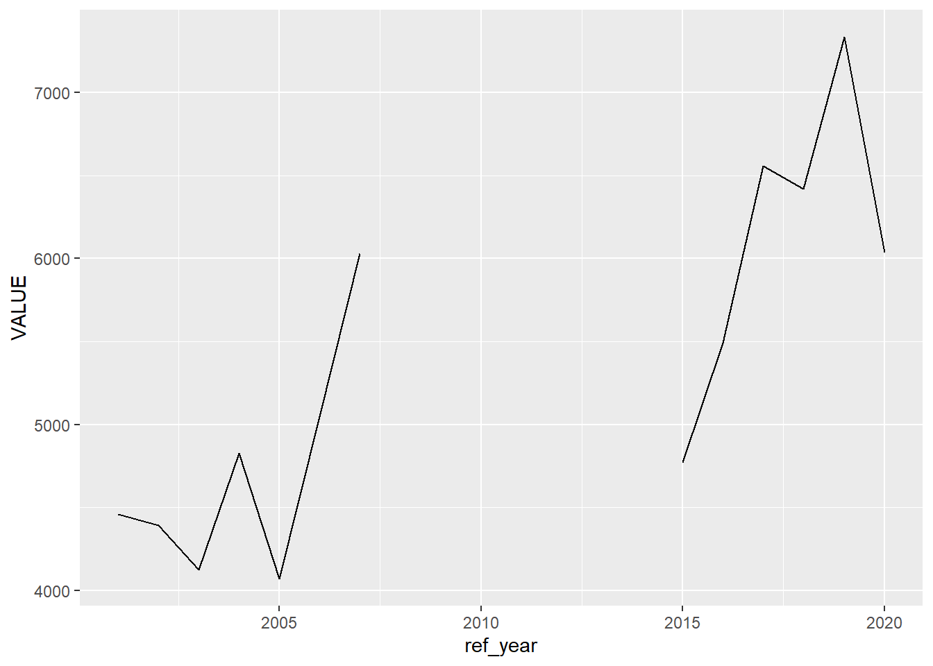
Our first approach will be to simply drop those years that are missing a value. This might help with some calculations (for example, putting a na.rm = TRUE argument in a mean() function is doing just that), but it will create a misleading plot—there will be the same distance between the 2009 and 2015 points as there is between 2015 and 2016.
## # A tibble: 5 × 4
## label ref_year REF_DATE VALUE
## <chr> <dbl> <chr> <dbl>
## 1 Salaried 2001 2001-01-01 4458
## 2 Salaried 2002 2002-01-01 4392
## 3 Salaried 2003 2003-01-01 4124
## 4 Salaried 2004 2004-01-01 4828
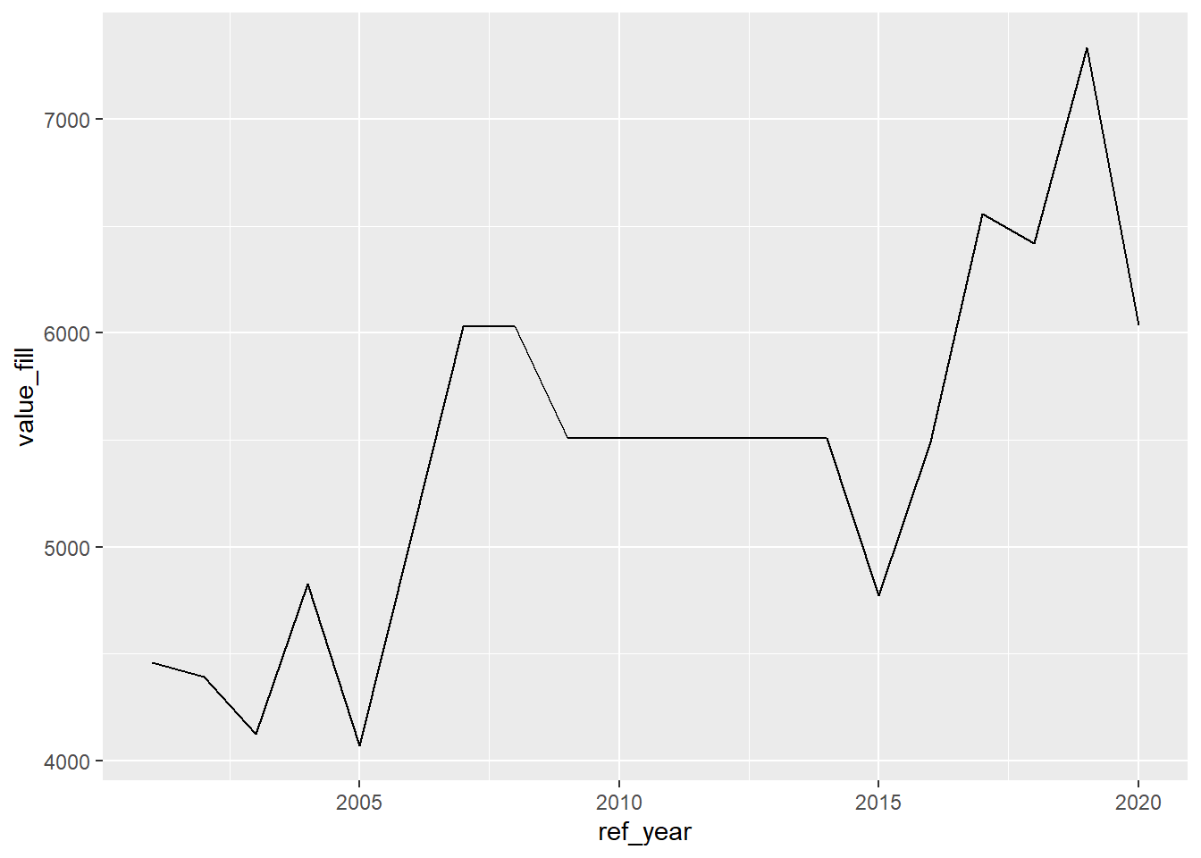
## 5 Salaried 2005 2005-01-01 4069Alternatively, we can fill the series with the previous valid entry.
Similar to what we saw above with text, the same fill() function can be applied to numeric variables. We will first create a variable new_value that will house the same value as our existing variable; the fill() function will be applied to new_value.
# fill down
naics721_sal_new <- naics721_sal |>
  mutate(value_fill = VALUE) |>
  tidyr::fill(value_fill)  # default direction is down

naics721_sal_new
## # A tibble: 20 × 5
## label ref_year REF_DATE VALUE value_fill
## <chr> <dbl> <chr> <dbl> <dbl>
## 1 Salaried 2001 2001-01-01 4458 4458
## 2 Salaried 2002 2002-01-01 4392 4392
## 3 Salaried 2003 2003-01-01 4124 4124
## 4 Salaried 2004 2004-01-01 4828 4828
## 5 Salaried 2005 2005-01-01 4069 4069
## 6 Salaried 2006 2006-01-01 5048 5048
## 7 Salaried 2007 2007-01-01 6029 6029
## 8 Salaried 2008 2008-01-01 NA 6029
## 9 Salaried 2009 2009-01-01 5510 5510
## 10 Salaried 2010 2010-01-01 NA 5510
## 11 Salaried 2011 2011-01-01 NA 5510
## 12 Salaried 2012 2012-01-01 NA 5510
## 13 Salaried 2013 2013-01-01 NA 5510
## 14 Salaried 2014 2014-01-01 NA 5510
## 15 Salaried 2015 2015-01-01 4772 4772
## 16 Salaried 2016 2016-01-01 5492 5492
## 17 Salaried 2017 2017-01-01 6557 6557
## 18 Salaried 2018 2018-01-01 6420 6420
## 19 Salaried 2019 2019-01-01 7334 7334
## 20 Salaried 2020 2020-01-01 6036 6036Now when we plot the data, the missing points are shown:
There are a few different options to determine which way to fill; the default is .direction = "down".
12.6.3 Time series imputation
You may already have realized that the values we filled above are drawn from a time series. Economists, biologists, and many other researchers who work with time series data have built up a large arsenal of tools to work with time series data, including robust methodologies for dealing with missing values.
For R users, the package {forecast} has time series-oriented imputation fill functions. (R. Hyndman et al. 2023; R. J. Hyndman and Khandakar 2008)
The na.interp() function from {forecast} gives us a much better way to fill the missing values in our time series than simply extending known values. This function, by default, uses a linear interpolation to calculate values between two non-missing values. Here’s a simple example:
## [1] 1 NA 3The series from 1 to 3 has an NA value in the middle. The na.interp() function fills in the missing value.
## Time Series:
## Start = 1
## End = 3
## Frequency = 1
## [1] 1 2 3
For longer series, a similar process occurs:
## [1] 1 NA NA 3## Time Series:
## Start = 1
## End = 4
## Frequency = 1
## [1] 1.000 1.667 2.333 3.000You will notice that the function has calculated replacement values that give us a linear series.
For our count of salaried employees, here’s what we get when we create a new value, value_new, with this function:
## # A tibble: 20 × 5
##    label    ref_year REF_DATE   VALUE value_interp
##    <chr>       <dbl> <chr>      <dbl>        <dbl>
##  1 Salaried     2001 2001-01-01  4458        4458
##  2 Salaried     2002 2002-01-01  4392        4392
##  3 Salaried     2003 2003-01-01  4124        4124
##  4 Salaried     2004 2004-01-01  4828        4828
##  5 Salaried     2005 2005-01-01  4069        4069
##  6 Salaried     2006 2006-01-01  5048        5048
##  7 Salaried     2007 2007-01-01  6029        6029
##  8 Salaried     2008 2008-01-01    NA        5770.
##  9 Salaried     2009 2009-01-01  5510        5510
## 10 Salaried     2010 2010-01-01    NA        5387
## 11 Salaried     2011 2011-01-01    NA        5264
## 12 Salaried     2012 2012-01-01    NA        5141
## 13 Salaried     2013 2013-01-01    NA        5018
## 14 Salaried     2014 2014-01-01    NA        4895
## 15 Salaried     2015 2015-01-01  4772        4772
## 16 Salaried     2016 2016-01-01  5492        5492
## 17 Salaried     2017 2017-01-01  6557        6557
## 18 Salaried     2018 2018-01-01  6420        6420
## 19 Salaried     2019 2019-01-01  7334        7334
## 20 Salaried     2020 2020-01-01  6036        6036
Plotting the data with the interpolated values, there are no gaps.
## Don't know how to automatically pick scale for object of type <ts>.
## Defaulting to continuous.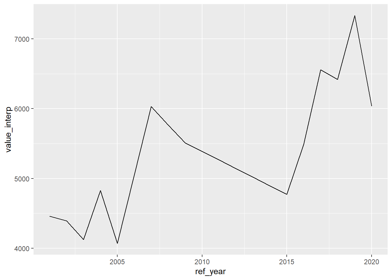
The na.interp() function also has the capacity to create non-linear models.
Other examples of time series missing value imputation functions can be found in the {imputeTS} package (Moritz and Bartz-Beielstein 2017), which offers multiple imputation algorithms and plotting functions. A fantastic resource for using R for time series analysis, including a section on imputation of missing values, is (R. J. Hyndman and Athanasopoulos 2021).
12.7 Creating labelled factors from numeric variables
In Chapter 7 we imported statistical software packages such as SPSS, SAS, or Stata and saw the benefits, in certain circumstances, of having labelled variables. These are categorical variables, where there are a limited number of categories.
In some cases, there might be one or more values assigned to categories we might want to designate as “missing”—a common example can be found in surveys, where respondents are given the option of answering “don’t know” and “not applicable.” While these responses might be interesting in and of themselves, in some contexts we will want to assign them as missing.
In other cases, numeric values are used to store the categorical responses.
The Joint Canada/United States Survey of Health (JCUSH) file we saw in Chapter 5 importing fixed width files gives us a good example of where categories are stored as numerical variables. For example, the variable SPJ1_TYP is either a “1” for responses from the Canadian sample and a “2” for the sample from the United States.
We will use this file to create labelled factors from the numeric values in the variables we imported. Here’s the code we used previously to read the file:
jcush <- readr::read_fwf(dpjr::dpjr_data("JCUSH.txt"),
         fwf_cols(
           SAMPLEID = c(1, 12),
           SPJ1_TYP = c(13, 13),
           GHJ1DHDI = c(32, 32),
           SDJ1GHED = c(502, 502)
           ),
         col_types = list(
           SAMPLEID = col_character()
         ))

head(jcush)
## # A tibble: 6 × 4
## SAMPLEID SPJ1_TYP GHJ1DHDI SDJ1GHED
## <chr> <dbl> <dbl> <dbl>
## 1 100003330835 1 3 4
## 2 100004903392 1 3 2
## 3 100010137168 1 2 1
## 4 100010225523 1 3 3
## 5 100011623697 1 2 2
## 6 100013652729 1 4 3The values for these variables are as follows:
| Name | Variable | Code | Value |
|---|---|---|---|
| SAMPLEID | Household identifier | unique number | |
| SPJ1_TYP | Sample type [country] | 1 | Canada |
| 2 | United States | ||
| GHJ1DHDI | Health Description Index | 0 | Poor |
| 1 | Fair | ||
| 2 | Good | ||
| 3 | Very Good | ||
| 4 | Excellent | ||
| 9 | Not Stated | ||
| SDJ1GHED | Highest level of post-secondary education attained | 1 | Less than high school |
| 2 | High school degree or equivalent (GED) | ||
| 3 | Trades Cert, Voc. Sch./Comm.Col./CEGEP | ||
| 4 | Univ or Coll. Cert. incl. below Bach. | ||
| 9 | Not Stated |
The variable GHJ1DHDI has the respondent’s self-assessment of their overall health. Here’s a summary table of the responses:
## # A tibble: 6 × 2
##   GHJ1DHDI     n
##      <dbl> <int>
## 1        0   391
## 2        1   891
## 3        2  2398
## 4        3  2914
## 5        4  2082
## 6        9    12
But it would be much more helpful and efficient if we attach the value labels to the dataframe.
One strategy is to create a new factor variable, that uses the value description instead of the numeric representation. For this, we will use the fct_recode() function from the {forcats} package(Wickham 2021a).
library(forcats)

jcush_forcats <- jcush |>
  # 1st mutate a new factor variable with the original values
  mutate(health_desc_fct = as.factor(GHJ1DHDI)) |>
  # 2nd recode the values
  mutate(
    health_desc_fct = fct_recode(
      health_desc_fct,
      "Poor" = "0",
      "Fair" = "1",
      "Good" = "2",
      "Very Good" = "3",
      "Excellent" = "4",
      NULL = "9"
    )
  )
The levels() function allows us to inspect the labels. Note that because we specified the original value of “9” as NULL, it does not appear in the list.
## [1] "Poor" "Fair" "Good" "Very Good" "Excellent"When we tally the results by our new variable, the GHJ1DHDI records with the value 9 are shown as “NA”.
## # A tibble: 6 × 3
## # Groups:   GHJ1DHDI [6]
##   GHJ1DHDI health_desc_fct     n
##      <dbl> <fct>           <int>
## 1        0 Poor              391
## 2        1 Fair              891
## 3        2 Good             2398
## 4        3 Very Good        2914
## 5        4 Excellent        2082
## 6        9 <NA>               12
Another option is provided in the {haven} package (Wickham and Miller 2021).
library(haven)

jcush_haven <- jcush |>
  mutate(health_desc_lab = labelled(
    GHJ1DHDI,
    c(
      "Poor" = 0,
      "Fair" = 1,
      "Good" = 2,
      "Very Good" = 3,
      "Excellent" = 4,
      "Not Stated" = 9
    )
  ))
Note that our new variable is a “S3: haven_labelled” class, and the ls.str() function shows it as “dbl+lbl”:
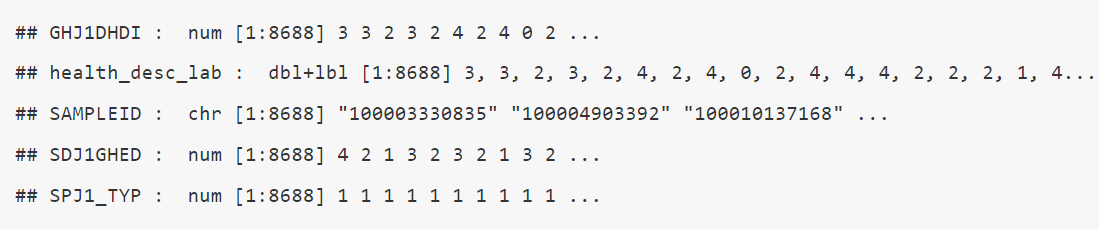
The levels() function can be used to inspect the result of this mutate.
## <labelled<double>[6]>
## [1] 3 3 2 3 2 4
##
## Labels:
##  value      label
##      0       Poor
##      1       Fair
##      2       Good
##      3  Very Good
##      4  Excellent
##      9 Not Stated
A third option is to use the functions within the {labelled} package (Larmarange 2022).
jcush_labelled <- jcush |>
  mutate(health_desc_lab = labelled(
    GHJ1DHDI,
    c(
      "Poor" = 0,
      "Fair" = 1,
      "Good" = 2,
      "Very Good" = 3,
      "Excellent" = 4,
      "Not Stated" = 9
    )
  ))
To view a single variable, use:
## <labelled<double>[6]>
## [1] 3 3 2 3 2 4
##
## Labels:
##  value      label
##      0       Poor
##      1       Fair
##      2       Good
##      3  Very Good
##      4  Excellent
##      9 Not Stated
This package also allows for a descriptive name of the variable to be appended with the var_lab() function.
References
The full list of unicode characters can be found at the Wikipedia webpage (Wikipedia contributors 2022a).↩︎
Note: the data in this table is different from what appears in Causal Inference: The Mixtape, since the values in the data in that source are randomly generated.↩︎
The creators of the file have provided us with a tidy sheet named “Data” and deserve kudos for sharing the data in a variety of layouts. But please be aware that this approach is the exception, not the rule.↩︎