Chapter 6 Importing data: Excel

In this chapter:

Importing data from Excel spreadsheets
Extracting data that is encoded as Excel formatting

6.1 Introduction

Spreadsheets and similar data tables are perhaps the most common way that data is made available. Because they originated as an electronic version of accounting worksheets, they have a tabular structure that works for other situations when data collection, storage, analysis, and sharing (i.e. publishing) are required. Spreadsheet software of one form or another is often standard when you buy a new computer, and Microsoft Excel is the most common of all. Google also makes available a web-based spreadsheet tool, Google Sheets that works in much the same way.

While the data in a spreadsheet often gets stored in a manner similar to a plain-text file such as the CSV files we worked with in the previous chapter, Excel is designed to deliver far more functionality.

Broman and Woo (Broman and Woo 2017) provide a how-to for good data storage practice in a spreadsheet, but you are much more likely to find yourself working with a spreadsheet that doesn’t achieve that standard. Paul Murrell titled his article “Data Intended for Human Consumption, Not Machine Consumption” (Murrell 2013) for a reason: all too often, a spreadsheet is used to make data easy for you and me to read, but this makes it harder for us to get it into a structure where our software program can do further analysis.

Spreadsheets like Excel also have a dark side (at least when it comes to data storage)—the values you see are not necessarily what’s in the cell. For example, a cell might be the result of an arithmetic function that brings one or more values from elsewhere in the sheet (or in some cases, from another sheet, or anther sheet in another file). Some users will colour-code cells, but with no index to tell you what each colour means. (Bryan 2016b) (For an alternative vision, see “Sanesheets” (Bryan 2016a).)

The “format as data” and “formatting as information” approaches of storing information can make it hard for us to undertake our analysis. Excel files can also contain a wide variety of data format types. For example, when using Excel you will find that leading or trailing whitespace makes a number turn into a character, even if the cell is given an Excel number format.

The {readxl} package (Wickham and Bryan 2019) is designed to solve many of the challenges of reading Excel files. To access the functions in {readxl}, we use the library() function to load the package into our active project:

library(readxl)

{readxl} tries to figure out what’s going on with each variable, but like {readr} it allows you to override some of those automated decisions if it returns something different than what the analysis calls for. The {readxl} arguments we will use include the following:

argument	purpose
`sheet = ""`	a character string with the name of the sheet in the Excel workbook to be read
`range = ""`	define the rectangle to be read; see the examples below for syntax options
`skip = 0`	specify how many rows to skip; the default is 0
`n_max = Inf`	the maximum number of records to read; the default is `Inf` for infinity, interpreted as the last row of the file

For this example, we will use some mock data that is the type a data analyst might encounter when undertaking analysis of human resource data to support business decision-making. The file “cr25_human_resources.xlsx” is in the folder “cr25”.

Because Excel files can contain multiple sheets, we need to specify which one we want to read. The {readxl} function excel_sheets() lists them for us:

excel_sheets(dpjr::dpjr_data("cr25/cr25_human_resources.xlsx"))

## [1] "readme"            "df_HR_main"       
## [3] "df_HR_transaction" "df_HR_train"

The one we want for our example is “df_HR_main”, which contains the employee ID, name, birth date, and gender for each of the 999 staff.

In our read_excel() function we can specify either the name of the sheet or the number based on its position in the Excel file. While the default is to read the first sheet, it’s often good practice to be specific, as Excel users are prone to re-arranging the order of the sheets (including adding new sheets). And because they seem (slightly) less likely to rename sheets, we have another reason to use the name rather than the number.

df_HR_main <- 
  read_excel(
    path = dpjr::dpjr_data("cr25/cr25_human_resources.xlsx"),
    sheet = "df_HR_main"
    )

## New names:
## • `` -> `...2`
## • `` -> `...3`
## • `` -> `...4`
## • `` -> `...5`
## • `` -> `...6`
## • `` -> `...7`

head(df_HR_main)

## # A tibble: 6 × 7
##   df_HR_main        ...2  ...3  ...4  ...5  ...6  ...7 
##   <chr>             <chr> <chr> <chr> <chr> <lgl> <chr>
## 1 The main databas… <NA>  <NA>  <NA>  <NA>  NA    <NA> 
## 2 <NA>              <NA>  <NA>  <NA>  <NA>  NA    <NA> 
## 3 <NA>              <NA>  <NA>  <NA>  <NA>  NA    <NA> 
## 4 <NA>              emp_… date… name  gend… NA    NOTE:
## 5 <NA>              ID001 29733 Avri… Fema… NA    date…
## 6 <NA>              ID002 26931 Katy… Fema… NA    <NA>

This sheet possesses a structure we commonly see in Excel files: in addition to the data of interest, the creators of the file have helpfully added a title for the sheet. They might also put a note in the “margins” of the data (often to the right or below the data), and add formatting to make it more visually appealing to human readers (beware empty or hidden columns and rows!).

While this is often useful information, its presence means that we need to trim rows and columns to get our dataframe in a useful structure for our analysis.

The read_excel() function provides a number of different ways for us to define the range that will be read. One that works well in the function, and aligns with how many Excel users think about their spreadsheets, defines the upper left and the lower right corners of the data using Excel’s column-row alpa-numeric nomenclature. For this file, that will exclude the top rows, the empty columns to the left and right of the data, as well as the additional note to the right. The corners are cells B5 and E1004. How did I know that?

Important note: there is no shame in opening the file in Excel to make a visual scan of the file, looking for anomalous values and to note the corners of the data rectangle.

df_HR_main <- 
  read_excel(
    path = dpjr::dpjr_data("cr25/cr25_human_resources.xlsx"),
    sheet = "df_HR_main",
    range = "B5:E1004"
    )

head(df_HR_main)

## # A tibble: 6 × 4
##   emp_id date_of_birth       name               gender
##   <chr>  <dttm>              <chr>              <chr> 
## 1 ID001  1981-05-27 00:00:00 Avril Lavigne      Female
## 2 ID002  1973-09-24 00:00:00 Katy Perry         Female
## 3 ID003  1966-11-29 00:00:00 Chester Bennington Male  
## 4 ID004  1982-09-17 00:00:00 Chris Cornell      Male  
## 5 ID005  1976-07-17 00:00:00 Bryan Adams        Male  
## 6 ID006  1965-07-03 00:00:00 Courtney Love      Female

The range = argument also gives us the option to use Excel’s row number-column number specification, which would change the above range = "B5:E1004" to range = "R5C2:R1004C5" (“B” refers to the second column, and “E” to the fifth).

df_HR_main <- 
  read_excel(
    path = dpjr::dpjr_data("cr25/cr25_human_resources.xlsx"),
    sheet = "df_HR_main",
    range = "R5C2:R1004C5"
    )

There are a variety of other approaches to defining the data rectangle in a read_excel() function, which might be more appropriate in a different context. For example, if the sheet is continually having new rows added at the bottom, using the range = anchored("B5", dim =c(NA, 4)) specification might be prefered. This will start at cell B5, then read as many rows as there are data (the “NA” inside the c() function and four columns.⁷

df_HR_main <- 
  read_excel(
    path = dpjr::dpjr_data("cr25/cr25_human_resources.xlsx"),
    sheet = "df_HR_main",
    range = anchored("B5", dim =c(NA, 4))
    )

head(df_HR_main)

## # A tibble: 6 × 4
##   emp_id date_of_birth       name               gender
##   <chr>  <dttm>              <chr>              <chr> 
## 1 ID001  1981-05-27 00:00:00 Avril Lavigne      Female
## 2 ID002  1973-09-24 00:00:00 Katy Perry         Female
## 3 ID003  1966-11-29 00:00:00 Chester Bennington Male  
## 4 ID004  1982-09-17 00:00:00 Chris Cornell      Male  
## 5 ID005  1976-07-17 00:00:00 Bryan Adams        Male  
## 6 ID006  1965-07-03 00:00:00 Courtney Love      Female

Another splendid feature of read_excel() is that it returns a date type (S3: POSIXct) for variables that it interprets as dates.

6.2 Extended example

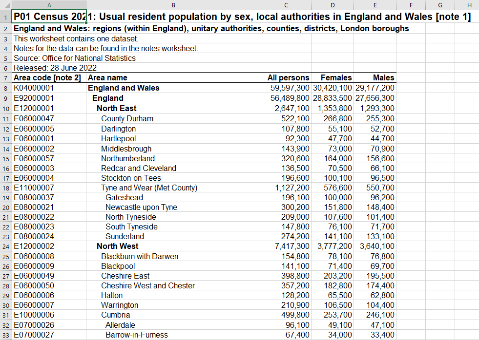
Very often, Excel files are far more complicated than the case above. In the following example, we will read the contents of one sheet in an Excel file published by the UK Office of National Statistics, drawn from the 2021 Census of England and Wales. The file “census2021firstresultsenglandwales1.xlsx” has the population by local authorities (regions), and includes sheets with notes about the data, and data tables containing the population by sex and five-year age groups, along with population density and number of households.

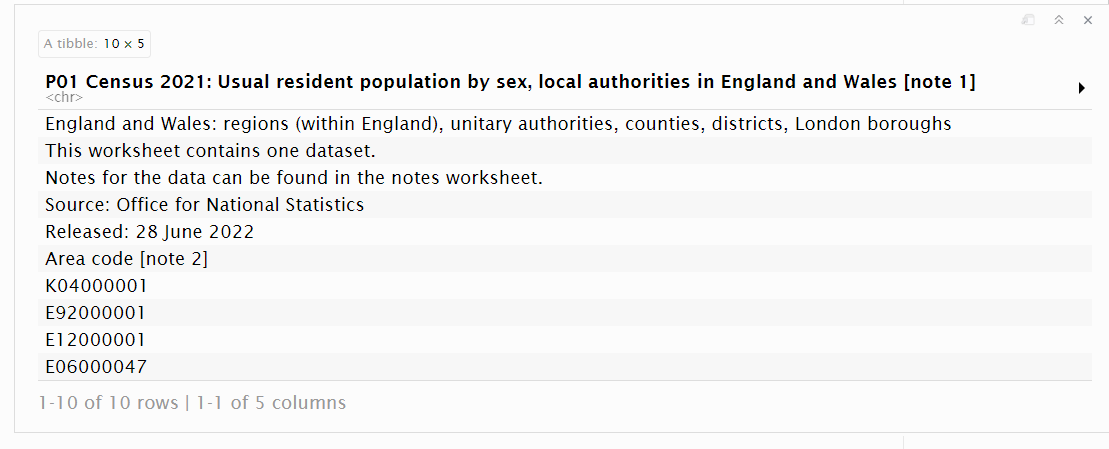
Our focus is on sheet “P01”, with population by sex. The first few rows of the data look like this:

UK Census data.

The {readxl} package’s read_excel() function is the one we want to use. The first item is the path to the file. The function’s default is to read the first sheet in the Excel file, which is not what we want, so we use the sheet = argument to specify “P01”. We will also read only the first 10 rows in the sheet, using the n_max = 10 specification.

uk_census_pop <- readxl::read_excel(
  dpjr::dpjr_data("census2021firstresultsenglandwales1.xlsx"),
  sheet = "P01",
  n_max = 10
)

uk_census_pop

UK Census data.

Our visual inspection had already informed us that the first few rows at the top of the spreadsheet contain the title (now in the variable name row), along with things like the source and the release date. While this documentation is important, it’s not part of the data we want for our analysis.

Another of the read_excel() arguments to specify the rectangular geometry that contains our data is skip =. Because our visual inspection showed us that the header row for the data of interest starts at the seventh row, we will use it to skip the first 6 rows.

uk_census_pop <- readxl::read_excel(
  dpjr::dpjr_data("census2021firstresultsenglandwales1.xlsx"),
  sheet = "P01",
  n_max = 10,
  skip = 6 
)

head(uk_census_pop)

## # A tibble: 6 × 5
##   `Area code [note 2]` `Area name`       `All persons`
##   <chr>                <chr>                     <dbl>
## 1 K04000001            England and Wales      59597300
## 2 E92000001            England                56489800
## 3 E12000001            North East              2647100
## 4 E06000047            County Durham            522100
## 5 E06000005            Darlington               107800
## 6 E06000001            Hartlepool                92300
## # ℹ 2 more variables: Females <dbl>, Males <dbl>

A second option would be to define the range of the cells, using Excel nomenclature to define the upper-left and bottom-right of the data rectangle. This is often a good approach when there is content outside the boundary of the data rectangle, such as additional notes.

Again, opening the file in Excel for a visual scan can provide some valuable insights…here, we can see the additional rows at the top, as well as the hierarchical nature of the data structure.

In this code, we will also apply the clean_names() function from the {janitor} package (Firke 2021), which cleans the variable names. Specifically, it removes the spaces (and any other problematic characters), and puts the variable names into lower case. Finally, the rename() function is applied to remove the “_note_2” text from the area code variable.

uk_census_pop <- readxl::read_excel(
  dpjr::dpjr_data("census2021firstresultsenglandwales1.xlsx"),
  sheet = "P01",
  range = "A7:E382"
) |>
  janitor::clean_names() |>
  rename(area_code = area_code_note_2)

uk_census_pop

## # A tibble: 375 × 5
##    area_code area_name       all_persons females  males
##    <chr>     <chr>                 <dbl>   <dbl>  <dbl>
##  1 K04000001 England and Wa…    59597300  3.04e7 2.92e7
##  2 E92000001 England            56489800  2.88e7 2.77e7
##  3 E12000001 North East          2647100  1.35e6 1.29e6
##  4 E06000047 County Durham        522100  2.67e5 2.55e5
##  5 E06000005 Darlington           107800  5.51e4 5.27e4
##  6 E06000001 Hartlepool            92300  4.77e4 4.47e4
##  7 E06000002 Middlesbrough        143900  7.3 e4 7.09e4
##  8 E06000057 Northumberland       320600  1.64e5 1.57e5
##  9 E06000003 Redcar and Cle…      136500  7.05e4 6.61e4
## 10 E06000004 Stockton-on-Te…      196600  1.00e5 9.65e4
## # ℹ 365 more rows

The data has been read correctly, including the fact that the data variables are read in the correct format. But this loses an important piece of information: the geographical hierarchy. In the Excel file, the levels of the hierarchy are represented by the indentation. Our next challenge is to capture that information as data we can use.

6.2.1 Excel formatting as data

One thing to notice about this data is the Area name variable is hierarchical, with a series of sub-totals. The lower (smaller) levels, containing the component areas of the next higher level in the hierarchy, are represented by indentations in the area name value. The lower the level in the hierarchy, the more indented the name of the area.

The specifics of the hierarchy are as follows:

The value “England and Wales” contains the total population, which is the sum of England (Excel’s row 8) and Wales (row 360).
England (but not Wales) is then further subdivided into nine sub-national Regions (coded as “E12” in the first three characters of the Area code variable).
These Regions are then are divided into smaller units, but the description of those units varies. These are Unitary Authorities (E06), London Boroughs (E09), Counties (E10), and Metropolitan Counties (E11); for our purpose, let’s shorthand this level as “counties”.
The county level is further divided into Non-Metropolitan Districts (E07), and Metropolitan Counties are subdivided into Metropolitan Districts (E08). The image above shows Tyne and Wear (an E11 Met County, at row 18) is subdivided, starting with Gateshead, while Cumbria (an E10 County, at row 31) is also subdivided, starting with Allerdale.
Wales is divided into Unitary Authorities, coded as “W06” in the first three characters of the Area code variable. In Wales, there is no intervening Region, so these are at the same level as the Unitary Authorities in England. ⁸ ⁹

This complicated structure means that the data has multiple subtotals—a sum() function on the All persons variable will lead to a total population of 277,092,700, roughly 4.7 times the actual population of England and Wales in 2021, which was 59,597,300.

What would be much more useful is a structure that has the following characteristics:

No duplication (people aren’t double-counted).
A code for the level of the hierarchy, to enable filtering.
Additional variables (columns), so that each row has the higher level area of which it is a part. For example, County Durham would have a column that contains the regional value “North East” and the country value of “England”.

With that structure, we could use the different regional groupings in a group_by() function.

As we saw earlier, the {readxl} function read_excel() ignores the formatting, so there is no way to discern the level in the characters.

Let’s explore approaches to extracting the information that is embedded in the data and the formatting, and use that to prune the duplicated rows.

Approach 1 - use the Area code

The first approach we can take is to extract the regional element in the area_code variable, and use that to filter the data.

For example, if we want to plot the population in England by the county level, an approach would be to identify all those rows that have an Area code that starts with one of the following:

Unitary Authorities (E06), London Boroughs (E09), Counties (E10), and Metropolitan Counties (E11)

For this, we can design a regular expression that identifies a letter “E” at the beginning by using the “^” character. (Remember, the “E” is for England, and “W” for Wales.) This is then followed by either a 0 or a 1 in the 2nd character spot (within the first set of square brackets), and in the third spot one of 6, 9, 0, or 1 (within the second set of square brackets).

county_pop <- uk_census_pop |> 
  filter(str_detect(area_code, "^E[01][6901]"))

dplyr::glimpse(county_pop, width = 65)

## Rows: 122
## Columns: 5
## $ area_code   <chr> "E06000047", "E06000005", "E06000001", "E06…
## $ area_name   <chr> "County Durham", "Darlington", "Hartlepool"…
## $ all_persons <dbl> 522100, 107800, 92300, 143900, 320600, 1365…
## $ females     <dbl> 266800, 55100, 47700, 73000, 164000, 70500,…
## $ males       <dbl> 255300, 52700, 44700, 70900, 156600, 66100,…

We can check to ensure that the regex has worked as intended through the distinct() function, examining only the first three characters of the area_code strings:

county_pop  |>  
  distinct(str_sub(area_code, 1, 3))

## # A tibble: 4 × 1
##   `str_sub(area_code, 1, 3)`
##   <chr>                     
## 1 E06                       
## 2 E11                       
## 3 E10                       
## 4 E09

Another approach would be to create a list of the desired three-character codes, then create a new variable in the main data, and filter against a list of UA codes:

# create list of UA three-character codes
county_list <- c("E06", "E09", "E10", "E11")

county_pop <- uk_census_pop |> 
  # create three character area prefix
  mutate(area_code_3 = str_sub(area_code, 1, 3)) |> 
  # filter that by the county_list
  filter(area_code_3 %in% county_list)

For our validation checks, we will ensure that our list of UAs is complete, and that the calculated total population matches what is given in the “England” row of the source data:

# check
county_pop  |>  
  distinct(area_code_3)

## # A tibble: 4 × 1
##   area_code_3
##   <chr>      
## 1 E06        
## 2 E11        
## 3 E10        
## 4 E09

# check
county_pop  |>  
  summarize(total_pop = sum(all_persons))

## # A tibble: 1 × 1
##   total_pop
##       <dbl>
## 1  56489600

While this approach works for our particular example, it will require careful coding every time we want to use it. Because of that limited flexibility, we may want to use another approach.

Approach 2 - use Excel’s formatting

The leading space we see when we view the Excel file in its native software is not created by space characters, but through Excel’s “indent” formatting. The {tidyxl} package (Garmonsway et al. 2022) has functions that allow us to turn that formatting into information, which we can then use in the functions within the {unpivotr} package (Garmonsway 2023).

library(tidyxl)
library(unpivotr)

The code below uses the function xlsx_sheet_names() to get the names of all of the sheets in the Excel file.

tidyxl::xlsx_sheet_names(
  dpjr::dpjr_data("census2021firstresultsenglandwales1.xlsx")
  )

## [1] "Cover sheet" "Contents"    "Notes"      
## [4] "P01"         "P02"         "P03"        
## [7] "P04"         "H01"

We already know that Excel files can contain a lot of information that is outside the data rectangle. Rather than ignore all the information that’s in the sheet, we will use the function tidyxl::xlsx_cells() to read the entire sheet. This uses the object with the file path character string and the sheets = argument to specify which one to read. Unlike readxl::read_excel(), we won’t specify the sheet geometry. This will read the contents of the entire sheet, and we will extract the data we want from the object uk_census created at this step.

uk_census <- tidyxl::xlsx_cells(
  dpjr::dpjr_data("census2021firstresultsenglandwales1.xlsx"),
  sheets = "P01"
  )

# take a quick look
dplyr::glimpse(uk_census, width = 65)

## Rows: 1,888
## Columns: 24
## $ sheet               <chr> "P01", "P01", "P01", "P01", "P01", …
## $ address             <chr> "A1", "D1", "A2", "A3", "A4", "A5",…
## $ row                 <int> 1, 1, 2, 3, 4, 5, 6, 6, 7, 7, 7, 7,…
## $ col                 <int> 1, 4, 1, 1, 1, 1, 1, 4, 1, 2, 3, 4,…
## $ is_blank            <lgl> FALSE, TRUE, FALSE, FALSE, FALSE, F…
## $ content             <chr> "97", NA, "98", "99", "100", "101",…
## $ data_type           <chr> "character", "blank", "character", …
## $ error               <chr> NA, NA, NA, NA, NA, NA, NA, NA, NA,…
## $ logical             <lgl> NA, NA, NA, NA, NA, NA, NA, NA, NA,…
## $ numeric             <dbl> NA, NA, NA, NA, NA, NA, NA, NA, NA,…
## $ date                <dttm> NA, NA, NA, NA, NA, NA, NA, NA, NA…
## $ character           <chr> "P01 Census 2021: Usual resident po…
## $ character_formatted <list> [<tbl_df[1 x 14]>], <NULL>, [<tbl_…
## $ formula             <chr> NA, NA, NA, NA, NA, NA, NA, NA, NA,…
## $ is_array            <lgl> FALSE, FALSE, FALSE, FALSE, FALSE, …
## $ formula_ref         <chr> NA, NA, NA, NA, NA, NA, NA, NA, NA,…
## $ formula_group       <int> NA, NA, NA, NA, NA, NA, NA, NA, NA,…
## $ comment             <chr> NA, NA, NA, NA, NA, NA, NA, NA, NA,…
## $ height              <dbl> 19.15, 19.15, 16.90, 15.00, 15.00, …
## $ width               <dbl> 21.71, 12.43, 21.71, 21.71, 21.71, …
## $ row_outline_level   <dbl> 1, 1, 1, 1, 1, 1, 1, 1, 1, 1, 1, 1,…
## $ col_outline_level   <dbl> 1, 1, 1, 1, 1, 1, 1, 1, 1, 1, 1, 1,…
## $ style_format        <chr> "Heading 1", "Normal", "Heading 2",…
## $ local_format_id     <int> 48, 29, 30, 14, 14, 14, 14, 14, 55,…

The dataframe created by the xlsx_cells() function is nothing like the spreadsheet in the Excel file. Instead, every cell in the Excel file is a row, and details about that cell are captured. The cell location is captured in the variable “address”, while there is also a separate variable for the row number and another for the column number. There is also the value we would see if we were to look at the file, in the variable character. (If there is a formula in a cell, the function returns the result of the formula in the character variable, and the text of the formula in the formula variable.)

The local_format_id variable is created by {tidyxlr}, and helps us solve the problem of capturing the indentation. This variable contains a unique value for every different type of formatting that is used in the sheet. Below, we look at the first ten rows of the uk_census object, and we can see that the value “14” appears repeatedly in the variable “local_format_id”.

uk_census |> 
  select(address, character, local_format_id) |> 
  glimpse(width = 65)

## Rows: 1,888
## Columns: 3
## $ address         <chr> "A1", "D1", "A2", "A3", "A4", "A5", "A6…
## $ character       <chr> "P01 Census 2021: Usual resident popula…
## $ local_format_id <int> 48, 29, 30, 14, 14, 14, 14, 14, 55, 55,…

The next thing we need to do is read the details of each of the formats stored in the Excel file—the format “14” has particular characteristics, including the number of indentations in the cell.

For this, we use the {tidyxl} function xlsx_formats(). We only need to specify the path to the file. “Excel defines only one of these dictionaries for the whole workbook, so that it records each combination of formats only once. Two cells that have the same formatting, but are in different sheets, will have the same format code, referring to the same entries in that dictionary.” ¹⁰

The code below reads the formats and assigns the results to a new object uk_census_formats.

uk_census_formats <- xlsx_formats(
  dpjr::dpjr_data("census2021firstresultsenglandwales1.xlsx"),
)

When examining the uk_census_formats object in our environment, we see that it contains two lists, one called “local” and the other “style”. If we look inside “local”, we see one called “alignment”, and within that is “indent”—this is what we’re looking for.

UK Census data.

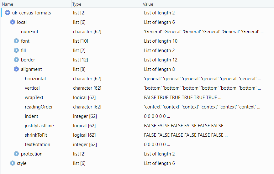
You may have noticed that there are 62 elements in these lists, not 382 (the number of rows in the Excel file), or the 1,888 that represents each active cell in the sheet P01. What the 62 represents is the number of different formats present in the entire Excel file (across all of the sheets).

We can extract that list-within-a-list, which contains all the indentation specifications of the different cell formats in the file, using the code below:

indent <- uk_census_formats$local$alignment$indent
indent

##  [1] 0 0 0 0 0 0 0 0 0 0 0 0 0 0 0 0 0 0 0 0 0 0 0 0 0
## [26] 0 0 0 0 0 0 0 0 0 0 0 0 0 0 0 0 0 0 0 0 0 0 0 0 0
## [51] 0 0 0 0 0 0 0 1 2 4 3 0

This shows that for most of the various cell formattings used in the file most have zero indentation, but some have 1, 2, 3, or 4 indents.

Back to the object uk_census. We are interested in the data starting in the eighth row, so we need to filter for that.

For the {tidyxl} functions to work, the first column needs to define the hierarchical structure. To accomplish this, we will select it out using the != operator.

The behead_if() function identifies a level of headers in a pivot table, and makes it part of the data. Similar to the {tidyr} function pivot_longer(), it creates a new variable for each row based on the headers. In the case of the UK Census data, the headers are differentiated by the number of indents in the formatting.

Let’s test that by assigning the “left-up” position value to a new variable, field0. For each row in the uk_census object, the number of indentations associated with the local_format_id is evaluated; if it’s zero, the following happens: starting at the numeric value, the function looks left and then up until it finds a value that has fewer indentations. For example, the “England” row has a single indentation, so the function looks left and up until it finds a value that has zero indents in the formatting; the value from that cell is assigned to the variable field0 (for zero indents).

uk_census |> 
  dplyr::filter((row >= 7)) |> 
  filter(col != 1) |> 
  behead_if(indent[local_format_id] == 0, 
            direction = "left-up", 
            name = "field0"
            ) |>
  select(address, row, col, content, field0) |> 
  dplyr::filter(row < 30)

## # A tibble: 90 × 5
##    address   row   col content  field0           
##    <chr>   <int> <int> <chr>    <chr>            
##  1 C7          7     3 104      Area name        
##  2 D7          7     4 105      Area name        
##  3 E7          7     5 106      Area name        
##  4 C8          8     3 59597300 England and Wales
##  5 D8          8     4 30420100 England and Wales
##  6 E8          8     5 29177200 England and Wales
##  7 B9          9     2 110      England and Wales
##  8 C9          9     3 56489800 England and Wales
##  9 D9          9     4 28833500 England and Wales
## 10 E9          9     5 27656300 England and Wales
## # ℹ 80 more rows

Let’s continue that through all the levels of indentation. There are four, so we will create a variable that starts with field and then a digit with the number of indentations.

uk_census_behead <- uk_census |> 
  dplyr::filter((row >= 7)) |> 
  filter(col != 1) |> 
  behead_if(indent[local_format_id] == 0, 
            direction = "left-up", name = "field0") |> 
  behead_if(indent[local_format_id] == 1, 
            direction = "left-up", name = "field1") |> 
  behead_if(indent[local_format_id] == 2, 
            direction = "left-up", name = "field2") |> 
  behead_if(indent[local_format_id] == 3, 
            direction = "left-up", name = "field3") |> 
  behead_if(indent[local_format_id] == 4, 
            direction = "left-up", name = "field4")

In the version below, only the final line changes. All of the other indentation values have been evaluated, so it doesn’t require the _if and the associated evaluation, nor does it require the “-up” of the direction.

uk_census_behead <- uk_census |> 
  dplyr::filter((row >= 7)) |> 
  filter(col != 1) |> 
  behead_if(indent[local_format_id] == 0, 
            direction = "left-up", name = "field0") |> 
  behead_if(indent[local_format_id] == 1, 
            direction = "left-up", name = "field1") |> 
  behead_if(indent[local_format_id] == 2, 
            direction = "left-up", name = "field2") |> 
  behead_if(indent[local_format_id] == 3, 
            direction = "left-up", name = "field3") |> 
  behead(direction = "left", name = "field4")

In the code below, the addition is the assignment of column headers. In the UK Census data, the structure is not particularly complex, but {tidyr} can also deal with nested hierarchy in the headers as well.

# from the previous chunk:

uk_census_behead <- uk_census |> 
  dplyr::filter((row >= 7)) |> 
  filter(col != 1) |> 
  behead_if(indent[local_format_id] == 0, 
            direction = "left-up", name = "field0") |> 
  behead_if(indent[local_format_id] == 1, 
            direction = "left-up", name = "field1") |> 
  behead_if(indent[local_format_id] == 2, 
            direction = "left-up", name = "field2") |> 
  behead_if(indent[local_format_id] == 3, 
            direction = "left-up", name = "field3") |> 
  behead(direction = "left", name = "field4") |> 
#  now strip (behead) the column names 
  behead(direction = "up", name = "gender") |> 
# add row sorting to preserve visual comparability  
  arrange(row)

Did we get the results we expected? Let’s do some quick checks of the data, first to see if the 1,125 cells of Excel data (CX to DY) are represented by an individual row (the result of the pivot):

glimpse(uk_census_behead, width = 65)

## Rows: 1,125
## Columns: 30
## $ sheet               <chr> "P01", "P01", "P01", "P01", "P01", …
## $ address             <chr> "C8", "D8", "E8", "C9", "D9", "E9",…
## $ row                 <int> 8, 8, 8, 9, 9, 9, 10, 10, 10, 11, 1…
## $ col                 <int> 3, 4, 5, 3, 4, 5, 3, 4, 5, 3, 4, 5,…
## $ is_blank            <lgl> FALSE, FALSE, FALSE, FALSE, FALSE, …
## $ content             <chr> "59597300", "30420100", "29177200",…
## $ data_type           <chr> "numeric", "numeric", "numeric", "n…
## $ error               <chr> NA, NA, NA, NA, NA, NA, NA, NA, NA,…
## $ logical             <lgl> NA, NA, NA, NA, NA, NA, NA, NA, NA,…
## $ numeric             <dbl> 59597300, 30420100, 29177200, 56489…
## $ date                <dttm> NA, NA, NA, NA, NA, NA, NA, NA, NA…
## $ character           <chr> NA, NA, NA, NA, NA, NA, NA, NA, NA,…
## $ character_formatted <list> <NULL>, <NULL>, <NULL>, <NULL>, <N…
## $ formula             <chr> NA, NA, NA, NA, NA, NA, NA, NA, NA,…
## $ is_array            <lgl> FALSE, FALSE, FALSE, FALSE, FALSE, …
## $ formula_ref         <chr> NA, NA, NA, NA, NA, NA, NA, NA, NA,…
## $ formula_group       <int> NA, NA, NA, NA, NA, NA, NA, NA, NA,…
## $ comment             <chr> NA, NA, NA, NA, NA, NA, NA, NA, NA,…
## $ height              <dbl> 15.6, 15.6, 15.6, 15.6, 15.6, 15.6,…
## $ width               <dbl> 14.71, 12.43, 12.43, 14.71, 12.43, …
## $ row_outline_level   <dbl> 1, 1, 1, 1, 1, 1, 1, 1, 1, 1, 1, 1,…
## $ col_outline_level   <dbl> 1, 1, 1, 1, 1, 1, 1, 1, 1, 1, 1, 1,…
## $ style_format        <chr> "Normal", "Normal", "Normal", "Norm…
## $ local_format_id     <int> 33, 33, 33, 33, 33, 33, 33, 33, 33,…
## $ field0              <chr> "England and Wales", "England and W…
## $ field1              <chr> NA, NA, NA, "England", "England", "…
## $ field2              <chr> NA, NA, NA, NA, NA, NA, "North East…
## $ field3              <chr> NA, NA, NA, NA, NA, NA, NA, NA, NA,…
## $ field4              <chr> NA, NA, NA, NA, NA, NA, NA, NA, NA,…
## $ gender              <chr> "All persons", "Females", "Males", …

We can also look at the first few rows of the variables we are interested in, with a combination of select() and slice_head().

uk_census_behead |> 
  select(field0:field4, gender, numeric) |> 
  slice_head(n = 10)

## # A tibble: 10 × 7
##    field0    field1 field2 field3 field4 gender numeric
##    <chr>     <chr>  <chr>  <chr>  <chr>  <chr>    <dbl>
##  1 England … <NA>   <NA>   <NA>   <NA>   All p…  5.96e7
##  2 England … <NA>   <NA>   <NA>   <NA>   Femal…  3.04e7
##  3 England … <NA>   <NA>   <NA>   <NA>   Males   2.92e7
##  4 England … Engla… <NA>   <NA>   <NA>   All p…  5.65e7
##  5 England … Engla… <NA>   <NA>   <NA>   Femal…  2.88e7
##  6 England … Engla… <NA>   <NA>   <NA>   Males   2.77e7
##  7 England … Engla… North… <NA>   <NA>   All p…  2.65e6
##  8 England … Engla… North… <NA>   <NA>   Femal…  1.35e6
##  9 England … Engla… North… <NA>   <NA>   Males   1.29e6
## 10 England … Engla… North… Count… <NA>   All p…  5.22e5

So far, so good.

And the bottom 10 rows, using slice_tail().

uk_census_behead |> 
  select(field0:field4, gender, numeric) |> 
  slice_tail(n = 10)

## # A tibble: 10 × 7
##    field0    field1 field2 field3 field4 gender numeric
##    <chr>     <chr>  <chr>  <chr>  <chr>  <chr>    <dbl>
##  1 England … Wales  South… Somer… Blaen… Males    32800
##  2 England … Wales  South… Somer… Torfa… All p…   92300
##  3 England … Wales  South… Somer… Torfa… Femal…   47400
##  4 England … Wales  South… Somer… Torfa… Males    44900
##  5 England … Wales  South… Somer… Monmo… All p…   93000
##  6 England … Wales  South… Somer… Monmo… Femal…   47400
##  7 England … Wales  South… Somer… Monmo… Males    45600
##  8 England … Wales  South… Somer… Newpo… All p…  159600
##  9 England … Wales  South… Somer… Newpo… Femal…   81200
## 10 England … Wales  South… Somer… Newpo… Males    78400

Wait! Didn’t we learn that Wales is not divided into regions, and that there are no divisions of the Unitary Authority level? Furthermore, you may also already know that Somerset is in England, not Wales. What’s gone wrong?

A check of the tail of the data (above) reveals a problem with the structure of the Excel file, which (mostly) reflects the nature of the hierarchy. This is not a problem with the {tidyr} and {unpivotr} functions! Those functions are doing things exactly correctly. The values are being pulled from the value that is found at “left-up”.

The first thing that catches my eye is that field2—the Region—should be NA for Wales, but it has been assigned to the South West, which is the last English Region in the data.

More problematically, the Welsh Unitary Authorities (W06) should be in field3, at the same level as the English Unitary Authorities (E06), but instead have been assigned to field4. This has led to Somerset, in England, to be assigned to the column where we expect to see the names of the Welsh Unitary Authorities.

Let’s take a look at the details of the first row of the Welsh Unitary Authorities. First, in the uk_census object, we see that the value of local_format_id for the name (“Isle of Anglesey”) is 60.

uk_census |> 
  dplyr::filter((row == 361)) |> 
  select(address, local_format_id, data_type, character, numeric)

## # A tibble: 5 × 5
##   address local_format_id data_type character   numeric
##   <chr>             <int> <chr>     <chr>         <dbl>
## 1 A361                 11 character W06000001        NA
## 2 B361                 60 character Isle of An…      NA
## 3 C361                 33 numeric   <NA>          68900
## 4 D361                 33 numeric   <NA>          35200
## 5 E361                 33 numeric   <NA>          33700

We can then use this to examine the details of the indent formatting, which we captured in the formats object.

uk_census_formats$local$alignment$indent[60]

## [1] 4

There are 4 indents. You will recall that the behead_if() function was looking left and up. In the case of the Welsh entries, the function has looked left and up until it found an entry that has fewer indents, which happens to be in England, not Wales.

This problem has arisen at the transition from one area to the next. Did this also happen in the England rows, for example where the North West region row appears? As we can see below, as similar problem has occurred: the value “North West” is correctly assigned to field2, but field3 has been populated with the first value above North West where there is a valid value in field3.

uk_census_behead |> 
  select(address, content, field0, field1, field2, field3, field4) |> 
  filter(field2 == "North West")

## # A tibble: 132 × 7
##    address content field0   field1 field2 field3 field4
##    <chr>   <chr>   <chr>    <chr>  <chr>  <chr>  <chr> 
##  1 C24     7417300 England… Engla… North… Tyne … <NA>  
##  2 D24     3777200 England… Engla… North… Tyne … <NA>  
##  3 E24     3640100 England… Engla… North… Tyne … <NA>  
##  4 C25     154800  England… Engla… North… Black… <NA>  
##  5 D25     78100   England… Engla… North… Black… <NA>  
##  6 E25     76800   England… Engla… North… Black… <NA>  
##  7 C26     141100  England… Engla… North… Black… <NA>  
##  8 D26     71400   England… Engla… North… Black… <NA>  
##  9 E26     69700   England… Engla… North… Black… <NA>  
## 10 C27     398800  England… Engla… North… Chesh… <NA>  
## # ℹ 122 more rows

Now that we have diagnosed the problem, what solution can we apply?

One solution is to repopulate each level’s field variable by stepping up a level and comparing that to the value three rows earlier in the data.¹¹ (We look at the previous rows using the dplyr::lag() function. It has to be three rows because our beheading function has made separate rows for “All persons”, “Female”, and “Male”.)

If the prior field is not the same, it gets replaced with an “NA”, but if it’s the same, then the current value is retained. In the first mutate() function, field1 is replaced if field0 in the current spot is not the same as the field0 three rows prior.

uk_census_behead |> 
  select(row, col, starts_with("field")) |>
  arrange(row, col) |>
  mutate(field1 = if_else(field0 == lag(field0, n = 3), field1, NA)) |>
  mutate(field2 = if_else(field1 == lag(field1, n = 3), field2, NA)) |>
  mutate(field3 = if_else(field2 == lag(field2, n = 3), field3, NA)) |>
  mutate(field4 = if_else(field3 == lag(field3, n = 3), field4, NA))

## # A tibble: 1,125 × 7
##      row   col field0       field1 field2 field3 field4
##    <int> <int> <chr>        <chr>  <chr>  <chr>  <chr> 
##  1     8     3 England and… <NA>   <NA>   <NA>   <NA>  
##  2     8     4 England and… <NA>   <NA>   <NA>   <NA>  
##  3     8     5 England and… <NA>   <NA>   <NA>   <NA>  
##  4     9     3 England and… Engla… <NA>   <NA>   <NA>  
##  5     9     4 England and… Engla… <NA>   <NA>   <NA>  
##  6     9     5 England and… Engla… <NA>   <NA>   <NA>  
##  7    10     3 England and… Engla… North… <NA>   <NA>  
##  8    10     4 England and… Engla… North… <NA>   <NA>  
##  9    10     5 England and… Engla… North… <NA>   <NA>  
## 10    11     3 England and… Engla… North… Count… <NA>  
## # ℹ 1,115 more rows

Unfortunately, this solution does not repair the mis-assignment of the UAs in Wales.

In the code below, the values in field1 are evaluated. For those with population data from Wales, the field2 and field3 values are replaced with an NA.

uk_census_behead_revised <- uk_census_behead |> 
  mutate(field2 = case_when(
    field1 == "Wales" ~ NA_character_,
    TRUE ~ field2
  )) |>
  mutate(field3 = case_when(
    field1 == "Wales" ~ NA_character_,
    TRUE ~ field3
  )) |>
  select(field0:field4, gender, numeric)
  
uk_census_behead_revised |> 
  tail()

## # A tibble: 6 × 7
##   field0     field1 field2 field3 field4 gender numeric
##   <chr>      <chr>  <chr>  <chr>  <chr>  <chr>    <dbl>
## 1 England a… Wales  <NA>   <NA>   Monmo… All p…   93000
## 2 England a… Wales  <NA>   <NA>   Monmo… Femal…   47400
## 3 England a… Wales  <NA>   <NA>   Monmo… Males    45600
## 4 England a… Wales  <NA>   <NA>   Newpo… All p…  159600
## 5 England a… Wales  <NA>   <NA>   Newpo… Femal…   81200
## 6 England a… Wales  <NA>   <NA>   Newpo… Males    78400

In many uses of this data, we will want to remove the subtotal rows. In the code below, a case_when() function is applied to create a new variable that contains a value “subtotal” for the rows that are disaggregated at the next level (for example, the cities within a Metro county, or the counties within a region).

The first step is to create a new dataframe field3_split that identifies all of the areas at the county level that have a dissaggregation. This is done by first filtering by field4, where there is a valid value (identified as not an “NA”), and creating a list of the distinct values in field3. That list is then used as part of the evaluation within the case_when() to assign the value “subtotal” to the new variable subtotal_row.

field3_split <- uk_census_behead_revised |> 
  filter(!is.na(field4)) |> 
  distinct(field3)  
  
field3_split

## # A tibble: 33 × 1
##    field3                         
##    <chr>                          
##  1 Tyne and Wear (Met County)     
##  2 Cumbria                        
##  3 Greater Manchester (Met County)
##  4 Lancashire                     
##  5 Merseyside (Met County)        
##  6 North Yorkshire                
##  7 South Yorkshire (Met County)   
##  8 West Yorkshire (Met County)    
##  9 Derbyshire                     
## 10 Leicestershire                 
## # ℹ 23 more rows

uk_census_behead_revised |> 
  mutate(subtotal_row = case_when(
    field3 %in% field3_split$field3 & is.na(field4) ~ "subtotal",
    TRUE ~ NA_character_
    )) |> 
  relocate(subtotal_row)

## # A tibble: 1,125 × 8
##    subtotal_row field0      field1 field2 field3 field4
##    <chr>        <chr>       <chr>  <chr>  <chr>  <chr> 
##  1 subtotal     England an… <NA>   <NA>   <NA>   <NA>  
##  2 subtotal     England an… <NA>   <NA>   <NA>   <NA>  
##  3 subtotal     England an… <NA>   <NA>   <NA>   <NA>  
##  4 subtotal     England an… Engla… <NA>   <NA>   <NA>  
##  5 subtotal     England an… Engla… <NA>   <NA>   <NA>  
##  6 subtotal     England an… Engla… <NA>   <NA>   <NA>  
##  7 subtotal     England an… Engla… North… <NA>   <NA>  
##  8 subtotal     England an… Engla… North… <NA>   <NA>  
##  9 subtotal     England an… Engla… North… <NA>   <NA>  
## 10 <NA>         England an… Engla… North… Count… <NA>  
## # ℹ 1,115 more rows
## # ℹ 2 more variables: gender <chr>, numeric <dbl>

Approach 3 - build a concordance table

If we need a more flexible and re-usable approach, we can consider the option of creating a separate concordance table (also known as a crosswalk table). A table of this sort contains the distinct values of key variables and their corresponding values in another typology or schema. Once a table like this is built, it can be joined to our data, as well as to any other table we might need to use in the future.

For the UK Census data, we will create two separate concordance tables. We will save these tables as CSV files, so they are readily available for other instances when their use will make filtering and summarizing the data more efficient.

For the first table, we will build a table with each type of administrative region and its associated three-digit code. This is done programatically in R, using the {tibble} package (Müller and Wickham 2021). We will use the tribble() function, which transposes the layout so it resembles the final tabular structure.

In addition to the area code prefix and the name of the administrative region type, the level in the hierarchy is also encoded in this table.

uk_region_table <- tribble(
  # header row
  ~"area_code_3", ~"category", ~"geo_level",
  "K04", "England & Wales", 0,
  "E92", "England", 1,
  "E12", "Region", 2,
  "E09", "London Borough", 3,
  "E10", "County",  3,
  "E07", "Non-Metropolitan District", 4,
  "E06", "Unitary Authority", 3,
  "E11", "Metropolitan County", 3,
  "E08", "Metropolitan District", 4,
  "W92", "Wales", 1,
  "W06", "Unitary Authority", 3
)

uk_region_table

## # A tibble: 11 × 3
##    area_code_3 category                  geo_level
##    <chr>       <chr>                         <dbl>
##  1 K04         England & Wales                   0
##  2 E92         England                           1
##  3 E12         Region                            2
##  4 E09         London Borough                    3
##  5 E10         County                            3
##  6 E07         Non-Metropolitan District         4
##  7 E06         Unitary Authority                 3
##  8 E11         Metropolitan County               3
##  9 E08         Metropolitan District             4
## 10 W92         Wales                             1
## 11 W06         Unitary Authority                 3

This table can be saved as a CSV file for future reference:

write_csv(uk_region_table, "data_output/uk_region_table.csv")

Our next step is to use a mutate() function to extract the unique values in the area code variable in the dataframe uk_census_pop, and then use that new variable to join the dataframe to the uk_region_table created in the previous chunk.

uk_census_pop_geo <- uk_census_pop |> 
#  select(area_code, area_name) |> 
  mutate(area_code_3 = str_sub(uk_census_pop$area_code, 1, 3)) |> 
  # join with classification table
  left_join(
    uk_region_table,
    by = c("area_code_3" = "area_code_3")
    )

glimpse(uk_census_pop_geo, width = 65)

## Rows: 375
## Columns: 8
## $ area_code   <chr> "K04000001", "E92000001", "E12000001", "E06…
## $ area_name   <chr> "England and Wales", "England", "North East…
## $ all_persons <dbl> 59597300, 56489800, 2647100, 522100, 107800…
## $ females     <dbl> 30420100, 28833500, 1353800, 266800, 55100,…
## $ males       <dbl> 29177200, 27656300, 1293300, 255300, 52700,…
## $ area_code_3 <chr> "K04", "E92", "E12", "E06", "E06", "E06", "…
## $ category    <chr> "England & Wales", "England", "Region", "Un…
## $ geo_level   <dbl> 0, 1, 2, 3, 3, 3, 3, 3, 3, 3, 3, 4, 4, 4, 4…

Because the level is now encoded in the relevant rows of the dataframe, it is possible to filter on the level variable to calculate the total population for England and Wales.

uk_census_pop_geo |> 
  filter(geo_level == 3) |> 
  summarize(total_population = sum(all_persons))

## # A tibble: 1 × 1
##   total_population
##              <dbl>
## 1         59597300

A more complex concordance table can be derived from the beheaded table we created earlier. The two steps in this process are:

Select the field variables and then create a table with only the distinct values across all the rows,
Create a new variable “area_name” with the lowest-level value, i.e. the values in the source table column B.

uk_census_geo_code <- uk_census_behead_revised |> 
  # select field variables
  select(contains("field")) |> 
  distinct() |> 
  # create variable with lowest-level value
  mutate(area_name = case_when(
    !is.na(field4) ~ field4,
    !is.na(field3) ~ field3,
    !is.na(field2) ~ field2,
    !is.na(field1) ~ field1,
    !is.na(field0) ~ field0,
    TRUE ~ NA_character_
  ))
  

uk_census_geo_code

## # A tibble: 375 × 6
##    field0         field1 field2 field3 field4 area_name
##    <chr>          <chr>  <chr>  <chr>  <chr>  <chr>    
##  1 England and W… <NA>   <NA>   <NA>   <NA>   England …
##  2 England and W… Engla… <NA>   <NA>   <NA>   England  
##  3 England and W… Engla… North… <NA>   <NA>   North Ea…
##  4 England and W… Engla… North… Count… <NA>   County D…
##  5 England and W… Engla… North… Darli… <NA>   Darlingt…
##  6 England and W… Engla… North… Hartl… <NA>   Hartlepo…
##  7 England and W… Engla… North… Middl… <NA>   Middlesb…
##  8 England and W… Engla… North… North… <NA>   Northumb…
##  9 England and W… Engla… North… Redca… <NA>   Redcar a…
## 10 England and W… Engla… North… Stock… <NA>   Stockton…
## # ℹ 365 more rows

The third step is to join the area code variable from the uk_census_pop table.

uk_census_geo_code <- uk_census_geo_code |> 
  left_join(
    select(uk_census_pop, area_name, area_code),
    by = "area_name"
    ) |> 
  relocate(area_name, area_code)

uk_census_geo_code

## # A tibble: 375 × 7
##    area_name      area_code field0 field1 field2 field3
##    <chr>          <chr>     <chr>  <chr>  <chr>  <chr> 
##  1 England and W… K04000001 Engla… <NA>   <NA>   <NA>  
##  2 England        E92000001 Engla… Engla… <NA>   <NA>  
##  3 North East     E12000001 Engla… Engla… North… <NA>  
##  4 County Durham  E06000047 Engla… Engla… North… Count…
##  5 Darlington     E06000005 Engla… Engla… North… Darli…
##  6 Hartlepool     E06000001 Engla… Engla… North… Hartl…
##  7 Middlesbrough  E06000002 Engla… Engla… North… Middl…
##  8 Northumberland E06000057 Engla… Engla… North… North…
##  9 Redcar and Cl… E06000003 Engla… Engla… North… Redca…
## 10 Stockton-on-T… E06000004 Engla… Engla… North… Stock…
## # ℹ 365 more rows
## # ℹ 1 more variable: field4 <chr>

To this table the geographic level values are added by joining the uk_region_table created earlier.

uk_census_geo_code <- uk_census_geo_code |> 
#  select(area_code, area_name) |> 
  mutate(area_code_3 = str_sub(uk_census_pop$area_code, 1, 3)) |> 
  # join with classification table
  left_join(
    uk_region_table,
    by = c("area_code_3" = "area_code_3")
    )

uk_census_geo_code

## # A tibble: 375 × 10
##    area_name      area_code field0 field1 field2 field3
##    <chr>          <chr>     <chr>  <chr>  <chr>  <chr> 
##  1 England and W… K04000001 Engla… <NA>   <NA>   <NA>  
##  2 England        E92000001 Engla… Engla… <NA>   <NA>  
##  3 North East     E12000001 Engla… Engla… North… <NA>  
##  4 County Durham  E06000047 Engla… Engla… North… Count…
##  5 Darlington     E06000005 Engla… Engla… North… Darli…
##  6 Hartlepool     E06000001 Engla… Engla… North… Hartl…
##  7 Middlesbrough  E06000002 Engla… Engla… North… Middl…
##  8 Northumberland E06000057 Engla… Engla… North… North…
##  9 Redcar and Cl… E06000003 Engla… Engla… North… Redca…
## 10 Stockton-on-T… E06000004 Engla… Engla… North… Stock…
## # ℹ 365 more rows
## # ℹ 4 more variables: field4 <chr>, area_code_3 <chr>,
## #   category <chr>, geo_level <dbl>

Now we have a comprehensive table, with all 375 of the administrative geography areas, including the name, area code, and all of the details of the hierarchy.

This table could also be joined to the contents of a population sheet, to provide additional detail.

Let’s imagine your assignment is to determine which region at the UA level has the highest proportion of people aged 90 or older. The code below reads the contents of sheet “P02” in the census population file, which has age detail of the population in each area. By appending the contents of the concordance table, a detailed disaggregation without double counting is possible.

In addition to changing the sheet reference, the code also changes the range to reflect the differences in the contents.

uk_census_pop_90 <- readxl::read_excel(
  dpjr::dpjr_data("census2021firstresultsenglandwales1.xlsx"),
  sheet = "P02",
  range = "A8:V383"
) |> 
  janitor::clean_names() |> 
  dplyr::rename(area_code = area_code_note_2) |> 
  # remove "_note_12" from population variables
  dplyr::rename_with(~str_remove(., "_note_12"))

head(uk_census_pop_90)

## # A tibble: 6 × 22
##   area_code area_name         all_persons
##   <chr>     <chr>                   <dbl>
## 1 K04000001 England and Wales    59597300
## 2 E92000001 England              56489800
## 3 E12000001 North East            2647100
## 4 E06000047 County Durham          522100
## 5 E06000005 Darlington             107800
## 6 E06000001 Hartlepool              92300
## # ℹ 19 more variables: aged_4_years_and_under <dbl>,
## #   aged_5_to_9_years <dbl>,
## #   aged_10_to_14_years <dbl>,
## #   aged_15_to_19_years <dbl>,
## #   aged_20_to_24_years <dbl>,
## #   aged_25_to_29_years <dbl>,
## #   aged_30_to_34_years <dbl>, …

The filter() step below does the following:

selects the area code and the population categories of interest,
joins the detailed geographic descriptions,
filters the level 3 values, but this leaves those UA regions that are further disaggregated into the city category.

uk_census_pop_90 <- uk_census_pop_90 |>
  select(area_code, all_persons, aged_90_years_and_over) |>
  full_join(uk_census_geo_code, by = "area_code") |>
  # filter so that only UAs remain
  filter(geo_level == 3)

With this table, the proportion of persons aged 90 or older can be calculated and the table sorted in descending order:

uk_census_pop_90 |> 
  mutate(
    pct_90_plus = 
      round((aged_90_years_and_over / all_persons * 100), 1)
    ) |> 
  arrange(desc(pct_90_plus)) |> 
  select(area_name, aged_90_years_and_over, pct_90_plus) |> 
  slice_head(n = 10)

## # A tibble: 10 × 3
##    area_name         aged_90_years_and_over pct_90_plus
##    <chr>                              <dbl>       <dbl>
##  1 Dorset [note 10]                    6300         1.7
##  2 East Sussex                         8100         1.5
##  3 Conwy                               1700         1.5
##  4 Isle of Wight                       2000         1.4
##  5 Torbay                              2000         1.4
##  6 Devon                              11200         1.4
##  7 Herefordshire, C…                   2400         1.3
##  8 West Sussex                        11900         1.3
##  9 Bournemouth, Chr…                   5400         1.3
## 10 North Somerset                      2800         1.3

References

Broman, Karl, and Kara Woo. 2017. “Data Organization in Spreadsheets.” The American Statistician 72 (1): 2–10. https://doi.org/10.1080/00031305.2017.1375989.

Bryan, Jenny. 2016a. “Sanesheets.” https://github.com/jennybc/sanesheets.

———. 2016b. “Spreadsheets.” https://github.com/jennybc/2016-06_spreadsheets.

Firke, Sam. 2021. janitor: Simple Tools for Examining and Cleaning Dirty Data. https://github.com/sfirke/janitor.

Garmonsway, Duncan. 2023. unpivotr: Unpivot Complex and Irregular Data Layouts. https://CRAN.R-project.org/package=unpivotr.

Garmonsway, Duncan, Hadley Wickham, Jenny Bryan, RStudio, and Marcin Kalicinski. 2022. tidyxl: ERead Untidy Excel Files. https://CRAN.R-project.org/package=tidyxl.

Müller, Kirill, and Hadley Wickham. 2021. tibble: Simple Data Frames. https://CRAN.R-project.org/package=tibble.

Murrell, Paul. 2013. “Data Intended for Human Consumption, Not Machine Consumption.” In Bad Data Handbook, edited by Q. Ethan McCallum, 31–51. O’Reilly.

Wickham, Hadley, and Jennifer Bryan. 2019. readxl: Read Excel Files. https://CRAN.R-project.org/package=readxl.

For more options, see the “Sheet Geometry” page at the {readxl} site.↩︎
The hierarchy of the administrative geographies of the UK can be found at the “England” and “Wales” links on [the ONS “Administrative geographies” page] (https://www.ons.gov.uk/methodology/geography/ukgeographies/administrativegeography).↩︎
You can download a map of these regions at “Local Authority Districts, Counties and Unitary Authorities (April 2021) Map in United Kingdom”.↩︎
Duncan Garmonsway, response to issue #84, {tidyxl} package repository, 2022-05-26. https://github.com/nacnudus/tidyxl/issues/84 ↩︎
Thanks to Duncan Garmonsway, the author of the {tidyxl} and {untidyr} packages, for the path to this solution.↩︎