9 Terminal shoot analyses
9.1 Goals
Does severing affect the number and size of active, independent rhizome systems?
There are two components of this:
- how does severing affect the number of plants that produce 0, 1, or 2 systems? Approach: contingency table analysis. For each treatment (C, S1, S2, S4), we want to see how many plants had 0, 1, or 2 systems, and compare those counts.
KE thoughts July 14: I think this still makes sense to do. It addresses the question, and this type of analysis doesn’t feel repetitive with other things, because we haven’t been counting systems for the other questions.
- how does severing affect the size of plants that produce 0, 1, or 2 systems? Approach: modeling total leaf area as a function of severing (C, S1, S2, S4), number of systems (0, 1, 2), and their interaction. I know previously we had been talking about breaking the controls out as a separate group. However, I think if we do it this way, it will be more parallel with the contingency table analysis, and lets us test for that interaction, because now our controls won’t be synonymous with both a treatment and a number of systems.
KE thoughts July 14: For this piece, I think working with the zero systems doesn’t make a lot of sense, because they have zero leaf area by definition, and so contrasts with the other categories aren’t super meaningful in general, and also do not vary across the severing treatments, which is the point of this. In the contingency table analysis described above, we can look at how the distribution of the zero systems may vary across the severing treatments. I think the comparisons that are valuable are, within a severing treatment, do systems have different total or average leaf areas when they have a front vs. a back vs. both system components? Putting aside the control treatment, I think for the three types of severing, we should definitely be able to compare front to both. Comparisons involving the back are likely to be non-significant because of the small sample sizes.
So, continuing to think this through, maybe for this portion, comparisons that would be interesting are: control vs. any type of severing for front, back, and both (in reality, this will probably only end up working for the front), and then within s1, s2, and s4, are there differences between front, back, or both? I recognize the first piece is somewhat repetitive with previous analyses of front leaf area, but I think it makes sense to be to present it that way in this context.
Then, what remains to be seen is whether total or average leaf area is a better way of addressing our question. Given the word “independent” in the question above, I think that suggests that we’d want to focus on average leaf area, but I still think that we want to include total leaf area (perhaps as inset plots) because I think it’s helpful to have that visualization.
Both of these analyses can be performed with both the 1991 data and the 1992 data.
A potential extension is incorporating branch number. A simple way to do this would be to use branch number in place of the number of systems. So, in piece a., we would be looking at severing across branch numbers, and for piece b., we would be looking at leaf area as a function of severing, number of branches, and their interaction. I think a potential issue for this is that the contingency table for severing treatment x branch number would be quite large. Another option could be to add branching number as a covariate in the model of leaf area, in addition to the system number x severing treatment interaction.
9.2 Data
Here is the full dataset that will be used for both analyses:
# set na.strings="." to recode '.' to NA
mayappleDatasetFull<-readxl::read_excel("~/Box/Mayapple/Datasets/mayapple_1990_updated_version2.xlsx", na=".")
Check variable names, select relevant variables, convert variables to numeric with parse_double, and remove rows that don’t have a leaf area record for 1990, 1991, or 1992.
#names(mayappleDatasetFull)

#selecting variables of interest, correctly parsing variables, making new variable that sums front and back branch number in each year
mayappleData91 <- mayappleDatasetFull %>%
  dplyr::select(COLONY,Lf_90,Sex_90,Sever,Time,
                LfFtot_91, LfBtot_91, Lftot_91,
                LftotF_92, LftotB_92, Lftot_92,
                brnoF_91, brnoB_91,
                brnoF_92, brnoB_92) %>%
  mutate(Lftot_92=parse_double(Lftot_92), Lftot_91=parse_double(Lftot_91)) %>%
  mutate(LftotB_92=parse_double(LftotB_92), LfBtot_91=parse_double(LfBtot_91) ) %>%
  mutate(LftotF_92=parse_double(LftotF_92), LfFtot_91=parse_double(LfFtot_91) ) %>%
  mutate(brnoF_92=parse_double(brnoF_92), brnoB_92=parse_double(brnoB_92) ) %>%
  filter(!is.na(Lf_90)) %>%
  filter(!is.na(Lftot_91)) %>%
  mutate(brnoT_91=brnoF_91+brnoB_91, brnoT_92=brnoF_92+brnoB_92)

# now we can take the 91 dataset and further filter it for rows that didn't have a leaf area in 1992. This will be the 1992 dataset
mayappleData92 <- mayappleData91 %>%
  filter(!is.na(Lftot_92))
9.3 1991 with 0-1-2
9.3.1 1991 tables
A table of system status (One = front system or back only, Two = front & back, None = dead (no front, no back)) first in total, and then across the treatments:
mayappleData91 %>% mutate(Status = case_when(LfFtot_91!=0 & LfBtot_91!=0 ~"Two",
                                             LfFtot_91==0 & LfBtot_91!=0 ~"One",
                                             LfFtot_91!=0 & LfBtot_91==0 ~"One",
                                             LfFtot_91==0 & LfBtot_91==0 ~"None")) %>%
  group_by(Status) %>%
  summarise(N=length(Sever)) %>%
kable()| Status | N |
|---|---|
| None | 41 |
| One | 291 |
| Two | 117 |
Most systems have only one system.
mayappleData91 %>% mutate(Status = case_when(LfFtot_91!=0 & LfBtot_91!=0 ~"Two",
                                             LfFtot_91==0 & LfBtot_91!=0 ~"One",
                                             LfFtot_91!=0 & LfBtot_91==0 ~"One",
                                             LfFtot_91==0 & LfBtot_91==0 ~"None")) %>%
  group_by(Sever,Status) %>%
  summarise(N=length(Sever)) %>%
kable()| Sever | Status | N |
|---|---|---|
| C | None | 7 |
| C | One | 123 |
| C | Two | 1 |
| S1 | None | 15 |
| S1 | One | 27 |
| S1 | Two | 52 |
| S2 | None | 8 |
| S2 | One | 50 |
| S2 | Two | 45 |
| S4 | None | 11 |
| S4 | One | 91 |
| S4 | Two | 19 |
9.3.2 1991 contingency table analysis:
mayappleData91 <- mayappleData91 %>% mutate(Status = case_when(LfFtot_91!=0 & LfBtot_91!=0 ~"Two",
                                             LfFtot_91==0 & LfBtot_91!=0 ~"One",
                                             LfFtot_91!=0 & LfBtot_91==0 ~"One",
                                             LfFtot_91==0 & LfBtot_91==0 ~"None")) %>%
  mutate(Status = factor(Status, levels=c("None", "One", "Two")))

chisq.test(mayappleData91$Status, mayappleData91$Sever)
##
## Pearson's Chi-squared test
##
## data: mayappleData91$Status and mayappleData91$Sever
## X-squared = 129.59, df = 6, p-value < 2.2e-16## mayappleData91$Sever
## mayappleData91$Status C S1 S2 S4
## None 7 15 8 11
## One 123 27 50 91
## Two 1 52 45 19## mayappleData91$Sever
## mayappleData91$Status C S1 S2 S4
## None 11.96214 8.583519 9.405345 11.04900
## One 84.90200 60.922049 66.755011 78.42094
## Two 34.13586 24.494432 26.839644 31.53007## mayappleData91$Sever
## mayappleData91$Status C S1 S2 S4
## None -1.43471104 2.19010145 -0.45824280 -0.01474059
## One 4.13469192 -4.34605108 -2.05070308 1.42047089
## Two -5.67143299 5.55759544 3.50538717 -2.231469439.3.3 1991 leaf area analysis per system
mayappleData91 <- mayappleData91 %>% mutate(Status = case_when(LfFtot_91!=0 & LfBtot_91!=0 ~"Two",
                                             LfFtot_91==0 & LfBtot_91!=0 ~"One",
                                             LfFtot_91!=0 & LfBtot_91==0 ~"One",
                                             LfFtot_91==0 & LfBtot_91==0 ~"None")) %>%
  mutate(Status = factor(Status, levels=c("None", "One", "Two"))) %>%
  filter(Status != "None")


mayappleData91 <- mayappleData91 %>% mutate(Lf91s=ifelse(Status=="Two", Lftot_91/2, Lftot_91))


s91mod2<-lmer(Lf91s~Status*Sever+(1|COLONY), data = mayappleData91)
anova(s91mod2)
## Type III Analysis of Variance Table with Satterthwaite's method
## Sum Sq Mean Sq NumDF DenDF F value Pr(>F)
## Status 327401 327401 1 391.79 7.3313 0.007073 **
## Sever 285397 95132 3 391.44 2.1302 0.095888 .
## Status:Sever 534833 178278 3 393.68 3.9921 0.008054 **
## ---
## Signif. codes: 0 '***' 0.001 '**' 0.01 '*' 0.05 '.' 0.1 ' ' 1## $emmeans
## Status emmean SE df lower.CL upper.CL
## One 487 17.6 66.5 452 522
## Two 330 56.9 396.3 219 442
##
## Results are averaged over the levels of: Sever
## Degrees-of-freedom method: satterthwaite
## Confidence level used: 0.95
##
## $contrasts
## contrast estimate SE df t.ratio p.value
## One - Two 157 57.9 392 2.708 0.0071
##
## Results are averaged over the levels of: Sever
## Degrees-of-freedom method: satterthwaite## $emmeans
## Status = One:
## Sever emmean SE df lower.CL upper.CL
## C 637 21.4 135 595 679
## S1 336 42.7 356 252 420
## S2 438 31.7 300 376 501
## S4 537 24.3 186 489 585
##
## Status = Two:
## Sever emmean SE df lower.CL upper.CL
## C 210 214.8 395 -212 632
## S1 370 31.4 274 308 432
## S2 392 33.5 303 326 458
## S4 349 50.2 386 250 448
##
## Degrees-of-freedom method: satterthwaite
## Confidence level used: 0.95
##
## $contrasts
## Status = One:
## contrast estimate SE df t.ratio p.value
## C - S1 300.6 45.8 397 6.570 <.0001
## C - S2 198.5 35.8 392 5.538 <.0001
## C - S4 99.5 29.4 386 3.380 0.0044
## S1 - S2 -102.1 51.3 395 -1.992 0.1929
## S1 - S4 -201.2 47.3 398 -4.257 0.0002
## S2 - S4 -99.1 37.6 390 -2.637 0.0430
##
## Status = Two:
## contrast estimate SE df t.ratio p.value
## C - S1 -160.1 216.7 394 -0.739 0.8815
## C - S2 -181.7 217.2 395 -0.837 0.8369
## C - S4 -139.0 220.4 395 -0.631 0.9222
## S1 - S2 -21.7 43.5 391 -0.498 0.9595
## S1 - S4 21.1 57.0 385 0.370 0.9827
## S2 - S4 42.8 58.4 389 0.732 0.8840
##
## Degrees-of-freedom method: satterthwaite
## P value adjustment: tukey method for comparing a family of 4 estimates## $emmeans
## Sever = C:
## Status emmean SE df lower.CL upper.CL
## One 637 21.4 135 595 679
## Two 210 214.8 395 -212 632
##
## Sever = S1:
## Status emmean SE df lower.CL upper.CL
## One 336 42.7 356 252 420
## Two 370 31.4 274 308 432
##
## Sever = S2:
## Status emmean SE df lower.CL upper.CL
## One 438 31.7 300 376 501
## Two 392 33.5 303 326 458
##
## Sever = S4:
## Status emmean SE df lower.CL upper.CL
## One 537 24.3 186 489 585
## Two 349 50.2 386 250 448
##
## Degrees-of-freedom method: satterthwaite
## Confidence level used: 0.95
##
## $contrasts
## Sever = C:
## contrast estimate SE df t.ratio p.value
## One - Two 426.6 215.5 394 1.980 0.0484
##
## Sever = S1:
## contrast estimate SE df t.ratio p.value
## One - Two -34.1 51.5 400 -0.662 0.5083
##
## Sever = S2:
## contrast estimate SE df t.ratio p.value
## One - Two 46.3 44.4 399 1.044 0.2971
##
## Sever = S4:
## contrast estimate SE df t.ratio p.value
## One - Two 188.2 54.3 397 3.465 0.0006
##
## Degrees-of-freedom method: satterthwaiteemmip(s91mod2, Status~Sever,CIs = TRUE)+ ggtitle("Average leaf area per system in 1991")+
theme_bw()+theme(plot.title = element_text(face="italic"))+theme(panel.grid.major = element_blank(), panel.grid.minor = element_blank())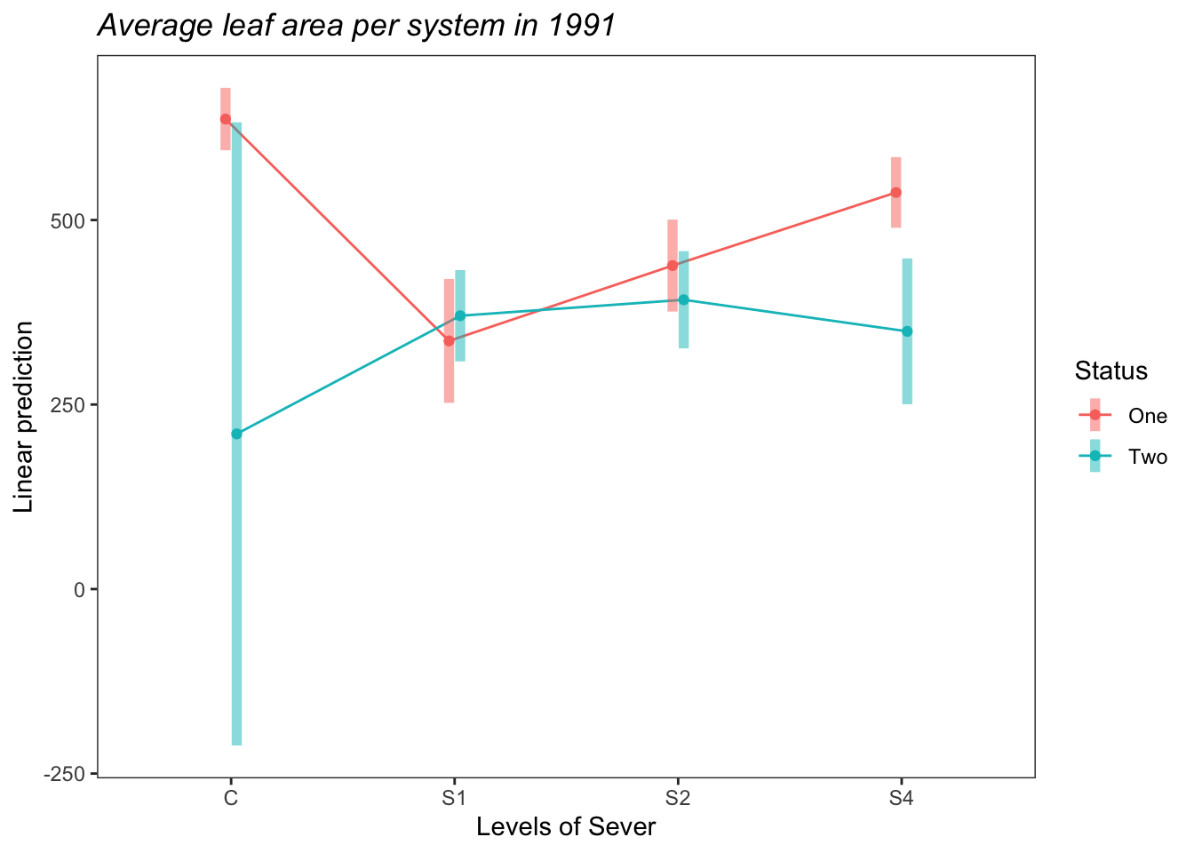
b<-emmip(s91mod2, Sever~Status  ,CIs = TRUE)+ ggtitle("Average leaf area per system in 1991")+
  theme_bw()+theme(plot.title = element_text(face="italic"))+theme(panel.grid.major = element_blank(), panel.grid.minor = element_blank())

b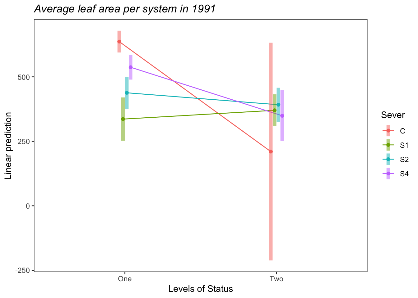
9.4 1992 with 0-1-2
9.4.1 1992 tables
A table of system status (One = front system or back only, Two = front & back, None = dead (no front, no back)) first in total, and then across the treatments:
mayappleData92 %>% mutate(Status = case_when(LftotF_92!=0 & LftotB_92!=0 ~"Two",
                                             LftotF_92==0 & LftotB_92!=0 ~"One",
                                             LftotF_92!=0 & LftotB_92==0 ~"One",
                                             LftotF_92==0 & LftotB_92==0 ~"None")) %>%
  group_by(Status) %>%
  summarise(N=length(Sever)) %>%
kable()| Status | N |
|---|---|
| None | 19 |
| One | 120 |
| Two | 83 |
Most systems have only one system.
mayappleData92 %>% mutate(Status = case_when(LftotF_92!=0 & LftotB_92!=0 ~"Two",
                                             LftotF_92==0 & LftotB_92!=0 ~"One",
                                             LftotF_92!=0 & LftotB_92==0 ~"One",
                                             LftotF_92==0 & LftotB_92==0 ~"None")) %>%
  group_by(Sever,Status) %>%
  summarise(N=length(Sever)) %>%
kable()| Sever | Status | N |
|---|---|---|
| C | None | 5 |
| C | One | 62 |
| S1 | None | 5 |
| S1 | One | 12 |
| S1 | Two | 29 |
| S2 | None | 1 |
| S2 | One | 15 |
| S2 | Two | 34 |
| S4 | None | 8 |
| S4 | One | 31 |
| S4 | Two | 20 |
9.4.2 1992 contingency table analysis:
mayappleData92 <- mayappleData92 %>% mutate(Status = case_when(LftotF_92!=0 & LftotB_92!=0 ~"Two",
                                             LftotF_92==0 & LftotB_92!=0 ~"One",
                                             LftotF_92!=0 & LftotB_92==0 ~"One",
                                             LftotF_92==0 & LftotB_92==0 ~"None")) %>%
  mutate(Status = factor(Status, levels=c("None", "One", "Two")))

chisq.test(mayappleData92$Status, mayappleData92$Sever)
##
## Pearson's Chi-squared test
##
## data: mayappleData92$Status and mayappleData92$Sever
## X-squared = 80.881, df = 6, p-value = 2.35e-15## mayappleData92$Sever
## mayappleData92$Status C S1 S2 S4
## None 5 5 1 8
## One 62 12 15 31
## Two 0 29 34 20## mayappleData92$Sever
## mayappleData92$Status C S1 S2 S4
## None 5.734234 3.936937 4.279279 5.04955
## One 36.216216 24.864865 27.027027 31.89189
## Two 25.049550 17.198198 18.693694 22.05856## mayappleData92$Sever
## mayappleData92$Status C S1 S2 S4
## None -0.3066175 0.5357717 -1.5852329 1.3129918
## One 4.2844503 -2.5799553 -2.3134448 -0.1579327
## Two -5.0049525 2.8458162 3.5401596 -0.43830329.4.3 1992 leaf area analysis per system
mayappleData92 <- mayappleData92 %>% mutate(Status = case_when(LftotF_92!=0 & LftotB_92!=0 ~"Two",
                                             LftotF_92==0 & LftotB_92!=0 ~"One",
                                             LftotF_92!=0 & LftotB_92==0 ~"One",
                                             LftotF_92==0 & LftotB_92==0 ~"None")) %>%
  mutate(Status = factor(Status, levels=c("None", "One", "Two"))) %>%
  filter(Status != "None")


mayappleData92 <- mayappleData92 %>% mutate(Lf92s=ifelse(Status=="Two", Lftot_92/2, Lftot_92))


s92mod2<-lmer(Lf92s~Status*Sever+(1|COLONY), data = mayappleData92)
anova(s92mod2)
## Type III Analysis of Variance Table with Satterthwaite's method
## Sum Sq Mean Sq NumDF DenDF F value Pr(>F)
## Status 310937 310937 1 195.94 7.1938 0.00794 **
## Sever 1344753 448251 3 190.22 10.3707 2.362e-06 ***
## Status:Sever 327411 163705 2 193.12 3.7875 0.02435 *
## ---
## Signif. codes: 0 '***' 0.001 '**' 0.01 '*' 0.05 '.' 0.1 ' ' 1## $emmeans
## Status emmean SE df lower.CL upper.CL
## One 516 29.6 33.3 456 576
## Two nonEst NA NA NA NA
##
## Results are averaged over the levels of: Sever
## Degrees-of-freedom method: satterthwaite
## Confidence level used: 0.95
##
## $contrasts
## contrast estimate SE df z.ratio p.value
## One - Two nonEst NA NA NA NA
##
## Results are averaged over the levels of: Sever
## Degrees-of-freedom method: satterthwaite## $emmeans
## Status = One:
## Sever emmean SE df lower.CL upper.CL
## C 667 32.0 46.0 602 731
## S1 307 65.4 158.2 178 436
## S2 539 57.3 163.7 426 652
## S4 551 41.7 99.2 468 634
##
## Status = Two:
## Sever emmean SE df lower.CL upper.CL
## C nonEst NA NA NA NA
## S1 349 43.6 98.4 262 435
## S2 403 40.3 88.0 323 483
## S4 329 50.9 135.4 229 430
##
## Degrees-of-freedom method: satterthwaite
## Confidence level used: 0.95
##
## $contrasts
## Status = One:
## contrast estimate SE df t.ratio p.value
## C - S1 359.2 68.3 196 5.259 <.0001
## C - S2 127.9 60.7 190 2.107 0.1546
## C - S4 115.7 46.1 186 2.512 0.0613
## S1 - S2 -231.3 83.2 195 -2.781 0.0301
## S1 - S4 -243.5 73.6 196 -3.307 0.0061
## S2 - S4 -12.2 66.4 190 -0.184 0.9978
##
## Status = Two:
## contrast estimate SE df t.ratio p.value
## C - S1 nonEst NA NA NA NA
## C - S2 nonEst NA NA NA NA
## C - S4 nonEst NA NA NA NA
## S1 - S2 -54.0 53.1 188 -1.016 0.7404
## S1 - S4 19.4 60.9 186 0.319 0.9887
## S2 - S4 73.4 59.2 187 1.240 0.6020
##
## Degrees-of-freedom method: satterthwaite
## P value adjustment: tukey method for comparing a family of 4 estimates## $emmeans
## Sever = C:
## Status emmean SE df lower.CL upper.CL
## One 667 32.0 46.0 602 731
## Two nonEst NA NA NA NA
##
## Sever = S1:
## Status emmean SE df lower.CL upper.CL
## One 307 65.4 158.2 178 436
## Two 349 43.6 98.4 262 435
##
## Sever = S2:
## Status emmean SE df lower.CL upper.CL
## One 539 57.3 163.7 426 652
## Two 403 40.3 88.0 323 483
##
## Sever = S4:
## Status emmean SE df lower.CL upper.CL
## One 551 41.7 99.2 468 634
## Two 329 50.9 135.4 229 430
##
## Degrees-of-freedom method: satterthwaite
## Confidence level used: 0.95
##
## $contrasts
## Sever = C:
## contrast estimate SE df t.ratio p.value
## One - Two nonEst NA NA NA NA
##
## Sever = S1:
## contrast estimate SE df t.ratio p.value
## One - Two -41.4 74.8 196 -0.554 0.5804
##
## Sever = S2:
## contrast estimate SE df t.ratio p.value
## One - Two 135.9 65.3 189 2.082 0.0387
##
## Sever = S4:
## contrast estimate SE df t.ratio p.value
## One - Two 221.5 61.3 193 3.615 0.0004
##
## Degrees-of-freedom method: satterthwaiteemmip(s92mod2, Status~Sever,CIs = TRUE)+ ggtitle("Average leaf area per system in 1992")+
theme_bw()+theme(plot.title = element_text(face="italic"))+theme(panel.grid.major = element_blank(), panel.grid.minor = element_blank())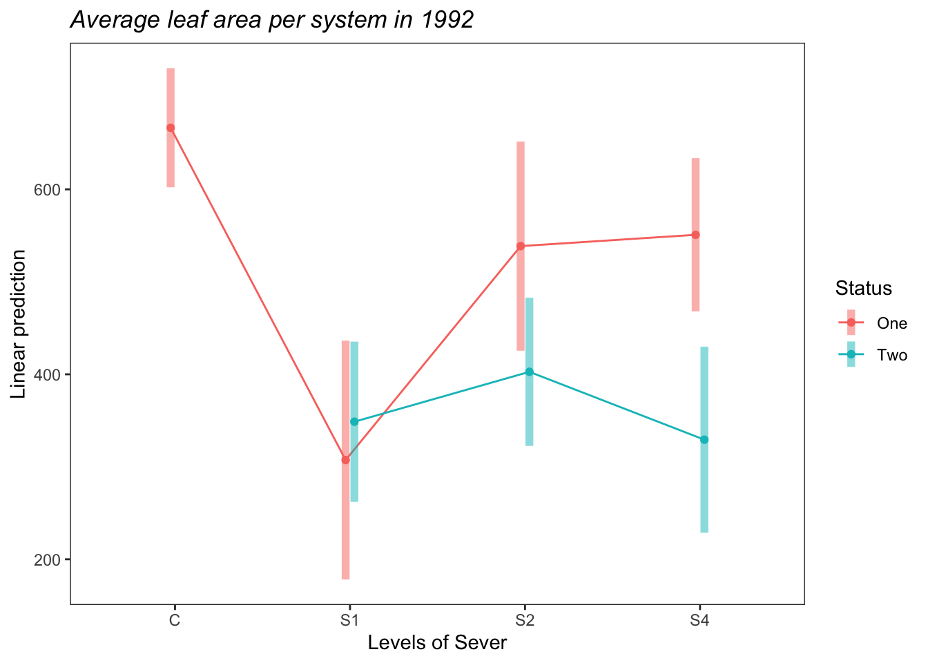
b<-emmip(s92mod2, Sever~Status  ,CIs = TRUE)+ ggtitle("Average leaf area per system in 1992")+
  theme_bw()+theme(plot.title = element_text(face="italic"))+theme(panel.grid.major = element_blank(), panel.grid.minor = element_blank())

b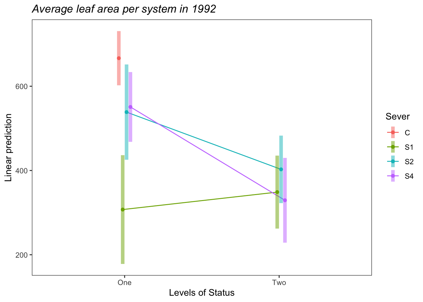
9.5 Manuscript plots with 0-1-2
For 1991, the leaf area in each year, with the total leaf area as an inset:
s91mod1<-lmer(Lftot_91~Status*Sever+(1|COLONY), data = mayappleData91)
a<-emmip(s91mod1, Sever~Status  ,CIs = TRUE)+ ylab("Total leaf area")+
  theme_bw()+theme(panel.grid.major = element_blank(), panel.grid.minor = element_blank())+xlab("")+theme(legend.position = "none")+theme(panel.border = element_blank(), axis.line = element_line())

counts<-mayappleData91 %>% group_by(Status, Sever) %>%
  count(N=length(Sever))

s91mod2<-lmer(Lf91s~Status*Sever+(1|COLONY), data = mayappleData91)
b<-emmip(s91mod2, Sever~Status  ,CIs = TRUE)+ ylab("Average leaf area per system")+
  theme_bw()+theme(panel.grid.major = element_blank(), panel.grid.minor = element_blank())+scale_y_continuous(limits=c(-250, 1500))+ geom_text(data=counts, aes(x=Status, y=N, label=N, color=Sever))


ggdraw(b) +
  draw_plot(a, .35, .47, .6, .6, scale=0.75)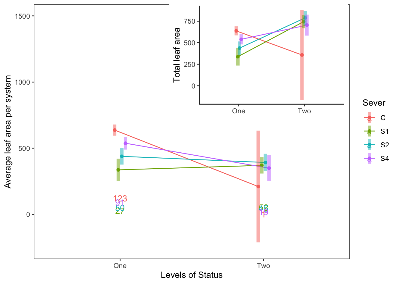
The same thing for 1992:
s92mod1<-lmer(Lftot_92~Status*Sever+(1|COLONY), data = mayappleData92)
a<-emmip(s92mod1, Sever~Status  ,CIs = TRUE)+ ylab("Total leaf area")+
  theme_bw()+theme(panel.grid.major = element_blank(), panel.grid.minor = element_blank())+xlab("")+theme(legend.position = "none")+theme(panel.border = element_blank(), axis.line = element_line())

counts<-mayappleData92 %>% group_by(Status, Sever) %>%
  count(N=length(Sever))

s92mod2<-lmer(Lf92s~Status*Sever+(1|COLONY), data = mayappleData92)
b<-emmip(s92mod2, Sever~Status  ,CIs = TRUE)+ ylab("Average leaf area per system")+
  theme_bw()+theme(panel.grid.major = element_blank(), panel.grid.minor = element_blank())+scale_y_continuous(limits=c(-250, 1500))+ geom_text(data=counts, aes(x=Status, y=N, label=N, color=Sever))

ggdraw(b) +
  draw_plot(a, .35, .47, .6, .6, scale=0.75)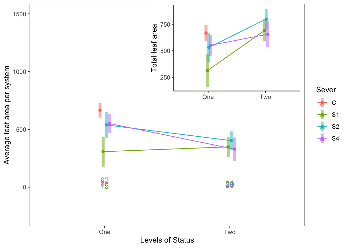
9.6 1991
9.6.1 1991 tables
A table of system status (Front = front system only, Back = back system only, Both = front & back, None = dead (no front, no back)) first in total, and then across the treatments:
mayappleData91 %>% mutate(Status = case_when(LfFtot_91!=0 & LfBtot_91!=0 ~"Both",
                                             LfFtot_91==0 & LfBtot_91!=0 ~"Back",
                                             LfFtot_91!=0 & LfBtot_91==0 ~"Front",
                                             LfFtot_91==0 & LfBtot_91==0 ~"None")) %>%
  group_by(Status) %>%
  summarise(N=length(Sever)) %>%
kable()| Status | N |
|---|---|
| Back | 15 |
| Both | 117 |
| Front | 276 |
Summary: Most systems have only a front system. Having only a back system is rare across all treatments.
mayappleData91 %>% mutate(Status = case_when(LfFtot_91!=0 & LfBtot_91!=0 ~"Both",
                                             LfFtot_91==0 & LfBtot_91!=0 ~"Back",
                                             LfFtot_91!=0 & LfBtot_91==0 ~"Front",
                                             LfFtot_91==0 & LfBtot_91==0 ~"None")) %>%
  group_by(Sever,Status) %>%
  summarise(N=length(Sever)) %>%
kable()| Sever | Status | N |
|---|---|---|
| C | Both | 1 |
| C | Front | 123 |
| S1 | Back | 7 |
| S1 | Both | 52 |
| S1 | Front | 20 |
| S2 | Back | 6 |
| S2 | Both | 45 |
| S2 | Front | 44 |
| S4 | Back | 2 |
| S4 | Both | 19 |
| S4 | Front | 89 |
Summary: Almost all control systems have front systems only. The majority of S1 systems have both systems. S2 systems are equally likely to have a front system or both systems. Most S4 systems only have a front system. Across the severing treatments, there were between 7 and 15 systems that were dead (e.g. zero front and zero back).
9.6.2 1991 contingency table analysis:
mayappleData91 <- mayappleData91 %>% mutate(Status = case_when(LfFtot_91!=0 & LfBtot_91!=0 ~"Both",
                                             LfFtot_91==0 & LfBtot_91!=0 ~"Back",
                                             LfFtot_91!=0 & LfBtot_91==0 ~"Front",
                                             LfFtot_91==0 & LfBtot_91==0 ~"None")) %>%
  mutate(Status = factor(Status, levels=c("None", "Front", "Back", "Both")))

chisq.test(mayappleData91$Status, mayappleData91$Sever)
##
## Pearson's Chi-squared test
##
## data: mayappleData91$Status and mayappleData91$Sever
## X-squared = 149.75, df = 6, p-value < 2.2e-16## mayappleData91$Sever
## mayappleData91$Status C S1 S2 S4
## Front 123 20 44 89
## Back 0 7 6 2
## Both 1 52 45 19## mayappleData91$Sever
## mayappleData91$Status C S1 S2 S4
## Front 83.882353 53.441176 64.264706 74.411765
## Back 4.558824 2.904412 3.492647 4.044118
## Both 35.558824 22.654412 27.242647 31.544118## mayappleData91$Sever
## mayappleData91$Status C S1 S2 S4
## Front 4.271077 -4.574499 -2.527866 1.691149
## Back -2.135140 2.403185 1.341647 -1.016469
## Both -5.795425 6.165473 3.402151 -2.2334749.6.3 1991 total leaf area analysis
Note: This is somewhat challenging, because we don’t have any back-only controls, and we have just one control with both systems.
mayappleData91 <- mayappleData91 %>% mutate(Status = case_when(LfFtot_91!=0 & LfBtot_91!=0 ~"Both",
                                             LfFtot_91==0 & LfBtot_91!=0 ~"Back",
                                             LfFtot_91!=0 & LfBtot_91==0 ~"Front",
                                             LfFtot_91==0 & LfBtot_91==0 ~"None")) %>%
  mutate(Status = factor(Status, levels=c("None", "Front", "Back", "Both"))) %>%
  filter(Status != "None")

s91mod1<-lmer(Lftot_91~Status*Sever+(1|COLONY), data = mayappleData91)
anova(s91mod1)
## Type III Analysis of Variance Table with Satterthwaite's method
## Sum Sq Mean Sq NumDF DenDF F value Pr(>F)
## Status 981778 490889 2 391.41 7.3160 0.0007597 ***
## Sever 88826 29609 3 387.99 0.4413 0.7236156
## Status:Sever 1194568 238914 5 391.32 3.5606 0.0036793 **
## ---
## Signif. codes: 0 '***' 0.001 '**' 0.01 '*' 0.05 '.' 0.1 ' ' 1## $emmeans
## Status emmean SE df lower.CL upper.CL
## Front 481 23.3 81 434 527
## Back nonEst NA NA NA NA
## Both 645 69.8 393 508 783
##
## Results are averaged over the levels of: Sever
## Degrees-of-freedom method: satterthwaite
## Confidence level used: 0.95
##
## $contrasts
## contrast estimate SE df t.ratio p.value
## Front - Back nonEst NA NA NA NA
## Front - Both -165 71.5 389 -2.302 0.0567
## Back - Both nonEst NA NA NA NA
##
## Results are averaged over the levels of: Sever
## Degrees-of-freedom method: satterthwaite
## P value adjustment: tukey method for comparing a family of 3 estimates## $emmeans
## Status = Front:
## Sever emmean SE df lower.CL upper.CL
## C 637 26.3 131 585 689
## S1 294 60.8 364 175 414
## S2 445 41.2 317 364 526
## S4 547 30.1 186 487 606
##
## Status = Back:
## Sever emmean SE df lower.CL upper.CL
## C nonEst NA NA NA NA
## S1 451 100.4 397 254 648
## S2 380 108.4 397 166 593
## S4 189 186.3 393 -178 555
##
## Status = Both:
## Sever emmean SE df lower.CL upper.CL
## C 345 263.4 392 -173 863
## S1 744 38.6 269 668 820
## S2 788 41.1 298 708 869
## S4 704 61.6 383 583 825
##
## Degrees-of-freedom method: satterthwaite
## Confidence level used: 0.95
##
## $contrasts
## Status = Front:
## contrast estimate SE df t.ratio p.value
## C - S1 342.8 63.9 396 5.362 <.0001
## C - S2 191.8 46.0 388 4.168 0.0002
## C - S4 90.3 36.3 382 2.487 0.0636
## S1 - S2 -150.9 71.5 396 -2.111 0.1512
## S1 - S4 -252.5 65.8 397 -3.839 0.0008
## S2 - S4 -101.6 48.2 386 -2.107 0.1527
##
## Status = Back:
## contrast estimate SE df t.ratio p.value
## C - S1 nonEst NA NA NA NA
## C - S2 nonEst NA NA NA NA
## C - S4 nonEst NA NA NA NA
## S1 - S2 71.3 146.5 392 0.487 0.9620
## S1 - S4 262.3 210.5 389 1.246 0.5980
## S2 - S4 191.0 214.4 389 0.891 0.8095
##
## Status = Both:
## contrast estimate SE df t.ratio p.value
## C - S1 -398.7 265.8 391 -1.500 0.4385
## C - S2 -443.1 266.3 392 -1.664 0.3443
## C - S4 -358.7 270.3 392 -1.327 0.5461
## S1 - S2 -44.5 53.3 388 -0.834 0.8384
## S1 - S4 40.0 69.9 382 0.572 0.9405
## S2 - S4 84.4 71.6 386 1.179 0.6403
##
## Degrees-of-freedom method: satterthwaite
## P value adjustment: tukey method for comparing a family of 4 estimatesemmip(s91mod1, Status~Sever,CIs = TRUE)+ ggtitle("Total leaf area in 1991")+
theme_bw()+theme(plot.title = element_text(face="italic"))+theme(panel.grid.major = element_blank(), panel.grid.minor = element_blank())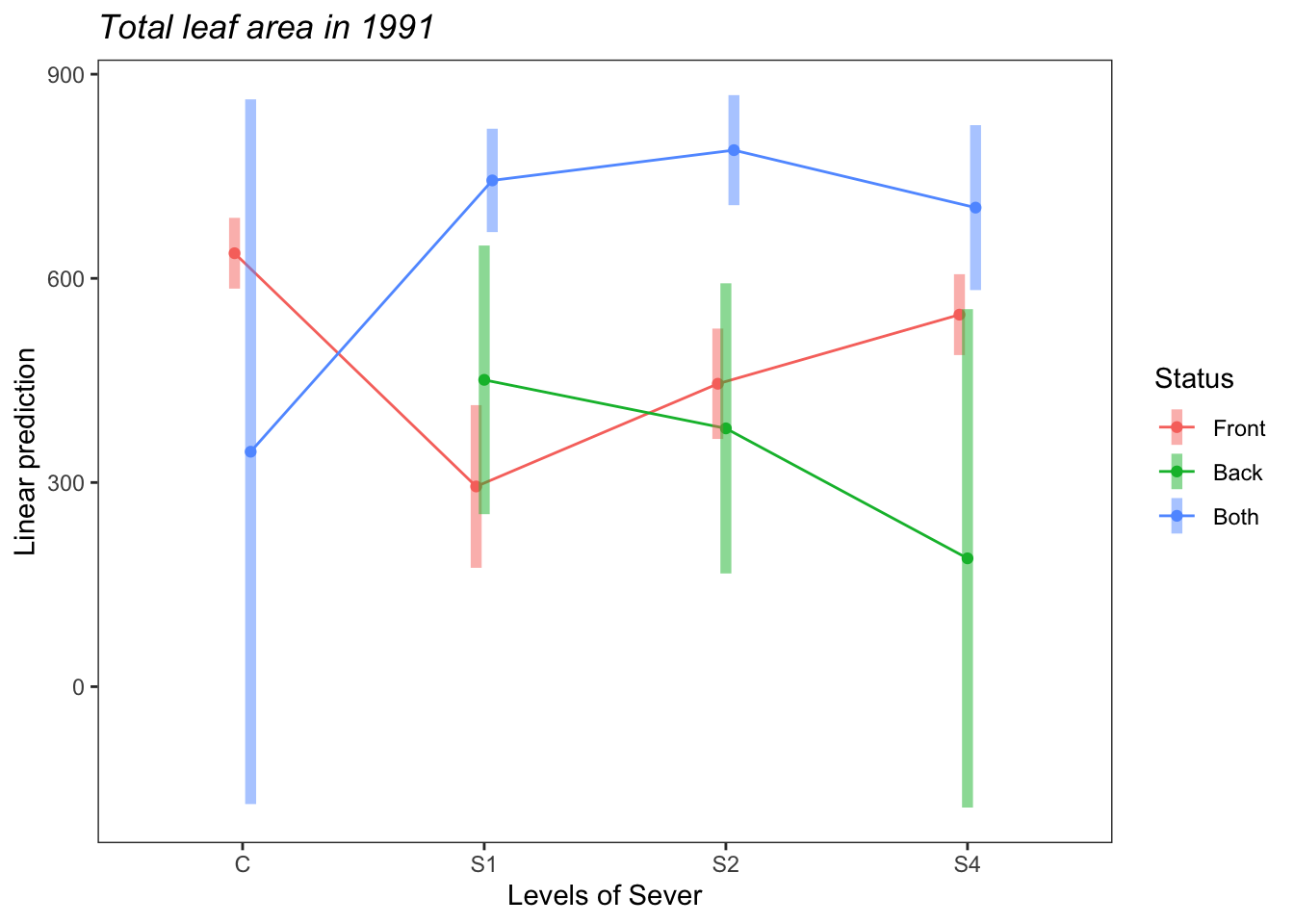
a<-emmip(s91mod1, Sever~Status  ,CIs = TRUE)+ ggtitle("Total leaf area in 1991")+
  theme_bw()+theme(plot.title = element_text(face="italic"))+theme(panel.grid.major = element_blank(), panel.grid.minor = element_blank())

a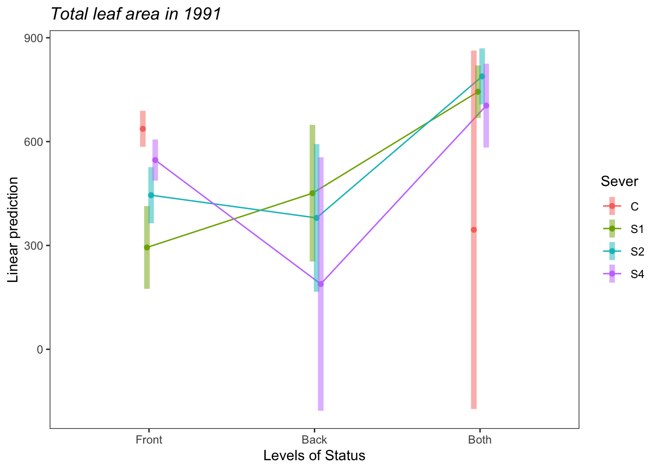
Both systems have marginally more leaf area than Front systems.
9.6.4 1991 leaf area analysis per system
mayappleData91 <- mayappleData91 %>% mutate(Lf91s=ifelse(Status=="Both", Lftot_91/2, Lftot_91))


s91mod2<-lmer(Lf91s~Status*Sever+(1|COLONY), data = mayappleData91)
anova(s91mod2)
## Type III Analysis of Variance Table with Satterthwaite's method
## Sum Sq Mean Sq NumDF DenDF F value Pr(>F)
## Status 339007 169503 2 391.75 3.8475 0.022144 *
## Sever 41595 13865 3 388.44 0.3147 0.814745
## Status:Sever 897745 179549 5 391.72 4.0755 0.001282 **
## ---
## Signif. codes: 0 '***' 0.001 '**' 0.01 '*' 0.05 '.' 0.1 ' ' 1## $emmeans
## Status emmean SE df lower.CL upper.CL
## Front 480 18.7 82.9 443 517
## Back nonEst NA NA NA NA
## Both 328 56.5 393.1 217 439
##
## Results are averaged over the levels of: Sever
## Degrees-of-freedom method: satterthwaite
## Confidence level used: 0.95
##
## $contrasts
## contrast estimate SE df t.ratio p.value
## Front - Back nonEst NA NA NA NA
## Front - Both 152 57.9 390 2.627 0.0243
## Back - Both nonEst NA NA NA NA
##
## Results are averaged over the levels of: Sever
## Degrees-of-freedom method: satterthwaite
## P value adjustment: tukey method for comparing a family of 3 estimates## $emmeans
## Status = Front:
## Sever emmean SE df lower.CL upper.CL
## C 637 21.2 135 595 679
## S1 292 49.1 365 195 388
## S2 445 33.3 320 380 511
## S4 545 24.3 191 497 593
##
## Status = Back:
## Sever emmean SE df lower.CL upper.CL
## C nonEst NA NA NA NA
## S1 451 81.3 397 291 611
## S2 386 87.8 397 213 558
## S4 180 150.8 393 -117 476
##
## Status = Both:
## Sever emmean SE df lower.CL upper.CL
## C 198 213.3 393 -221 618
## S1 371 31.1 273 309 432
## S2 392 33.2 301 327 457
## S4 349 49.9 384 251 447
##
## Degrees-of-freedom method: satterthwaite
## Confidence level used: 0.95
##
## $contrasts
## Status = Front:
## contrast estimate SE df t.ratio p.value
## C - S1 345.1 51.8 396 6.669 <.0001
## C - S2 191.3 37.3 388 5.132 <.0001
## C - S4 91.5 29.4 383 3.113 0.0107
## S1 - S2 -153.8 57.9 396 -2.658 0.0406
## S1 - S4 -253.6 53.2 397 -4.763 <.0001
## S2 - S4 -99.8 39.0 387 -2.555 0.0534
##
## Status = Back:
## contrast estimate SE df t.ratio p.value
## C - S1 nonEst NA NA NA NA
## C - S2 nonEst NA NA NA NA
## C - S4 nonEst NA NA NA NA
## S1 - S2 65.7 118.7 393 0.553 0.9456
## S1 - S4 271.3 170.5 390 1.591 0.3848
## S2 - S4 205.7 173.6 389 1.185 0.6369
##
## Status = Both:
## contrast estimate SE df t.ratio p.value
## C - S1 -172.3 215.3 392 -0.800 0.8542
## C - S2 -193.5 215.7 392 -0.897 0.8062
## C - S4 -151.1 218.9 392 -0.690 0.9007
## S1 - S2 -21.3 43.2 388 -0.492 0.9608
## S1 - S4 21.2 56.6 383 0.374 0.9822
## S2 - S4 42.4 58.0 386 0.732 0.8844
##
## Degrees-of-freedom method: satterthwaite
## P value adjustment: tukey method for comparing a family of 4 estimates## $emmeans
## Sever = C:
## Status emmean SE df lower.CL upper.CL
## Front 637 21.2 135 595 679
## Back nonEst NA NA NA NA
## Both 198 213.3 393 -221 618
##
## Sever = S1:
## Status emmean SE df lower.CL upper.CL
## Front 292 49.1 365 195 388
## Back 451 81.3 397 291 611
## Both 371 31.1 273 309 432
##
## Sever = S2:
## Status emmean SE df lower.CL upper.CL
## Front 445 33.3 320 380 511
## Back 386 87.8 397 213 558
## Both 392 33.2 301 327 457
##
## Sever = S4:
## Status emmean SE df lower.CL upper.CL
## Front 545 24.3 191 497 593
## Back 180 150.8 393 -117 476
## Both 349 49.9 384 251 447
##
## Degrees-of-freedom method: satterthwaite
## Confidence level used: 0.95
##
## $contrasts
## Sever = C:
## contrast estimate SE df t.ratio p.value
## Front - Back nonEst NA NA NA NA
## Front - Both 438.38 214.0 392 2.049 0.1022
## Back - Both nonEst NA NA NA NA
##
## Sever = S1:
## contrast estimate SE df t.ratio p.value
## Front - Back -159.61 94.3 396 -1.693 0.2090
## Front - Both -79.02 56.9 397 -1.390 0.3473
## Back - Both 80.59 86.2 396 0.935 0.6186
##
## Sever = S2:
## contrast estimate SE df t.ratio p.value
## Front - Back 59.88 93.1 395 0.643 0.7962
## Front - Both 53.55 45.4 396 1.180 0.4661
## Back - Both -6.34 93.2 396 -0.068 0.9975
##
## Sever = S4:
## contrast estimate SE df t.ratio p.value
## Front - Back 365.33 152.2 390 2.400 0.0444
## Front - Both 195.74 54.0 394 3.625 0.0010
## Back - Both -169.58 158.6 392 -1.069 0.5338
##
## Degrees-of-freedom method: satterthwaite
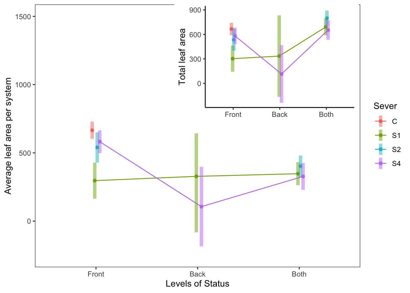
## P value adjustment: tukey method for comparing a family of 3 estimatesemmip(s91mod2, Status~Sever,CIs = TRUE)+ ggtitle("Average leaf area per system in 1991")+
theme_bw()+theme(plot.title = element_text(face="italic"))+theme(panel.grid.major = element_blank(), panel.grid.minor = element_blank())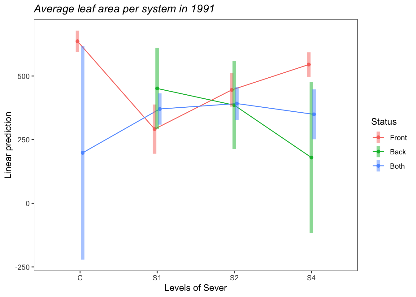
b<-emmip(s91mod2, Sever~Status  ,CIs = TRUE)+ ggtitle("Average leaf area per system in 1991")+
  theme_bw()+theme(plot.title = element_text(face="italic"))+theme(panel.grid.major = element_blank(), panel.grid.minor = element_blank())

b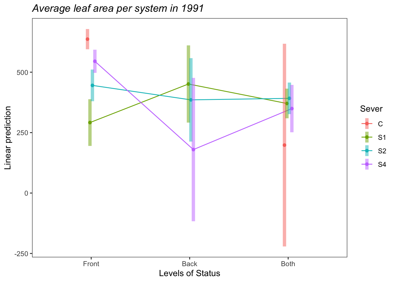
So the average leaf area per system of Front systems is greater than the average leaf area per system of Both systems. This is probably driven by the higher leaf area of Front systems in the Control treatment.
9.7 1992
9.7.1 1992 tables
A table of system status (Front = front system only, Back = back system only, Both = front & back, None = dead (zero front, zero back)) first in total, and then across the treatments:
mayappleData92 %>% mutate(Status = case_when(LftotF_92!=0 & LftotB_92!=0 ~"Both",
                                             LftotF_92==0 & LftotB_92!=0 ~"Back",
                                             LftotF_92!=0 & LftotB_92==0 ~"Front",
                                             LftotF_92==0 & LftotB_92==0 ~"None")) %>%
  group_by(Status) %>%
  summarise(N=length(Sever)) %>%
kable()| Status | N |
|---|---|
| Back | 3 |
| Both | 83 |
| Front | 117 |
mayappleData92 %>% mutate(Status = case_when(LftotF_92!=0 & LftotB_92!=0 ~"Both",
                                             LftotF_92==0 & LftotB_92!=0 ~"Back",
                                             LftotF_92!=0 & LftotB_92==0 ~"Front",
                                             LftotF_92==0 & LftotB_92==0 ~"None")) %>%
  group_by(Sever,Status) %>%
  summarise(N=length(Sever)) %>%
kable()| Sever | Status | N |
|---|---|---|
| C | Front | 62 |
| S1 | Back | 1 |
| S1 | Both | 29 |
| S1 | Front | 11 |
| S2 | Both | 34 |
| S2 | Front | 15 |
| S4 | Back | 2 |
| S4 | Both | 20 |
| S4 | Front | 29 |
Summary: Control systems have front systems only (or no system). Having only a back system is rare across all treatments (N=3 total across the treatments). The majority of S1 systems have both systems. The majority of S2 systems have both systems. S4 systems are about equally likely to have a front system or both systems. Across the treatments, the number of dead (None) systems is relatively low and consistent (between 1 and 8 systems).
9.7.2 1992 contingency table analysis:
mayappleData92 <- mayappleData92 %>% mutate(Status = case_when(LftotF_92!=0 & LftotB_92!=0 ~"Both",
                                             LftotF_92==0 & LftotB_92!=0 ~"Back",
                                             LftotF_92!=0 & LftotB_92==0 ~"Front",
                                             LftotF_92==0 & LftotB_92==0 ~"None")) %>%
  mutate(Status = factor(Status, levels=c("None", "Front", "Back", "Both")))

chisq.test(mayappleData92$Status, mayappleData92$Sever)
##
## Pearson's Chi-squared test
##
## data: mayappleData92$Status and mayappleData92$Sever
## X-squared = 80.28, df = 6, p-value = 3.127e-15## mayappleData92$Sever
## mayappleData92$Status C S1 S2 S4
## Front 62 11 15 29
## Back 0 1 0 2
## Both 0 29 34 20## mayappleData92$Sever
## mayappleData92$Status C S1 S2 S4
## Front 35.7339901 23.6305419 28.2413793 29.3940887
## Back 0.9162562 0.6059113 0.7241379 0.7536946
## Both 25.3497537 16.7635468 20.0344828 20.8522167## mayappleData92$Sever
## mayappleData92$Status C S1 S2 S4
## Front 4.39393215 -2.59827517 -2.49166857 -0.07268821
## Back -0.95721270 0.50627842 -0.85096294 1.43557798
## Both -5.03485389 2.98863307 3.12009601 -0.186626779.7.3 1992 total leaf area analysis
Note: Again, this is somewhat challenging, because of the very small number of back-only systems. Also there were no controls with both systems, and the number of None systems is very low in each severing treatment.
mayappleData92 <- mayappleData92 %>% mutate(Status = case_when(LftotF_92!=0 & LftotB_92!=0 ~"Both",
                                             LftotF_92==0 & LftotB_92!=0 ~"Back",
                                             LftotF_92!=0 & LftotB_92==0 ~"Front",
                                             LftotF_92==0 & LftotB_92==0 ~"None")) %>%
  mutate(Status = factor(Status, levels=c("None", "Front", "Back", "Both"))) %>%
  filter(Status != "None")


s92mod<-lmer(Lftot_92~Status*Sever+(1|COLONY), data = mayappleData92)
anova(s92mod)
## Type III Analysis of Variance Table with Satterthwaite's method
## Sum Sq Mean Sq NumDF DenDF F value Pr(>F)
## Status 1906748 953374 2 190.03 15.4428 6.104e-07 ***
## Sever 1294318 431439 3 188.38 6.9885 0.0001754 ***
## Status:Sever 536345 178782 3 191.07 2.8959 0.0364339 *
## ---
## Signif. codes: 0 '***' 0.001 '**' 0.01 '*' 0.05 '.' 0.1 ' ' 1## $emmeans
## Status emmean SE df lower.CL upper.CL
## Front 521 35.3 36.6 450 593
## Back nonEst NA NA NA NA
## Both nonEst NA NA NA NA
##
## Results are averaged over the levels of: Sever
## Degrees-of-freedom method: satterthwaite
## Confidence level used: 0.95
##
## $contrasts
## contrast estimate SE df z.ratio p.value
## Front - Back nonEst NA NA NA NA
## Front - Both nonEst NA NA NA NA
## Back - Both nonEst NA NA NA NA
##
## Results are averaged over the levels of: Sever
## Degrees-of-freedom method: satterthwaite
## P value adjustment: tukey method for comparing a family of 3 estimates## $emmeans
## Sever = C:
## Status emmean SE df lower.CL upper.CL
## Front 667 37.6 48.5 591 742
## Back nonEst NA NA NA NA
## Both nonEst NA NA NA NA
##
## Sever = S1:
## Status emmean SE df lower.CL upper.CL
## Front 302 81.1 159.8 142 463
## Back 334 253.2 189.8 -166 833
## Both 691 51.7 101.7 589 794
##
## Sever = S2:
## Status emmean SE df lower.CL upper.CL
## Front 534 68.1 165.8 399 668
## Back nonEst NA NA NA NA
## Both 798 47.7 92.2 703 893
##
## Sever = S4:
## Status emmean SE df lower.CL upper.CL
## Front 582 50.8 110.0 481 683
## Back 115 179.7 192.4 -240 469
## Both 654 60.4 138.2 534 773
##
## Degrees-of-freedom method: satterthwaite
## Confidence level used: 0.95
##
## $contrasts
## Sever = C:
## contrast estimate SE df t.ratio p.value
## Front - Back nonEst NA NA NA NA
## Front - Both nonEst NA NA NA NA
## Back - Both nonEst NA NA NA NA
##
## Sever = S1:
## contrast estimate SE df t.ratio p.value
## Front - Back -31.6 264.2 188 -0.120 0.9921
## Front - Both -388.9 92.4 193 -4.211 0.0001
## Back - Both -357.3 256.4 187 -1.393 0.3464
##
## Sever = S2:
## contrast estimate SE df t.ratio p.value
## Front - Back nonEst NA NA NA NA
## Front - Both -264.2 78.0 187 -3.388 0.0025
## Back - Both nonEst NA NA NA NA
##
## Sever = S4:
## contrast estimate SE df t.ratio p.value
## Front - Back 467.3 184.9 189 2.528 0.0328
## Front - Both -71.7 74.3 192 -0.965 0.5996
## Back - Both -539.0 187.0 187 -2.883 0.0122
##
## Degrees-of-freedom method: satterthwaite
## P value adjustment: tukey method for comparing a family of 3 estimatesemmip(s92mod, ~Status~Sever ,CIs = TRUE)+ ggtitle("Total leaf area in 1992")+
theme_bw()+theme(plot.title = element_text(face="italic"))+theme(panel.grid.major = element_blank(), panel.grid.minor = element_blank())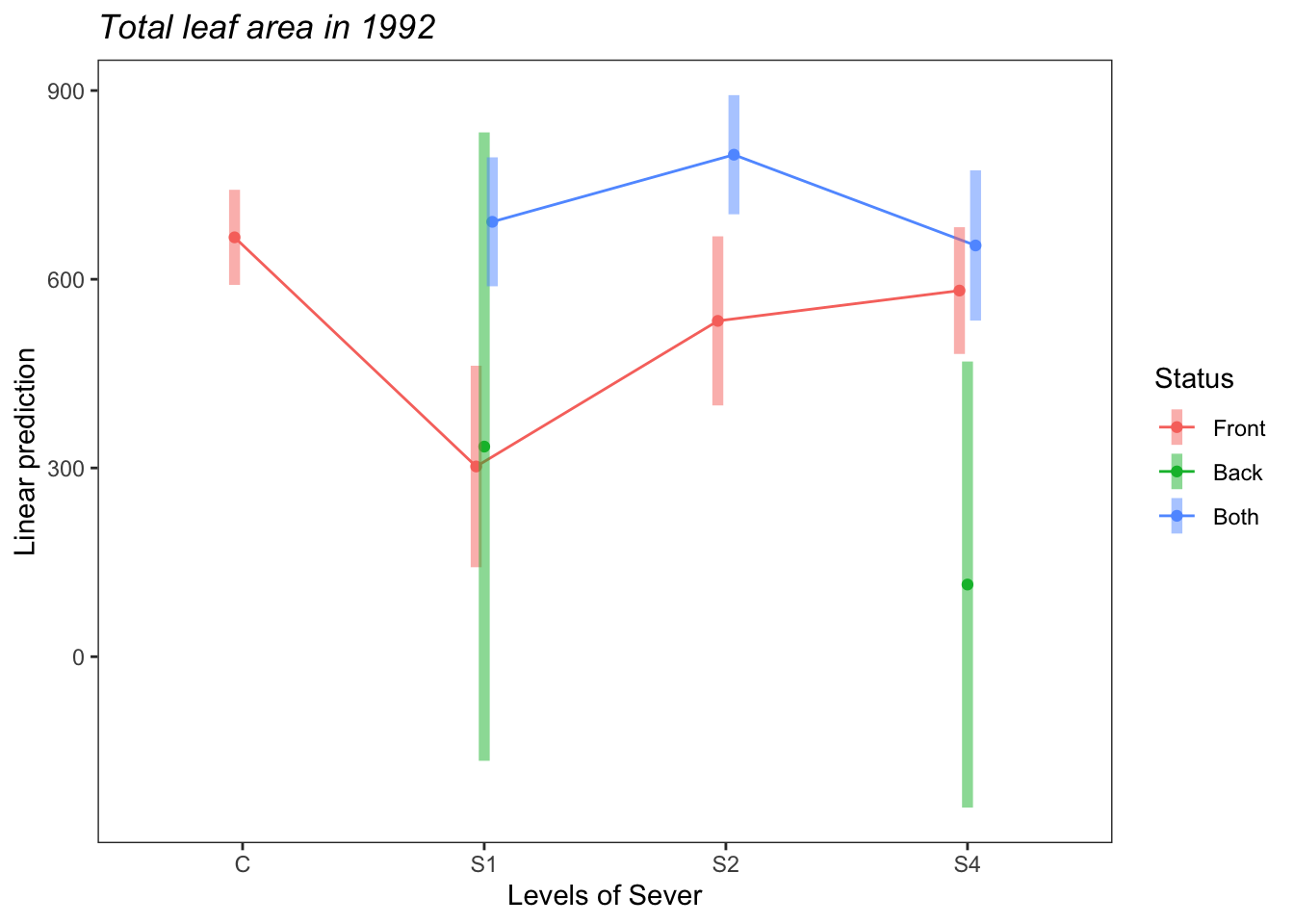
c<-emmip(s92mod, ~Sever~Status  ,CIs = TRUE)+ ggtitle("Total leaf area in 1992")+
  theme_bw()+theme(plot.title = element_text(face="italic"))+theme(panel.grid.major = element_blank(), panel.grid.minor = element_blank())

c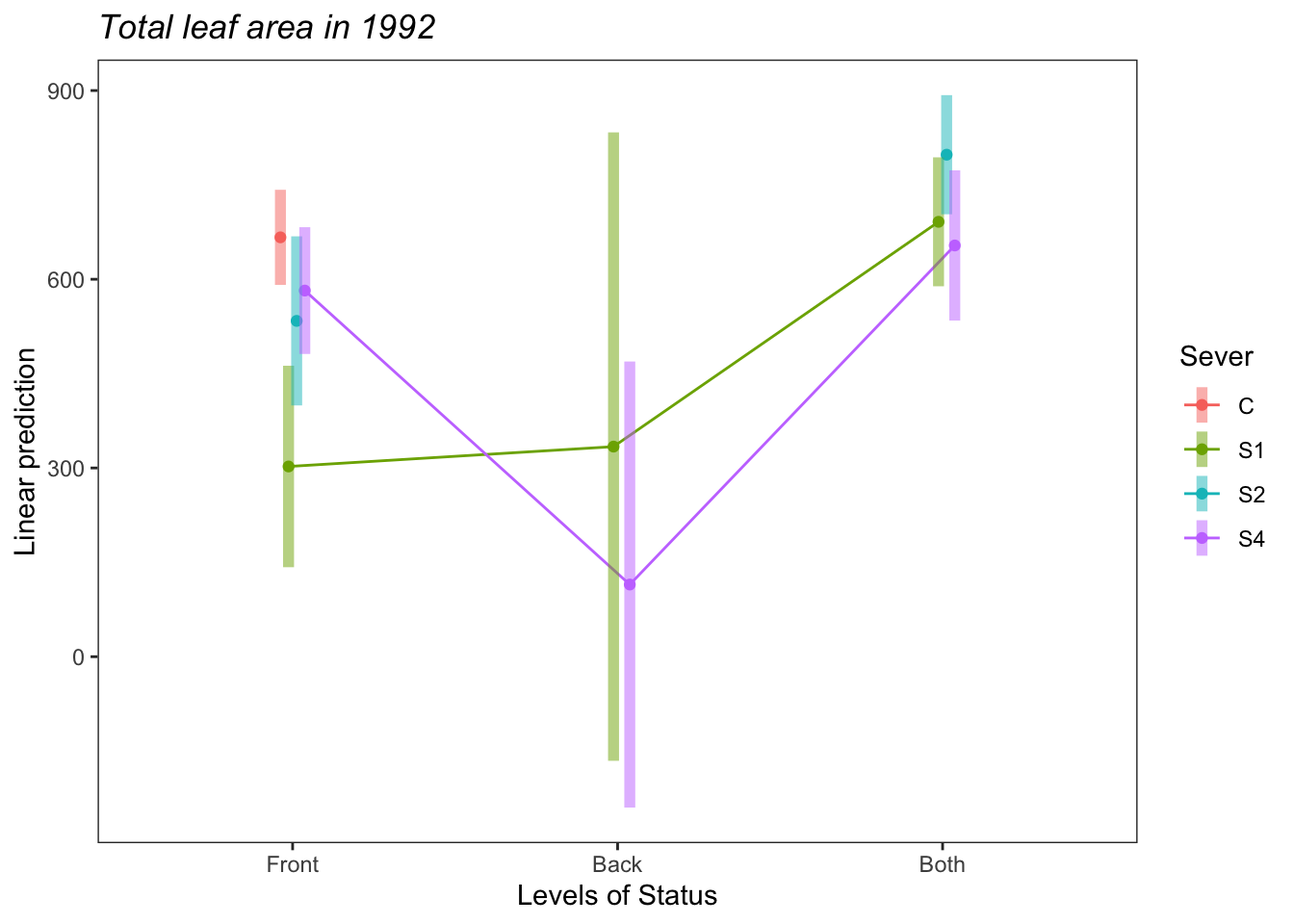
9.7.4 1992 leaf area analysis per system
mayappleData92 <- mayappleData92 %>%
  mutate(Lf92s=ifelse(Status=="Both", Lftot_92/2, Lftot_92))


s92mod<-lmer(Lf92s~Status*Sever+(1|COLONY), data = mayappleData92)
anova(s92mod)
## Type III Analysis of Variance Table with Satterthwaite's method
## Sum Sq Mean Sq NumDF DenDF F value Pr(>F)
## Status 413983 206992 2 189.87 4.9708 0.007867 **
## Sever 1149965 383322 3 188.12 9.2054 1.032e-05 ***
## Status:Sever 474768 158256 3 190.80 3.8005 0.011184 *
## ---
## Signif. codes: 0 '***' 0.001 '**' 0.01 '*' 0.05 '.' 0.1 ' ' 1## $emmeans
## Status emmean SE df lower.CL upper.CL
## Front 521 29.3 35.4 462 580
## Back nonEst NA NA NA NA
## Both nonEst NA NA NA NA
##
## Results are averaged over the levels of: Sever
## Degrees-of-freedom method: satterthwaite
## Confidence level used: 0.95
##
## $contrasts
## contrast estimate SE df z.ratio p.value
## Front - Back nonEst NA NA NA NA
## Front - Both nonEst NA NA NA NA
## Back - Both nonEst NA NA NA NA
##
## Results are averaged over the levels of: Sever
## Degrees-of-freedom method: satterthwaite
## P value adjustment: tukey method for comparing a family of 3 estimates## $emmeans
## Status = Front:
## Sever emmean SE df lower.CL upper.CL
## C 666 31.2 46.7 603.2 729
## S1 297 66.8 158.9 164.7 429
## S2 540 56.1 163.7 429.3 651
## S4 582 42.0 106.7 498.7 665
##
## Status = Back:
## Sever emmean SE df lower.CL upper.CL
## C nonEst NA NA NA NA
## S1 328 208.1 189.7 -82.4 738
## S2 nonEst NA NA NA NA
## S4 106 147.7 192.3 -185.2 398
##
## Status = Both:
## Sever emmean SE df lower.CL upper.CL
## C nonEst NA NA NA NA
## S1 347 42.7 99.0 262.7 432
## S2 402 39.4 89.1 324.1 481
## S4 327 49.8 135.6 229.0 426
##
## Degrees-of-freedom method: satterthwaite
## Confidence level used: 0.95
##
## $contrasts
## Status = Front:
## contrast estimate SE df t.ratio p.value
## C - S1 369.2 69.7 194 5.296 <.0001
## C - S2 125.9 59.6 188 2.113 0.1528
## C - S4 84.0 46.3 185 1.814 0.2701
## S1 - S2 -243.3 83.9 194 -2.898 0.0216
## S1 - S4 -285.2 75.7 194 -3.768 0.0012
## S2 - S4 -41.9 65.9 188 -0.636 0.9204
##
## Status = Back:
## contrast estimate SE df t.ratio p.value
## C - S1 nonEst NA NA NA NA
## C - S2 nonEst NA NA NA NA
## C - S4 nonEst NA NA NA NA
## S1 - S2 nonEst NA NA NA NA
## S1 - S4 221.9 254.3 187 0.872 0.8191
## S2 - S4 nonEst NA NA NA NA
##
## Status = Both:
## contrast estimate SE df t.ratio p.value
## C - S1 nonEst NA NA NA NA
## C - S2 nonEst NA NA NA NA
## C - S4 nonEst NA NA NA NA
## S1 - S2 -55.0 52.1 186 -1.055 0.7173
## S1 - S4 20.0 59.8 184 0.334 0.9871
## S2 - S4 74.9 58.1 185 1.291 0.5700
##
## Degrees-of-freedom method: satterthwaite
## P value adjustment: tukey method for comparing a family of 4 estimates## $emmeans
## Sever = C:
## Status emmean SE df lower.CL upper.CL
## Front 666 31.2 46.7 603.2 729
## Back nonEst NA NA NA NA
## Both nonEst NA NA NA NA
##
## Sever = S1:
## Status emmean SE df lower.CL upper.CL
## Front 297 66.8 158.9 164.7 429
## Back 328 208.1 189.7 -82.4 738
## Both 347 42.7 99.0 262.7 432
##
## Sever = S2:
## Status emmean SE df lower.CL upper.CL
## Front 540 56.1 163.7 429.3 651
## Back nonEst NA NA NA NA
## Both 402 39.4 89.1 324.1 481
##
## Sever = S4:
## Status emmean SE df lower.CL upper.CL
## Front 582 42.0 106.7 498.7 665
## Back 106 147.7 192.3 -185.2 398
## Both 327 49.8 135.6 229.0 426
##
## Degrees-of-freedom method: satterthwaite
## Confidence level used: 0.95
##
## $contrasts
## Sever = C:
## contrast estimate SE df t.ratio p.value
## Front - Back nonEst NA NA NA NA
## Front - Both nonEst NA NA NA NA
## Back - Both nonEst NA NA NA NA
##
## Sever = S1:
## contrast estimate SE df t.ratio p.value
## Front - Back -31.3 217.1 188 -0.144 0.9886
## Front - Both -50.7 76.0 193 -0.667 0.7826
## Back - Both -19.4 210.7 186 -0.092 0.9954
##
## Sever = S2:
## contrast estimate SE df t.ratio p.value
## Front - Back nonEst NA NA NA NA
## Front - Both 137.6 64.1 187 2.148 0.0831
## Back - Both nonEst NA NA NA NA
##
## Sever = S4:
## contrast estimate SE df t.ratio p.value
## Front - Back 475.7 151.9 188 3.132 0.0057
## Front - Both 254.4 61.1 192 4.167 0.0001
## Back - Both -221.3 153.6 187 -1.440 0.3224
##
## Degrees-of-freedom method: satterthwaite
## P value adjustment: tukey method for comparing a family of 3 estimatesemmip(s92mod, Status~Sever,CIs = TRUE)+ ggtitle("Average leaf area per system in 1992")+
theme_bw()+theme(plot.title = element_text(face="italic"))+theme(panel.grid.major = element_blank(), panel.grid.minor = element_blank())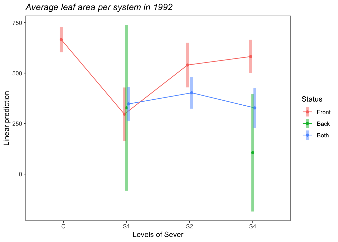
d<-emmip(s92mod, Sever~Status  ,CIs = TRUE)+ ggtitle("Average leaf area per system in 1992")+
  theme_bw()+theme(plot.title = element_text(face="italic"))+theme(panel.grid.major = element_blank(), panel.grid.minor = element_blank())

d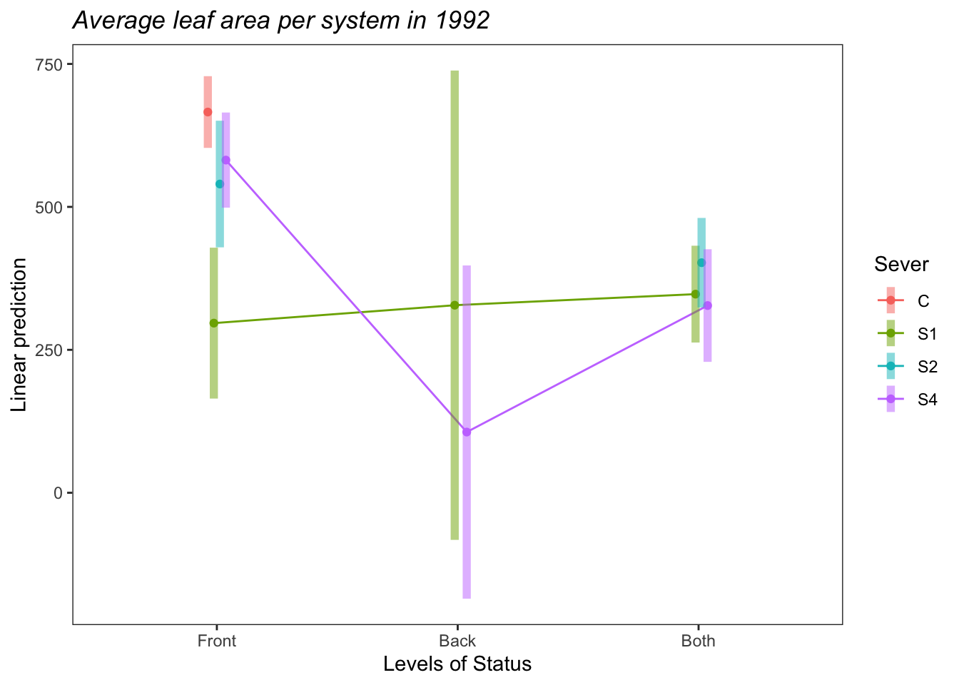
9.7.5 Potential plots for manuscript
Four panel, total and average leaf area in both years:
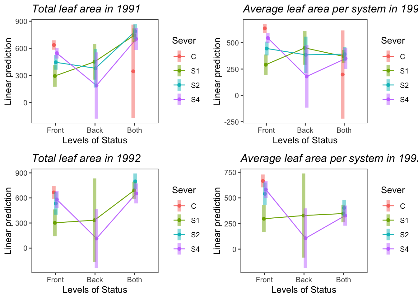
(This can be further cleaned up to only have one legend, etc.)
For 1991, the leaf area in each year, with the total leaf area as an inset:
s91mod1<-lmer(Lftot_91~Status*Sever+(1|COLONY), data = mayappleData91)
a<-emmip(s91mod1, Sever~Status  ,CIs = TRUE)+ ylab("Total leaf area")+
  theme_bw()+theme(panel.grid.major = element_blank(), panel.grid.minor = element_blank())+xlab("")+theme(legend.position = "none")+theme(panel.border = element_blank(), axis.line = element_line())

counts<-mayappleData91 %>% group_by(Status, Sever) %>%
  count(N=length(Sever))

s91mod2<-lmer(Lf91s~Status*Sever+(1|COLONY), data = mayappleData91)
b<-emmip(s91mod2, Sever~Status  ,CIs = TRUE)+ ylab("Average leaf area per system")+
  theme_bw()+theme(panel.grid.major = element_blank(), panel.grid.minor = element_blank())+scale_y_continuous(limits=c(-250, 1500))+ geom_text(data=counts, aes(x=Status, y=N, label=N, color=Sever))


ggdraw(b) +
  draw_plot(a, .35, .47, .6, .6, scale=0.75)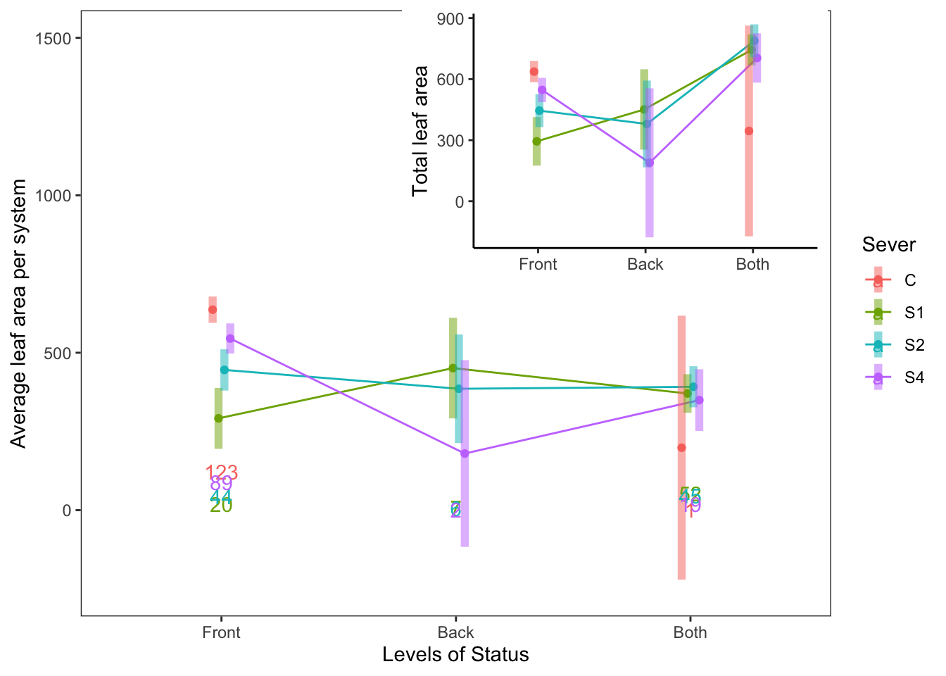
This isn’t perfect, but if we like this idea, I can clean up the plot further (e.g. make the inset plot fit perfectly within the box bounding the larger plot).
For 1991, tri-panel figure with average leaf area, total leaf area, and bar plots.
#a is total leaf area, #b is average leaf area

s91mod1<-lmer(Lftot_91~Status*Sever+(1|COLONY), data = mayappleData91)
## fixed-effect model matrix is rank deficient so dropping 1 column / coefficienta<-emmip(s91mod1, Sever~Status ,CIs = TRUE)+ ylab("Total leaf area")+
theme_bw()+theme(panel.grid.major = element_blank(), panel.grid.minor = element_blank())+xlab("")+theme(legend.position = "none")+xlab("")## Cannot use mode = "kenward-roger" because *pbkrtest* package is not installed## fixed-effect model matrix is rank deficient so dropping 1 column / coefficientb<-emmip(s91mod2, Sever~Status ,CIs = TRUE)+ ylab("Average leaf area per system")+
theme_bw()+theme(panel.grid.major = element_blank(), panel.grid.minor = element_blank())+scale_y_continuous(limits=c(-250, 1500))+xlab("")## Cannot use mode = "kenward-roger" because *pbkrtest* package is not installedcounts<-mayappleData91 %>% group_by(Status, Sever) %>%
count(N=length(Sever))
c<-ggplot(aes(x=Status, y=N, fill=Sever), data=counts)+geom_col(position = "dodge", color="black") +
theme_bw()+theme(panel.grid.major = element_blank(), panel.grid.minor = element_blank()) + geom_text(aes(label=N, color=Sever), position=position_dodge(width=0.9), vjust=-0.25) + ylab("Number of systems")+scale_y_continuous(limits=c(0, 130), breaks=c(0, 50, 100))
library(lemon)##
## Attaching package: 'lemon'## The following object is masked from 'package:purrr':
##
## %||%## The following objects are masked from 'package:ggplot2':
##
## CoordCartesian, element_render## Warning: Removed 1 rows containing missing values (geom_point).## Warning: Removed 1 rows containing missing values (geom_segment).## Warning: Removed 1 rows containing missing values (geom_point).## Warning: Removed 1 rows containing missing values (geom_segment).## Warning: Removed 1 rows containing missing values (geom_point).## Warning: Removed 1 rows containing missing values (geom_segment).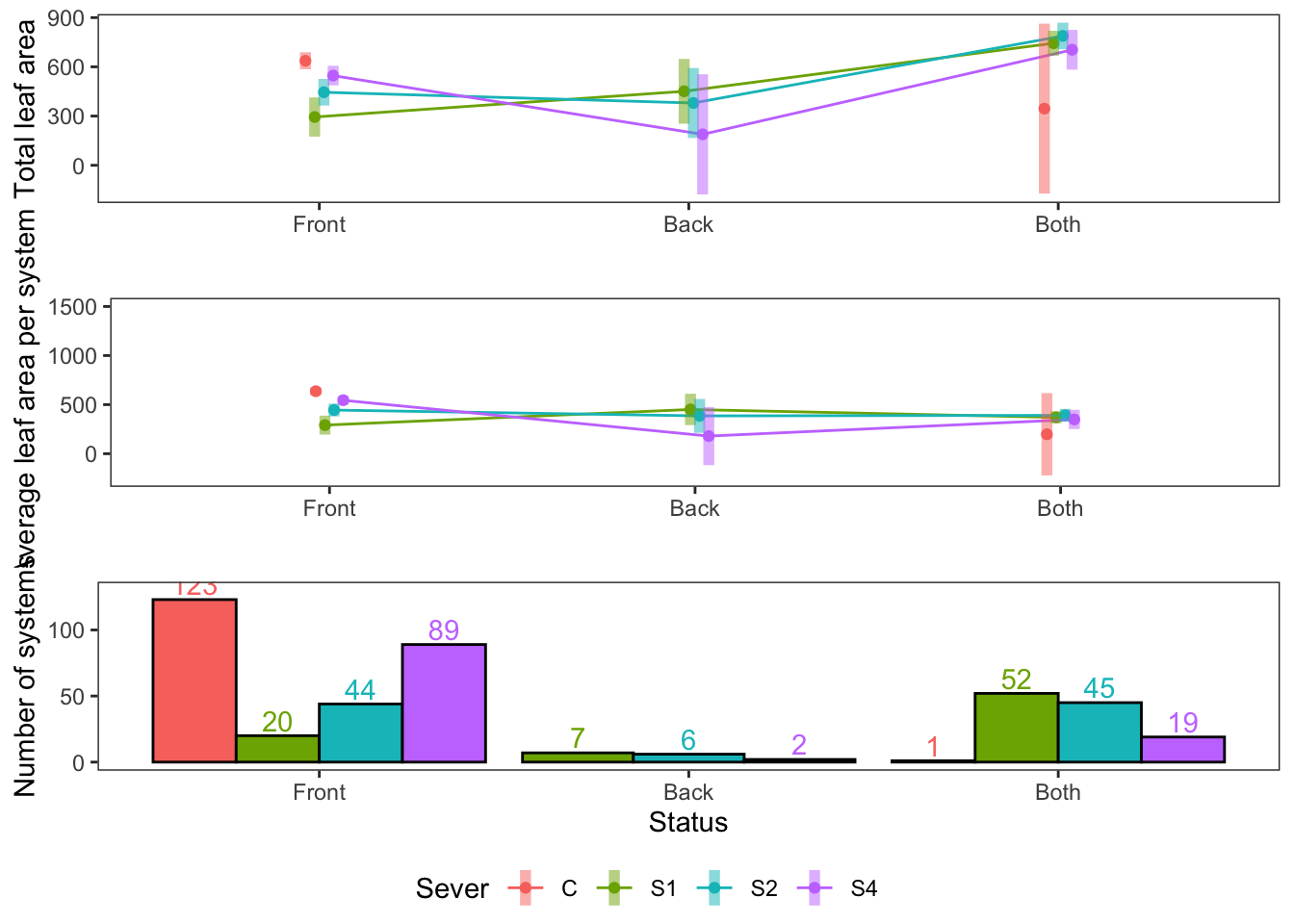
The same thing for 1992:
s92mod1<-lmer(Lftot_92~Status*Sever+(1|COLONY), data = mayappleData92)
a<-emmip(s92mod1, Sever~Status  ,CIs = TRUE)+ ylab("Total leaf area")+
  theme_bw()+theme(panel.grid.major = element_blank(), panel.grid.minor = element_blank())+xlab("")+theme(legend.position = "none")+theme(panel.border = element_blank(), axis.line = element_line())

s92mod2<-lmer(Lf92s~Status*Sever+(1|COLONY), data = mayappleData92)
b<-emmip(s92mod2, Sever~Status  ,CIs = TRUE)+ ylab("Average leaf area per system")+
  theme_bw()+theme(panel.grid.major = element_blank(), panel.grid.minor = element_blank())+scale_y_continuous(limits=c(-250, 1500))

ggdraw(b) +
  draw_plot(a, .35, .47, .6, .6, scale=0.75)