4 1991 back shoot analyses
4.1 Back shoot production
This analysis uses all systems observed in 1991.
4.1.1 Data & visualization
Read in data
# set na.strings="." to recode '.' to NA
mayappleDatasetFull<-readxl::read_excel("Datasets/mayapple_1990_updated.xlsx", na=".")
Select variables from the back of the system. Also filtering out rows that don’t have a leaf area record in 1990. We need to do this in order to be able to compare models from model set A (which don’t include leaf area, and so wouldn’t naturally be affected by the missing data) with models from model set B (which do include leaf area and would be affected by the missing data). In other words, removing these rows means that model set A and model set B will run using the exact same dataset, which is necessary in order for us to compare the models.
# select variables for analysis and filter out rows that don't have a leaf area recorded in 1990
mayappleData <- mayappleDatasetFull %>%
  dplyr::select(COLONY,Lf_90,Sex_90,Sever,Time,brnoB_91,LfB1_91,SexB1_91,LfB2_91,SexB2_91,LfBtot_91,Lftot_91) %>%
  filter(!is.na(Lf_90))
Creating the dead/alive binary and visualizing:
# create binary variable for plants that are dead/have no branches (0) or have 1 or more branches (1)
# append new variable to the dataframe
mayappleData<- mayappleData %>%
  dplyr::mutate(backShootBranchBinary=ifelse(brnoB_91>0,1,0)) %>%
  filter(!is.na(backShootBranchBinary))

# create a plot showing the mean of the binary response variable in each category
# interpretation for values = 0, all responses were 0 in that category (all plants have no branches on back shoot)
# interpretation for values = 1, all responses were 1 in that category (all plants have branches on back shoot)
ggplot(data=mayappleData, aes(x=Sever, y=backShootBranchBinary, fill = Time)) +
    stat_summary(fun = mean, geom = "bar",position="dodge") +
  stat_summary(fun.data = mean_se, geom = "errorbar", position="dodge")+
  facet_wrap(~Sex_90) +
  ylab("Mean of binary response for\n yes/no back shoot") +
  scale_fill_brewer(palette="Set1")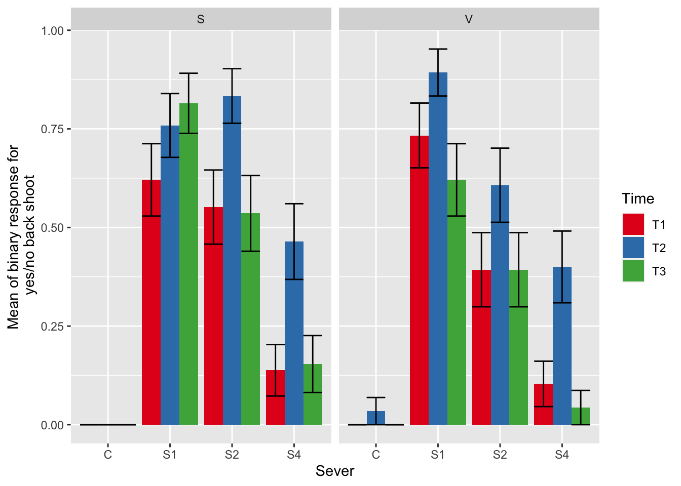
4.1.2 Model selection with leaf area
b_mod91sur<-glmmTMB(backShootBranchBinary~ Sex_90*Sever + Sex_90*Time + Lf_90 + (1|COLONY), data = mayappleData,
                family="binomial")
#this is the global model because it was the largest model that would run
#MuMIn::getAllTerms(b_mod91sur) #this lets us see how to specify terms in the model

dr<-dredge(b_mod91sur, fixed=~cond(Lf_90))

tab <- head(dr, n=10) %>% gt() %>% cols_hide(columns=vars(`disp((Int))`)) %>%
  cols_label(`cond((Int))`="(Intercept)", `cond(Lf_90)`="Lf_90", `cond(Sever)`="Sever", `cond(Sex_90)`="Sex_90", `cond(Time)`="Time", `cond(Sever:Sex_90)`="Sever:Sex_90",  `cond(Sex_90:Time)`= "Sex_90:Time") %>%
  fmt_number(columns = vars(`cond((Int))`, logLik, AICc, delta, weight), decimals = 2) %>%
  fmt_number(columns = vars(`cond(Lf_90)`), decimals = 4) %>%
  tab_spanner(label = "Fit information", columns = vars(df, logLik, AICc, delta, weight)) %>%
  tab_spanner(label = "Non-fixed parameters", columns = vars(`cond((Int))`,  `cond(Lf_90)`, `cond(Sever)`, `cond(Sex_90)`, `cond(Time)`, `cond(Sever:Sex_90)`,  `cond(Sex_90:Time)`)) %>%
  tab_spanner(label = "Fixed parameters", columns = vars(`cond((Int))`,  `cond(Lf_90)`)) %>%
    tab_style(style = cell_fill(color = "lightgrey"), locations = cells_body(columns = everything(),rows = delta <= 2)) %>%
  tab_style(style = cell_fill(color = "darkgrey"), locations = cells_body( columns = everything(), rows = 1))


tab %>% gtsave("back_91_sur_a.png", vwidth=1200) 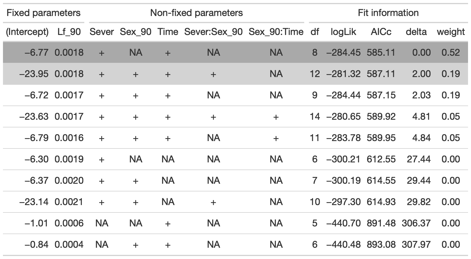
From this round of model selection, when Lf_90 is required to be in the models that are considered, the best model contains Lf_90, Sever, and Time.
4.1.3 Model selection without leaf area
## Fixed terms are "cond((Int))" and "disp((Int))"tab <- head(dr, n=10) %>% gt() %>% cols_hide(columns=vars(`disp((Int))`)) %>%
cols_label(`cond((Int))`="(Intercept)", `cond(Lf_90)`="Lf_90", `cond(Sever)`="Sever", `cond(Sex_90)`="Sex_90", `cond(Time)`="Time", `cond(Sever:Sex_90)`="Sever:Sex_90", `cond(Sex_90:Time)`= "Sex_90:Time") %>%
fmt_number(columns = vars(`cond((Int))`, logLik, AICc, delta, weight), decimals = 2) %>%
fmt_number(columns = vars(`cond(Lf_90)`), decimals = 4) %>%
tab_spanner(label = "Fit information", columns = vars(df, logLik, AICc, delta, weight)) %>%
tab_spanner(label = "Non-fixed parameters", columns = vars(`cond((Int))`, `cond(Lf_90)`, `cond(Sever)`, `cond(Sex_90)`, `cond(Time)`, `cond(Sever:Sex_90)`, `cond(Sex_90:Time)`)) %>%
tab_spanner(label = "Fixed parameters", columns = vars(`cond((Int))`)) %>%
tab_style(style = cell_fill(color = "lightgrey"), locations = cells_body(columns = everything(),rows = delta <= 2)) %>%
tab_style(style = cell_fill(color = "darkgrey"), locations = cells_body( columns = everything(), rows = 1))
tab %>% gtsave("back_91_sur_b.png", vwidth=1200) 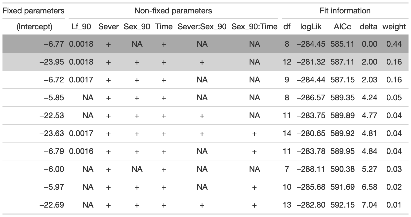
From this round of model selection, when lf_90 is not required to be in the models that are considered, the same best model is returned, with fixed effects of Lf_90, Sever, and Time.
4.1.4 Conclusion
sur_91b_bm<-glmmTMB(backShootBranchBinary~ Sever+Time + Lf_90 +(1|COLONY), data = mayappleData,
                family="binomial")
The best model for the production of a back shoot in 1991 contains fixed effects of Sever, Time, and Lf_90.
4.1.5 Estimated marginal means
The main effect of severing
g1 <- ggplot(data=mayappleData, aes(x=Sever, y=backShootBranchBinary)) +
  geom_bar(stat="summary", fun.y = "mean", position = "dodge") +
  ylab("Mean of binary response for\n producing a shoot/no shoot")

emmeans(sur_91b_bm, pairwise~Sever, type="response" )
## $emmeans
## Sever prob SE df lower.CL upper.CL
## C 0.00382 0.00388 671 0.000518 0.0276
## S1 0.78068 0.03886 671 0.695090 0.8475
## S2 0.57489 0.05008 671 0.474881 0.6691
## S4 0.18015 0.03532 671 0.120800 0.2600
##
## Results are averaged over the levels of: Time
## Confidence level used: 0.95
## Intervals are back-transformed from the logit scale
##
## $contrasts
## contrast odds.ratio SE df t.ratio p.value
## C / S1 0.00108 0.00112 671 -6.581 <.0001
## C / S2 0.00284 0.00292 671 -5.697 <.0001
## C / S4 0.01746 0.01794 671 -3.940 0.0005
## S1 / S2 2.63215 0.66997 671 3.802 0.0009
## S1 / S4 16.19948 4.85008 671 9.302 <.0001
## S2 / S4 6.15447 1.68975 671 6.619 <.0001
##
## Results are averaged over the levels of: Time
## P value adjustment: tukey method for comparing a family of 4 estimates
## Tests are performed on the log odds ratio scale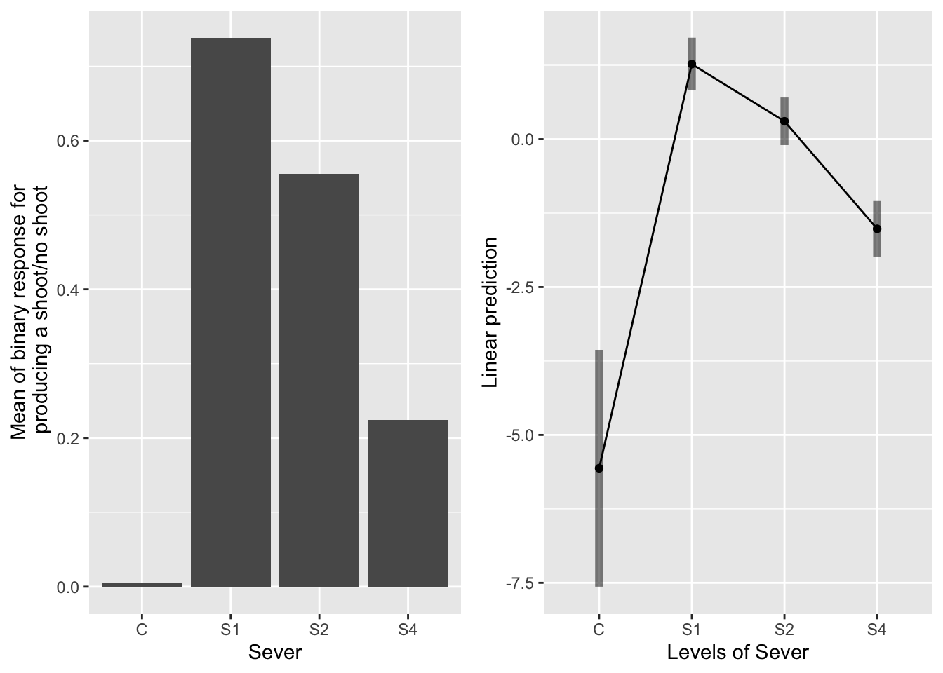 The treatments were significantly different in their production of back shoots. From greatest to least: S1, S2, S4, C.
The main effect of time
g1 <- ggplot(data=mayappleData, aes(x=Time, y=backShootBranchBinary)) +
  geom_bar(stat="summary", fun.y = "mean", position = "dodge") +
  ylab("Mean of binary response for\n producing a shoot/no shoot")

emmeans(sur_91b_bm, pairwise~Time, type="response" )
## $emmeans
## Time prob SE df lower.CL upper.CL
## T1 0.154 0.0432 671 0.0869 0.259
## T2 0.370 0.0747 671 0.2385 0.524
## T3 0.130 0.0380 671 0.0721 0.225
##
## Results are averaged over the levels of: Sever
## Confidence level used: 0.95
## Intervals are back-transformed from the logit scale
##
## $contrasts
## contrast odds.ratio SE df t.ratio p.value
## T1 / T2 0.31 0.0846 671 -4.293 0.0001
## T1 / T3 1.22 0.3272 671 0.724 0.7492
## T2 / T3 3.92 1.0752 671 4.973 <.0001
##
## Results are averaged over the levels of: Sever
## P value adjustment: tukey method for comparing a family of 3 estimates
## Tests are performed on the log odds ratio scale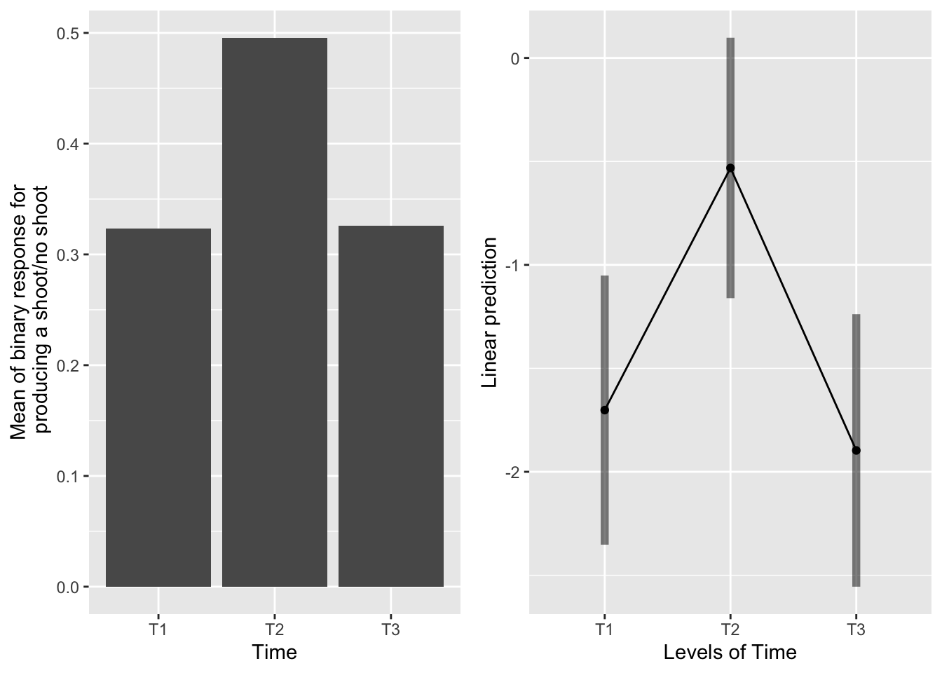 Systems severed at T1 and T3 were equally likely to produce a back shoot. Systems severed at T2 were most likely to produce a back shoot.
The main effect of leaf area
newdat <- expand.grid(Lf_90=seq(min(mayappleData$Lf_90,na.rm=TRUE), max(mayappleData$Lf_90,na.rm=TRUE),len=100),
                     Time = c("T1","T2","T3"),
                     Sever = c("C","S1","S2","S4"),
                     COLONY = mayappleData$COLONY)
newdat$backBinary = predict(sur_91b_bm, newdata=newdat, type="response",re.form=~0)

ggplot(data=mayappleData, aes(x=Lf_90, y=backShootBranchBinary, color=Sever)) +
  geom_point() + geom_line(data=newdat, aes(x=Lf_90, y=backBinary, color=Sever))+
  facet_wrap(~Time) +
  ylab("Mean of binary response for\n producing a shoot/no shoot")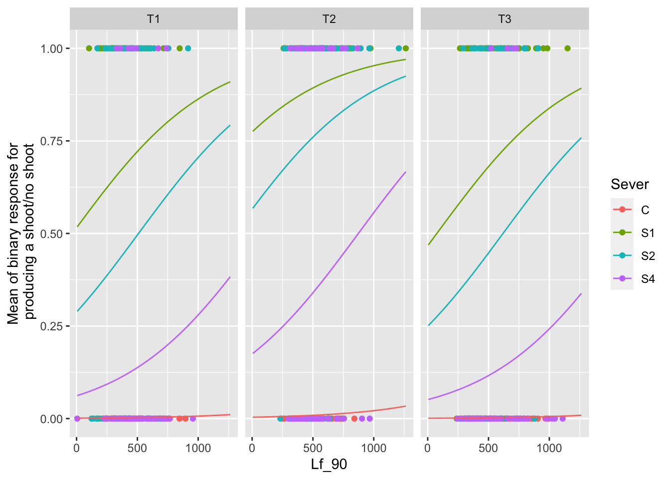
4.2 Leaf area
4.2.1 Conditional leaf area data & visualization
## Warning: NAs introduced by coercionmayappleData <- mayappleData %>%
filter(!is.na(LfBtot_91)) %>%
filter(LfBtot_91>0)
ggplot(data=mayappleData, aes(x=Sever, y=LfBtot_91, fill = Time)) +
stat_summary(fun = mean, geom = "bar",position="dodge") +
stat_summary(fun.data = mean_se, geom = "errorbar", position="dodge")+
facet_wrap(~Sex_90) +
ylab("Mean of total leaf area \n for branches in back shoot of plant") +
scale_fill_brewer(palette="Set1")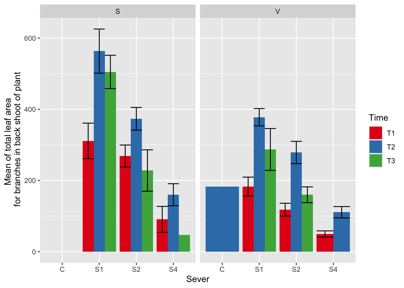
4.2.2 Conditional model selection
b_mod91la.0l<-lmer(LfBtot_91~Sex_90*Time+Sever +Lf_90+(1|COLONY), data = mayappleData, na.action ="na.fail", REML=FALSE)

#this is the global model
#MuMIn::getAllTerms(b_mod91la.0l) #this lets us see how to specify terms in the model

dr<-dredge(b_mod91la.0l)

tab <- head(dr, n=10) %>% gt() %>%
  fmt_number(columns = vars(`(Intercept)`, Lf_90, logLik, AICc, delta, weight), decimals = 2) %>%
  tab_spanner(label = "Fit information", columns = vars(df, logLik, AICc, delta, weight)) %>%
  tab_spanner(label = "Non-fixed parameters", columns = vars(`(Intercept)`,   Lf_90,  Sever, Sex_90, Time,    `Sex_90:Time` )) %>%
  tab_spanner(label = "Fixed parameters", columns = vars(`(Intercept)`,Lf_90)) %>%
    tab_style(style = cell_fill(color = "lightgrey"), locations = cells_body(columns = everything(),rows = delta <= 2)) %>%
  tab_style(style = cell_fill(color = "darkgrey"), locations = cells_body( columns = everything(), rows = 1))


tab %>% gtsave("back_91_leaf_conditional.png", vwidth=1200) 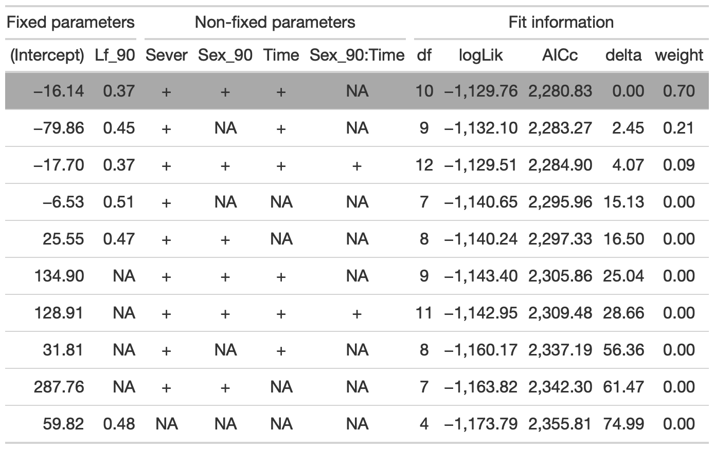
The best model includes Lf_90, Sever, Sex_90, and Time.
4.2.3 Conclusion
4.2.4 Estimated marginal means
the main effect of sex
g1 <- ggplot(data=mayappleData, aes(x=Sex_90, y=LfBtot_91)) +
  geom_bar(stat="summary", fun.y = "mean", position = "dodge") +
  ylab("Mean of total leaf area \n for branches in back of plant")
## Warning: Ignoring unknown parameters: fun.y## Cannot use mode = "kenward-roger" because *pbkrtest* package is not installed## $emmeans
## Sex_90 emmean SE df lower.CL upper.CL
## S 249 37.5 177 175 323
## V 196 38.2 175 120 271
##
## Results are averaged over the levels of: Sever, Time
## Degrees-of-freedom method: satterthwaite
## Confidence level used: 0.95
##
## $contrasts
## contrast estimate SE df t.ratio p.value
## S - V 53.4 24.5 174 2.181 0.0305
##
## Results are averaged over the levels of: Sever, Time
## Degrees-of-freedom method: satterthwaite## Cannot use mode = "kenward-roger" because *pbkrtest* package is not installed## No summary function supplied, defaulting to `mean_se()`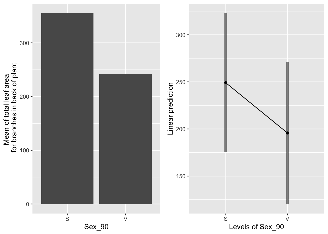
the main effect of time
g1 <- ggplot(data=mayappleData, aes(x=Time, y=LfBtot_91)) +
  geom_bar(stat="summary", fun.y = "mean", position = "dodge") +
  ylab("Mean of total leaf area \n for branches in back of plant")
## Warning: Ignoring unknown parameters: fun.y## Cannot use mode = "kenward-roger" because *pbkrtest* package is not installed## $emmeans
## Time emmean SE df lower.CL upper.CL
## T1 175 40.3 177 95.4 254
## T2 287 35.7 174 216.5 358
## T3 205 41.2 179 124.1 287
##
## Results are averaged over the levels of: Sex_90, Sever
## Degrees-of-freedom method: satterthwaite
## Confidence level used: 0.95
##
## $contrasts
## contrast estimate SE df t.ratio p.value
## T1 - T2 -112.2 25.5 174 -4.404 0.0001
## T1 - T3 -30.6 30.0 174 -1.020 0.5654
## T2 - T3 81.5 26.5 165 3.081 0.0068
##
## Results are averaged over the levels of: Sex_90, Sever
## Degrees-of-freedom method: satterthwaite
## P value adjustment: tukey method for comparing a family of 3 estimates## Cannot use mode = "kenward-roger" because *pbkrtest* package is not installed## No summary function supplied, defaulting to `mean_se()` Systems severed at T2 produce more leaf area than systems severed at T1 or T3, which are equivalent.
the main effect of sever
g1 <- ggplot(data=mayappleData, aes(x=Sever, y=LfBtot_91)) +
  geom_bar(stat="summary", fun.y = "mean", position = "dodge") +
  ylab("Mean of total leaf area \n for branches in back of plant")
## Warning: Ignoring unknown parameters: fun.y## Cannot use mode = "kenward-roger" because *pbkrtest* package is not installed## $emmeans
## Sever emmean SE df lower.CL upper.CL
## C 195 133.7 177.1 -69.3 459
## S1 379 15.8 74.2 347.6 411
## S2 248 18.7 109.0 210.9 285
## S4 68 29.1 165.9 10.6 125
##
## Results are averaged over the levels of: Sex_90, Time
## Degrees-of-freedom method: satterthwaite
## Confidence level used: 0.95
##
## $contrasts
## contrast estimate SE df t.ratio p.value
## C - S1 -184.5 134.2 176 -1.375 0.5166
## C - S2 -53.4 134.5 177 -0.397 0.9787
## C - S4 126.7 135.3 175 0.936 0.7854
## S1 - S2 131.1 21.8 168 6.017 <.0001
## S1 - S4 311.2 30.9 172 10.084 <.0001
## S2 - S4 180.0 31.2 169 5.775 <.0001
##
## Results are averaged over the levels of: Sex_90, Time
## Degrees-of-freedom method: satterthwaite
## P value adjustment: tukey method for comparing a family of 4 estimates## Cannot use mode = "kenward-roger" because *pbkrtest* package is not installed## No summary function supplied, defaulting to `mean_se()`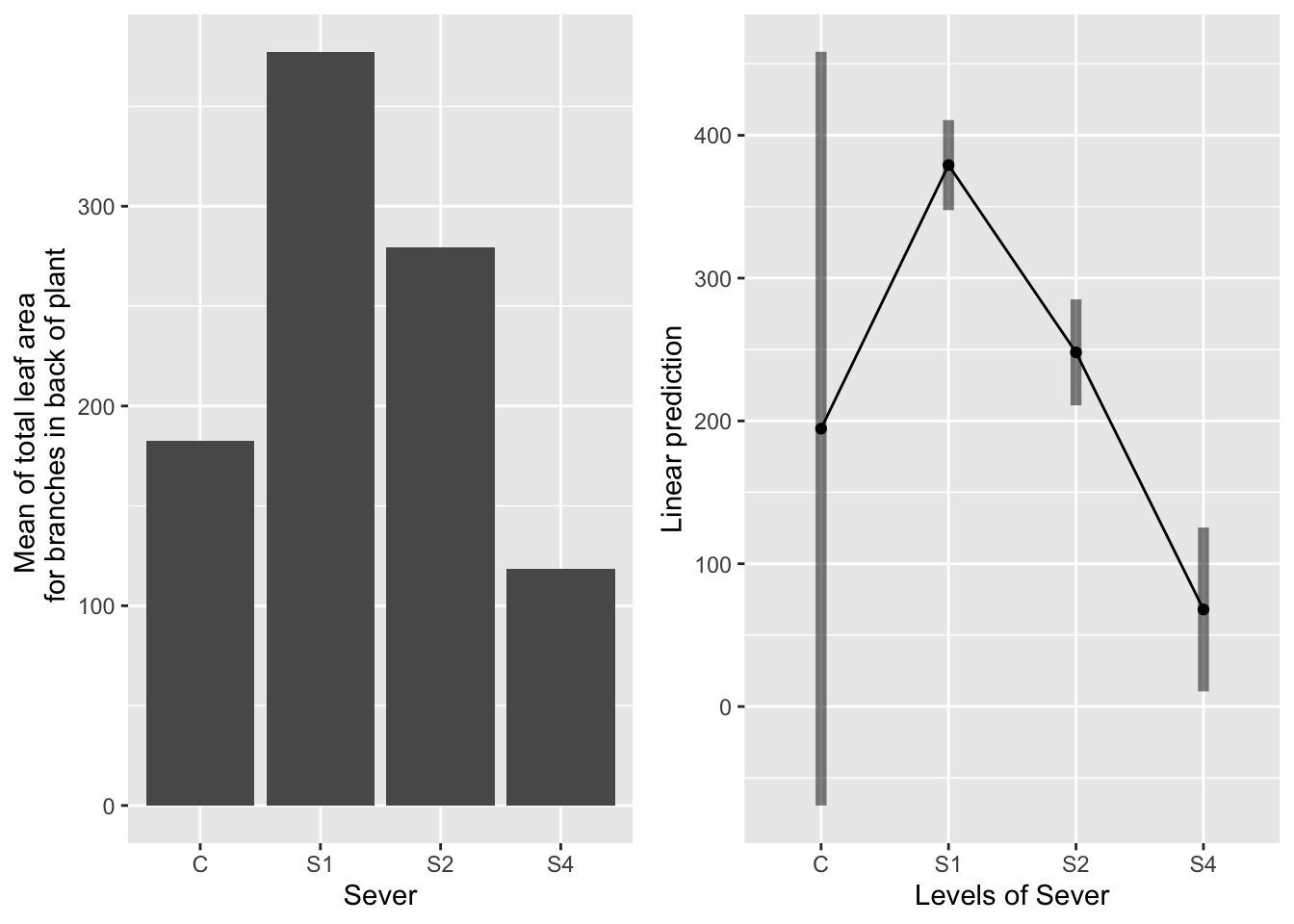 Systems in the control and S4 treatment groups had equally little leaf area in the back. Systems in the S1 treatment had the most leaf area, followed by the S2 systems.
These analyses include the systems with zero leaf area ### Data & visualization
mayappleData$LfBtot_91<-as.numeric(mayappleData$LfBtot_91)

mayappleData <- mayappleData %>%
  filter(!is.na(LfBtot_91))

ggplot(data=mayappleData, aes(x=Sever, y=LfBtot_91, fill = Time)) +
  stat_summary(fun = mean, geom = "bar",position="dodge") +
  stat_summary(fun.data = mean_se, geom = "errorbar", position="dodge")+
  facet_wrap(~Sex_90) +
  ylab("Mean of total leaf area \n for branches in back shoot of plant") +
  scale_fill_brewer(palette="Set1")
4.2.5 Model selection with leaf area
b_mod91la.0l<-lmer(LfBtot_91~Sex_90*Sever*Time +Lf_90+(1|COLONY), data = mayappleData, na.action ="na.fail", REML=FALSE)

#this is the global model
#MuMIn::getAllTerms(b_mod91la.0l) #this lets us see how to specify terms in the model

dr<-dredge(b_mod91la.0l, fixed=~Lf_90)

tab <- head(dr, n=10) %>% gt() %>%
  fmt_number(columns = vars(`(Intercept)`, Lf_90, logLik, AICc, delta, weight), decimals = 2) %>%
  tab_spanner(label = "Fit information", columns = vars(df, logLik, AICc, delta, weight)) %>%
  tab_spanner(label = "Non-fixed parameters", columns = vars(`(Intercept)`,   Lf_90,  Sever, Sex_90, Time,  `Sever:Sex_90`, `Sever:Time`, `Sex_90:Time`, `Sever:Sex_90:Time`)) %>%
  tab_spanner(label = "Fixed parameters", columns = vars(`(Intercept)`,Lf_90)) %>%
    tab_style(style = cell_fill(color = "lightgrey"), locations = cells_body(columns = everything(),rows = delta <= 2)) %>%
  tab_style(style = cell_fill(color = "darkgrey"), locations = cells_body( columns = everything(), rows = 1))


tab %>% gtsave("back_91_leaf_a.png", vwidth=1200) 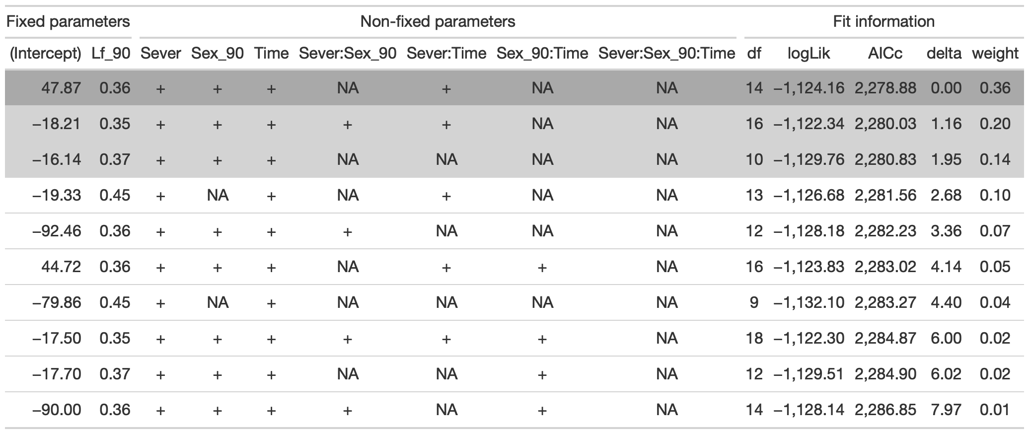
From this round of model selection, when Lf_90 is required to be in the models that are considered, the best model contains fixed effects of Lf_90, Sever, Sex_90, Time, Sever x Sex_90, and Sever x Time (AICc 7512.9).
4.2.6 Model selection without leaf area
## Fixed term is "(Intercept)"## boundary (singular) fit: see ?isSingular
## boundary (singular) fit: see ?isSingular
## boundary (singular) fit: see ?isSingular
## boundary (singular) fit: see ?isSingular## fixed-effect model matrix is rank deficient so dropping 1 column / coefficient
## fixed-effect model matrix is rank deficient so dropping 1 column / coefficient
## fixed-effect model matrix is rank deficient so dropping 1 column / coefficient
## fixed-effect model matrix is rank deficient so dropping 1 column / coefficient## fixed-effect model matrix is rank deficient so dropping 2 columns / coefficients
## fixed-effect model matrix is rank deficient so dropping 2 columns / coefficients
## fixed-effect model matrix is rank deficient so dropping 2 columns / coefficients
## fixed-effect model matrix is rank deficient so dropping 2 columns / coefficients## fixed-effect model matrix is rank deficient so dropping 3 columns / coefficients
## fixed-effect model matrix is rank deficient so dropping 3 columns / coefficients## boundary (singular) fit: see ?isSingular## fixed-effect model matrix is rank deficient so dropping 1 column / coefficient
## fixed-effect model matrix is rank deficient so dropping 1 column / coefficient## fixed-effect model matrix is rank deficient so dropping 2 columns / coefficients
## fixed-effect model matrix is rank deficient so dropping 2 columns / coefficients## fixed-effect model matrix is rank deficient so dropping 3 columns / coefficients
## fixed-effect model matrix is rank deficient so dropping 3 columns / coefficients## fixed-effect model matrix is rank deficient so dropping 6 columns / coefficients
## fixed-effect model matrix is rank deficient so dropping 6 columns / coefficientstab <- head(dr, n=10) %>% gt() %>%
fmt_number(columns = vars(`(Intercept)`, Lf_90, logLik, AICc, delta, weight), decimals = 2) %>%
tab_spanner(label = "Fit information", columns = vars(df, logLik, AICc, delta, weight)) %>%
tab_spanner(label = "Non-fixed parameters", columns = vars(`(Intercept)`, Lf_90, Sever, Sex_90, Time, `Sever:Sex_90`, `Sever:Time`, `Sex_90:Time`, `Sever:Sex_90:Time`)) %>%
tab_spanner(label = "Fixed parameters", columns = vars(`(Intercept)`)) %>%
tab_style(style = cell_fill(color = "lightgrey"), locations = cells_body(columns = everything(),rows = delta <= 2)) %>%
tab_style(style = cell_fill(color = "darkgrey"), locations = cells_body( columns = everything(), rows = 1))
tab %>% gtsave("back_91_leaf_b.png", vwidth=1200) 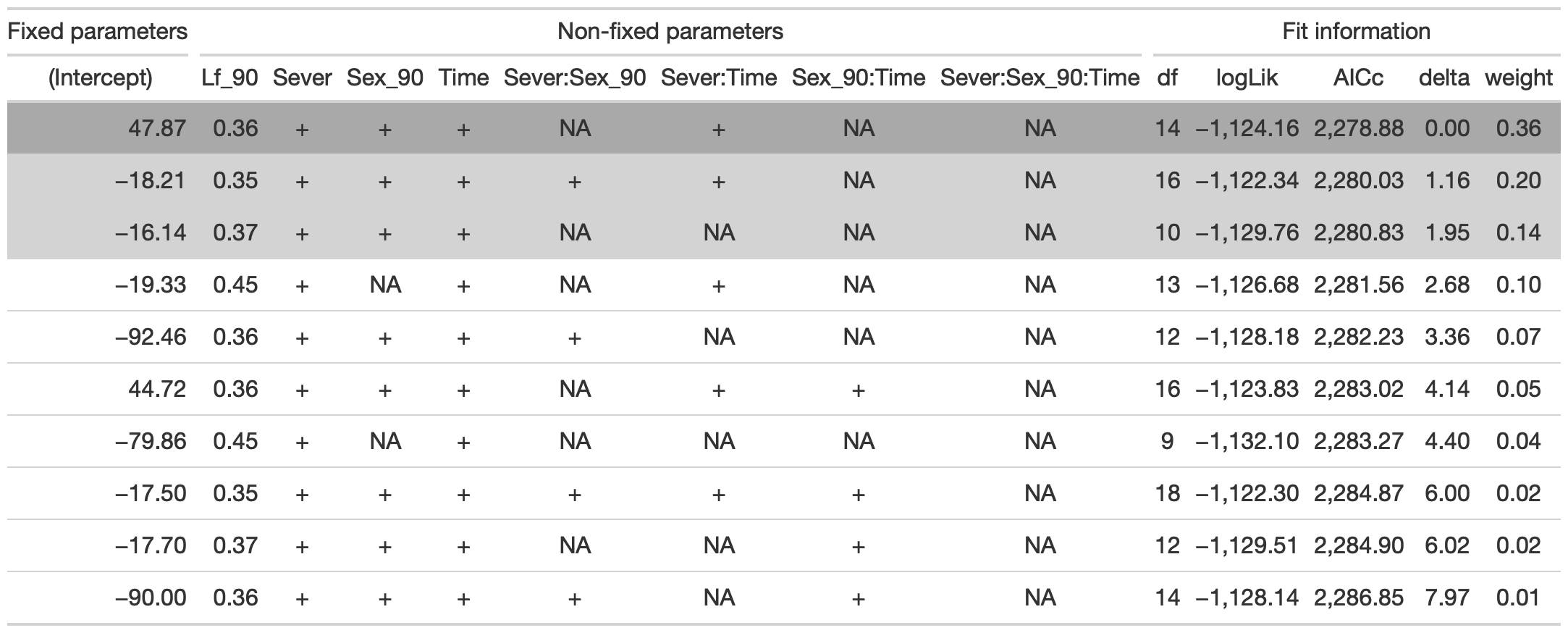
From this round of model selection, when lf_90 is not required to be in the models that are considered, the same best model is returned.
4.2.7 Conclusion
## fixed-effect model matrix is rank deficient so dropping 3 columns / coefficientsThe best model for 1991 back leaf area contains fixed effects of Lf_90, Sever, Sex_90, Time, Sever x Sex_90, and Sever x Time
4.2.8 Estimated marginal means
the sex x sever interaction
g1 <- ggplot(data=mayappleData, aes(x=Sever, y=LfBtot_91, fill=Sex_90)) +
  geom_bar(stat="summary", fun.y = "mean", position = "dodge") +
  ylab("Mean of total leaf area \n for branches in back of plant")
## Warning: Ignoring unknown parameters: fun.y## Cannot use mode = "kenward-roger" because *pbkrtest* package is not installed## $emmeans
## Sever = C:
## Sex_90 emmean SE df lower.CL upper.CL
## S nonEst NA NA NA NA
## V nonEst NA NA NA NA
##
## Sever = S1:
## Sex_90 emmean SE df lower.CL upper.CL
## S 423.7 21.4 132 381.3 466
## V 338.2 23.0 139 292.7 384
##
## Sever = S2:
## Sex_90 emmean SE df lower.CL upper.CL
## S 263.9 23.0 142 218.5 309
## V 217.4 28.8 169 160.5 274
##
## Sever = S4:
## Sex_90 emmean SE df lower.CL upper.CL
## S 61.1 51.0 178 -39.6 162
## V 85.9 60.0 179 -32.5 204
##
## Results are averaged over the levels of: Time
## Degrees-of-freedom method: satterthwaite
## Confidence level used: 0.95
##
## $contrasts
## Sever = C:
## contrast estimate SE df t.ratio p.value
## S - V nonEst NA NA NA NA
##
## Sever = S1:
## contrast estimate SE df t.ratio p.value
## S - V 85.5 31.4 175 2.724 0.0071
##
## Sever = S2:
## contrast estimate SE df t.ratio p.value
## S - V 46.5 34.1 172 1.362 0.1750
##
## Sever = S4:
## contrast estimate SE df t.ratio p.value
## S - V -24.9 52.6 168 -0.473 0.6371
##
## Results are averaged over the levels of: Time
## Degrees-of-freedom method: satterthwaite## Cannot use mode = "kenward-roger" because *pbkrtest* package is not installed## No summary function supplied, defaulting to `mean_se()`## Warning: Removed 2 rows containing missing values (geom_point).## Warning: Removed 2 row(s) containing missing values (geom_path).## Warning: Removed 2 rows containing missing values (geom_segment).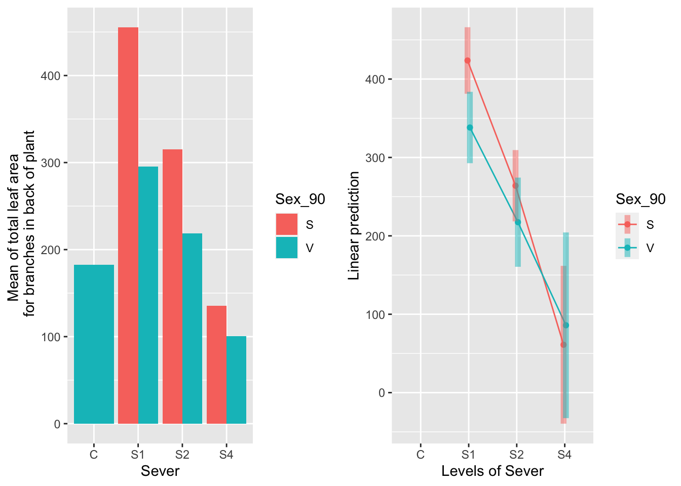
Sexual systems produce a lot more leaf area than vegetative systems for the controls, S1, and S2. This difference is marginally significant at S4.
the sever x time interaction
g1 <- ggplot(data=mayappleData, aes(x=Sever, y=LfBtot_91, fill=Time)) +
  geom_bar(stat="summary", fun.y = "mean", position = "dodge") +
  ylab("Mean of total leaf area \n for branches in back of plant")
## Warning: Ignoring unknown parameters: fun.y## Cannot use mode = "kenward-roger" because *pbkrtest* package is not installed## $emmeans
## Sever = C:
## Time emmean SE df lower.CL upper.CL
## T1 nonEst NA NA NA NA
## T2 nonEst NA NA NA NA
## T3 nonEst NA NA NA NA
##
## Sever = S1:
## Time emmean SE df lower.CL upper.CL
## T1 290.9 26.1 159 239.4 342
## T2 454.4 22.9 155 409.2 500
## T3 397.5 26.5 162 345.2 450
##
## Sever = S2:
## Time emmean SE df lower.CL upper.CL
## T1 245.1 31.5 171 183.0 307
## T2 314.3 22.7 153 269.4 359
## T3 162.6 39.2 179 85.3 240
##
## Sever = S4:
## Time emmean SE df lower.CL upper.CL
## T1 84.2 57.2 177 -28.6 197
## T2 118.3 30.0 172 59.1 178
## T3 18.0 131.0 179 -240.5 277
##
## Results are averaged over the levels of: Sex_90
## Degrees-of-freedom method: satterthwaite
## Confidence level used: 0.95
##
## $contrasts
## Sever = C:
## contrast estimate SE df t.ratio p.value
## T1 - T2 nonEst NA NA NA NA
## T1 - T3 nonEst NA NA NA NA
## T2 - T3 nonEst NA NA NA NA
##
## Sever = S1:
## contrast estimate SE df t.ratio p.value
## T1 - T2 -163.5 33.7 171 -4.850 <.0001
## T1 - T3 -106.6 35.6 171 -2.996 0.0088
## T2 - T3 56.9 32.8 164 1.736 0.1948
##
## Sever = S2:
## contrast estimate SE df t.ratio p.value
## T1 - T2 -69.2 37.1 173 -1.868 0.1511
## T1 - T3 82.5 48.9 174 1.685 0.2137
## T2 - T3 151.7 43.2 168 3.514 0.0016
##
## Sever = S4:
## contrast estimate SE df t.ratio p.value
## T1 - T2 -34.1 63.3 167 -0.539 0.8523
## T1 - T3 66.2 142.1 179 0.466 0.8874
## T2 - T3 100.3 134.5 179 0.746 0.7366
##
## Results are averaged over the levels of: Sex_90
## Degrees-of-freedom method: satterthwaite
## P value adjustment: tukey method for comparing a family of 3 estimates## Cannot use mode = "kenward-roger" because *pbkrtest* package is not installed## No summary function supplied, defaulting to `mean_se()`## Warning: Removed 3 rows containing missing values (geom_point).## Warning: Removed 3 row(s) containing missing values (geom_path).## Warning: Removed 3 rows containing missing values (geom_segment).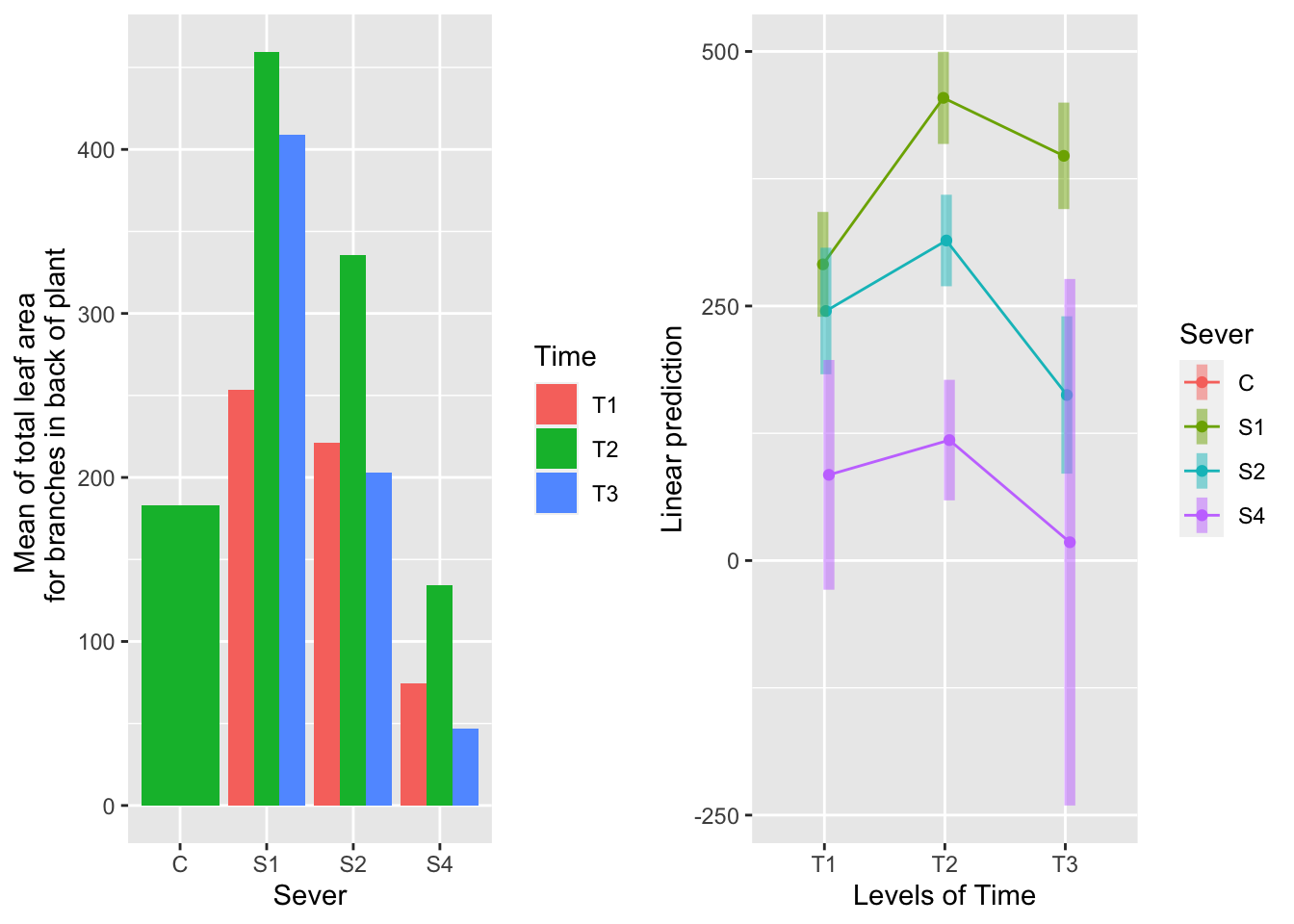
For systems severed at S1, leaf area is greatest for T2, intermediate for T3 and lowest for T1. For systems severed at S2, leaf area is greater at T2 than T1 or T3, which are equivalent.
the main effect of sex
g1 <- ggplot(data=mayappleData, aes(x=Sex_90, y=LfBtot_91)) +
  geom_bar(stat="summary", fun.y = "mean", position = "dodge") +
  ylab("Mean of total leaf area \n for branches in back of plant")
## Warning: Ignoring unknown parameters: fun.y## Cannot use mode = "kenward-roger" because *pbkrtest* package is not installed## NOTE: Results may be misleading due to involvement in interactions## $emmeans
## Sex_90 emmean SE df asymp.LCL asymp.UCL
## S nonEst NA NA NA NA
## V nonEst NA NA NA NA
##
## Results are averaged over the levels of: Sever, Time
## Degrees-of-freedom method: satterthwaite
## Confidence level used: 0.95
##
## $contrasts
## contrast estimate SE df z.ratio p.value
## S - V nonEst NA NA NA NA
##
## Results are averaged over the levels of: Sever, Time
## Degrees-of-freedom method: satterthwaite## Cannot use mode = "kenward-roger" because *pbkrtest* package is not installed
## NOTE: Results may be misleading due to involvement in interactions## No summary function supplied, defaulting to `mean_se()`## Warning: Removed 2 rows containing missing values (geom_point).## Warning: Removed 2 row(s) containing missing values (geom_path).## Warning: Removed 2 rows containing missing values (geom_segment).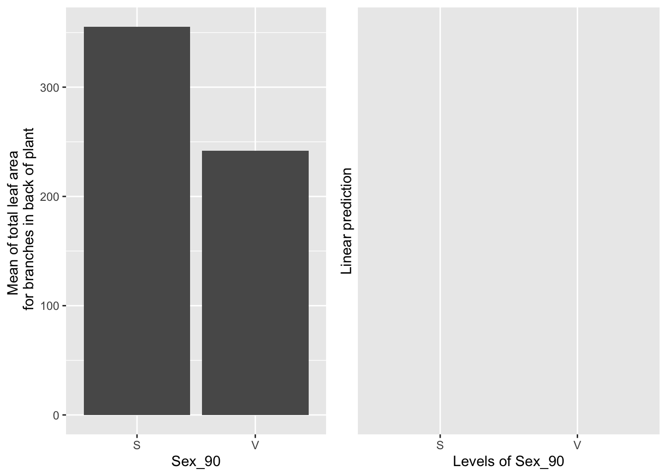
Sexual systems have more leaf area than vegetative systems (raw data), but in the emmeans, which take leaf area in 1990 into account, this difference is not significant.
the main effect of time
g1 <- ggplot(data=mayappleData, aes(x=Time, y=LfBtot_91)) +
  geom_bar(stat="summary", fun.y = "mean", position = "dodge") +
  ylab("Mean of total leaf area \n for branches in back of plant")
## Warning: Ignoring unknown parameters: fun.y## Cannot use mode = "kenward-roger" because *pbkrtest* package is not installed## NOTE: Results may be misleading due to involvement in interactions## $emmeans
## Time emmean SE df lower.CL upper.CL
## T1 nonEst NA NA NA NA
## T2 274 35.1 173 204 343
## T3 nonEst NA NA NA NA
##
## Results are averaged over the levels of: Sex_90, Sever
## Degrees-of-freedom method: satterthwaite
## Confidence level used: 0.95
##
## $contrasts
## contrast estimate SE df z.ratio p.value
## T1 - T2 nonEst NA NA NA NA
## T1 - T3 nonEst NA NA NA NA
## T2 - T3 nonEst NA NA NA NA
##
## Results are averaged over the levels of: Sex_90, Sever
## Degrees-of-freedom method: satterthwaite
## P value adjustment: tukey method for comparing a family of 3 estimates## Cannot use mode = "kenward-roger" because *pbkrtest* package is not installed
## NOTE: Results may be misleading due to involvement in interactions## No summary function supplied, defaulting to `mean_se()`## Warning: Removed 2 rows containing missing values (geom_point).## Warning: Removed 2 row(s) containing missing values (geom_path).## geom_path: Each group consists of only one observation. Do you need to adjust
## the group aesthetic?## Warning: Removed 2 rows containing missing values (geom_segment).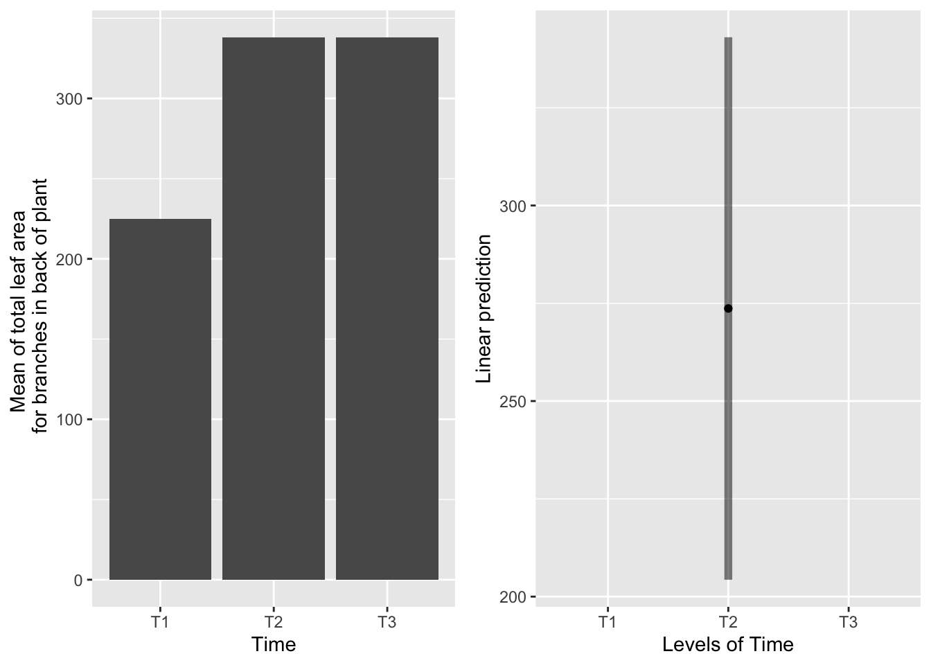 Systems severed at T2 produce more leaf area than systems severed at T1 or T3, which are equivalent.
the main effect of sever
g1 <- ggplot(data=mayappleData, aes(x=Sever, y=LfBtot_91)) +
  geom_bar(stat="summary", fun.y = "mean", position = "dodge") +
  ylab("Mean of total leaf area \n for branches in back of plant")
## Warning: Ignoring unknown parameters: fun.y## Cannot use mode = "kenward-roger" because *pbkrtest* package is not installed## NOTE: Results may be misleading due to involvement in interactions## $emmeans
## Sever emmean SE df lower.CL upper.CL
## C nonEst NA NA NA NA
## S1 380.9 15.8 68.4 349.5 412
## S2 240.7 19.7 114.1 201.7 280
## S4 73.5 49.1 177.8 -23.4 170
##
## Results are averaged over the levels of: Sex_90, Time
## Degrees-of-freedom method: satterthwaite
## Confidence level used: 0.95
##
## $contrasts
## contrast estimate SE df t.ratio p.value
## C - S1 nonEst NA NA NA NA
## C - S2 nonEst NA NA NA NA
## C - S4 nonEst NA NA NA NA
## S1 - S2 140 22.3 168 6.285 <.0001
## S1 - S4 307 50.5 179 6.094 <.0001
## S2 - S4 167 51.6 178 3.239 0.0078
##
## Results are averaged over the levels of: Sex_90, Time
## Degrees-of-freedom method: satterthwaite
## P value adjustment: tukey method for comparing a family of 4 estimates## Cannot use mode = "kenward-roger" because *pbkrtest* package is not installed
## NOTE: Results may be misleading due to involvement in interactions## No summary function supplied, defaulting to `mean_se()`## Warning: Removed 1 rows containing missing values (geom_point).## Warning: Removed 1 row(s) containing missing values (geom_path).## Warning: Removed 1 rows containing missing values (geom_segment).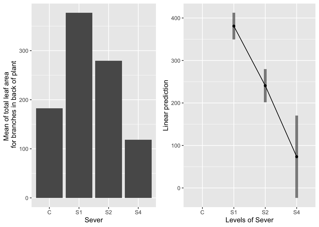 Systems in the control and S4 treatment groups had equally little leaf area in the back. Systems in the S1 treatment had the most leaf area, followed by the S2 systems.
the main effect of leaf area in 1990
ggplot(data=mayappleData, aes(x=Lf_90, y=LfBtot_91, color=Sever)) +
  geom_point() + geom_smooth(method = "lm", se = FALSE)+
  facet_wrap(~Time) +
ylab("Mean of total leaf area \n for branches in back of plant") 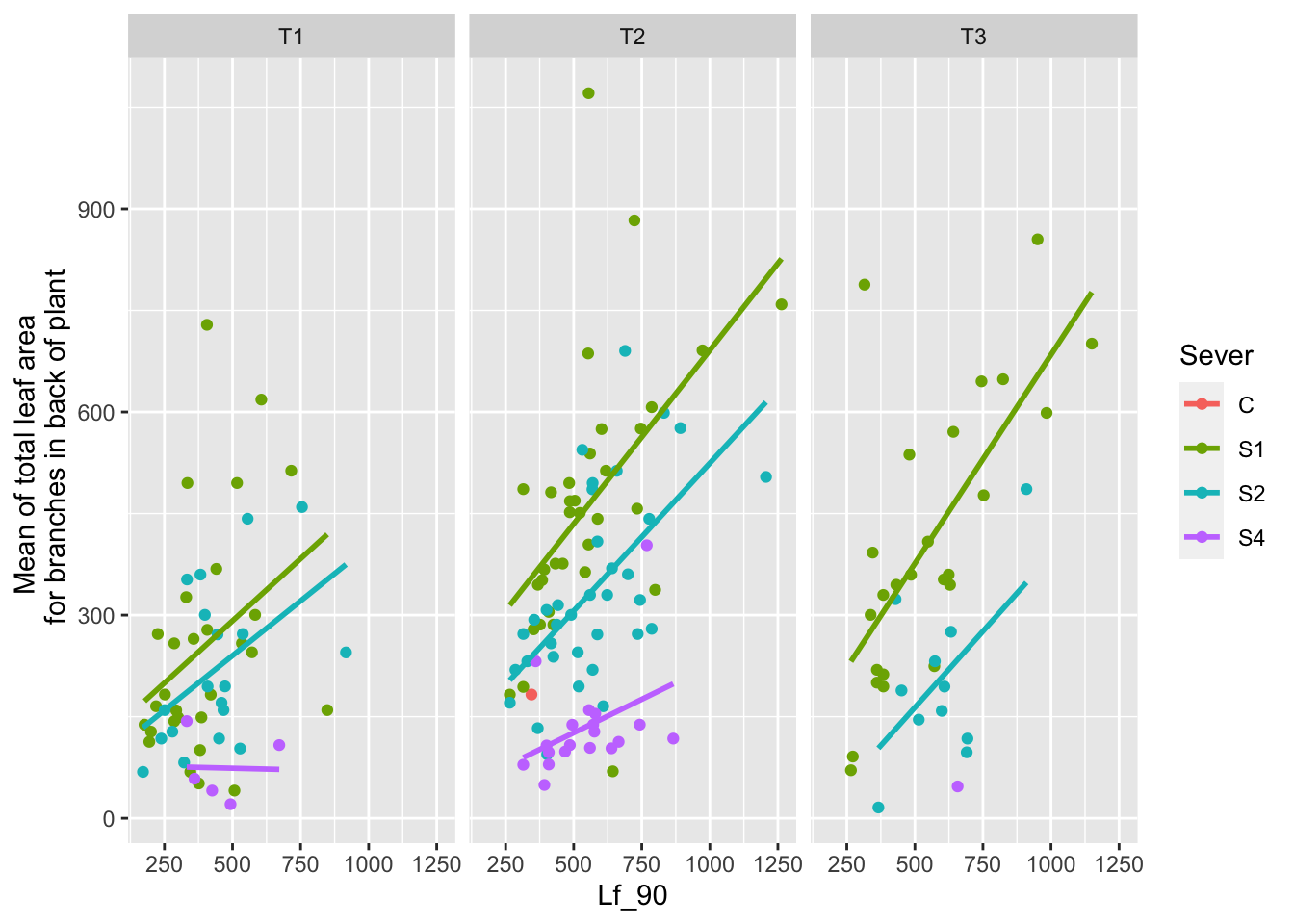
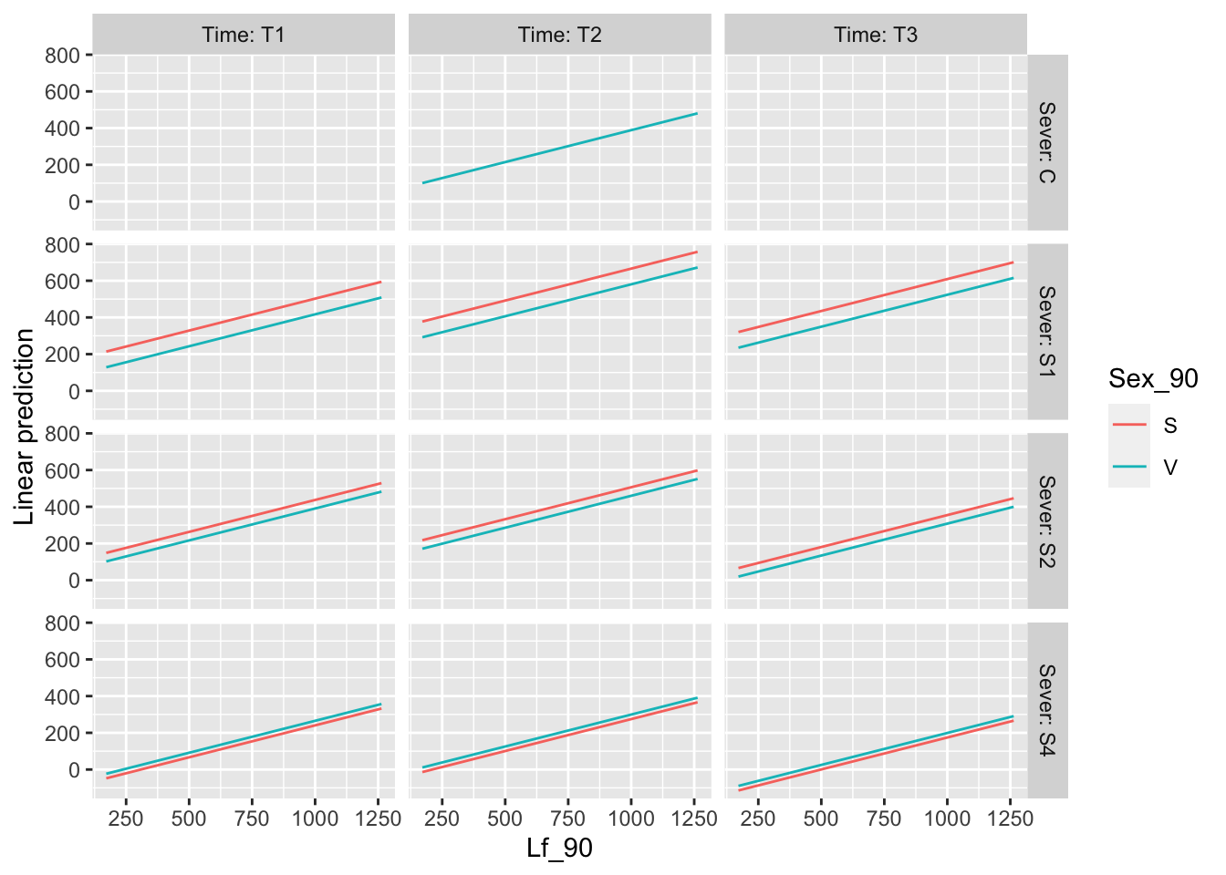 For systems severed at S1 or S2, there is a generally positive relationship between leaf area in the front in 1990 and leaf area in the back in 1991. The differences between sexual and vegetative systems appear larger at S1 and S2 relative to S4 and the control.
plots for MS
g1 <- emmip(b_mod91la.bm,  Sex_90 ~ Sever  ,CIs = TRUE)+ ggtitle("The sex x sever interaction") +
  theme_bw()+theme(plot.title = element_text(face="italic"))+theme(panel.grid.major = element_blank(), panel.grid.minor = element_blank())
## Cannot use mode = "kenward-roger" because *pbkrtest* package is not installedg2 <- emmip(b_mod91la.bm, Time ~ Sever ,CIs = TRUE) +ggtitle("The time x sever interaction")+
theme_bw()+theme(plot.title = element_text(face="italic"))+theme(panel.grid.major = element_blank(), panel.grid.minor = element_blank())## Cannot use mode = "kenward-roger" because *pbkrtest* package is not installedg3 <- emmip(b_mod91la.bm, ~ Sex_90 ,CIs = TRUE) +ggtitle("The main effect of sex")+
theme_bw()+theme(plot.title = element_text(face="italic"))+theme(panel.grid.major = element_blank(), panel.grid.minor = element_blank())## Cannot use mode = "kenward-roger" because *pbkrtest* package is not installed## NOTE: Results may be misleading due to involvement in interactionsg4 <- emmip(b_mod91la.bm, ~ Sever ,CIs = TRUE) + ggtitle("The main effect of sever") +
theme_bw()+theme(plot.title = element_text(face="italic"))+theme(panel.grid.major = element_blank(), panel.grid.minor = element_blank())## Cannot use mode = "kenward-roger" because *pbkrtest* package is not installed
## NOTE: Results may be misleading due to involvement in interactionsg5 <- emmip(b_mod91la.bm, ~ Time ,CIs = TRUE) + ggtitle("The main effect of time") +
theme_bw()+theme(plot.title = element_text(face="italic"))+theme(panel.grid.major = element_blank(), panel.grid.minor = element_blank())## Cannot use mode = "kenward-roger" because *pbkrtest* package is not installed
## NOTE: Results may be misleading due to involvement in interactionsmylist <- list(Lf_90=seq(150,1250,by=100))
g6 <- emmip(b_mod91la.bm, ~ Lf_90 , at=mylist, CIs = TRUE) + ggtitle("The main effect of Lf_1990") +
theme_bw()+theme(plot.title = element_text(face="italic"))+theme(panel.grid.major = element_blank(), panel.grid.minor = element_blank())## Cannot use mode = "kenward-roger" because *pbkrtest* package is not installedlibrary("cowplot")
ggdraw()+
draw_plot(g1, x=0, y=0.5, width = .5, height = .5)+
draw_plot(g2, x=0, y=0, width = 0.5, height = 0.5 ) +
draw_plot(g3, x=0.5, y=0.75, width = 0.5, height = 0.25) +
draw_plot(g4, x=0.5, y=0.5, width = 0.5, height = 0.25) +
draw_plot(g5, x=0.5, y=0.25,width = 0.5, height = 0.25 )+
draw_plot(g6, x=0.5, y=0,width = 0.5, height = 0.25 )## Warning: Removed 2 rows containing missing values (geom_point).## Warning: Removed 2 row(s) containing missing values (geom_path).## Warning: Removed 2 rows containing missing values (geom_segment).## Warning: Removed 3 rows containing missing values (geom_point).## Warning: Removed 3 row(s) containing missing values (geom_path).## Warning: Removed 3 rows containing missing values (geom_segment).## Warning: Removed 2 rows containing missing values (geom_point).## Warning: Removed 2 row(s) containing missing values (geom_path).## Warning: Removed 2 rows containing missing values (geom_segment).## Warning: Removed 1 rows containing missing values (geom_point).## Warning: Removed 1 row(s) containing missing values (geom_path).## Warning: Removed 1 rows containing missing values (geom_segment).## Warning: Removed 2 rows containing missing values (geom_point).## Warning: Removed 2 row(s) containing missing values (geom_path).## geom_path: Each group consists of only one observation. Do you need to adjust
## the group aesthetic?## Warning: Removed 2 rows containing missing values (geom_segment).## Warning: Removed 6 rows containing missing values (geom_point).## Warning: Removed 6 row(s) containing missing values (geom_path).## Warning: Removed 6 rows containing missing values (geom_segment).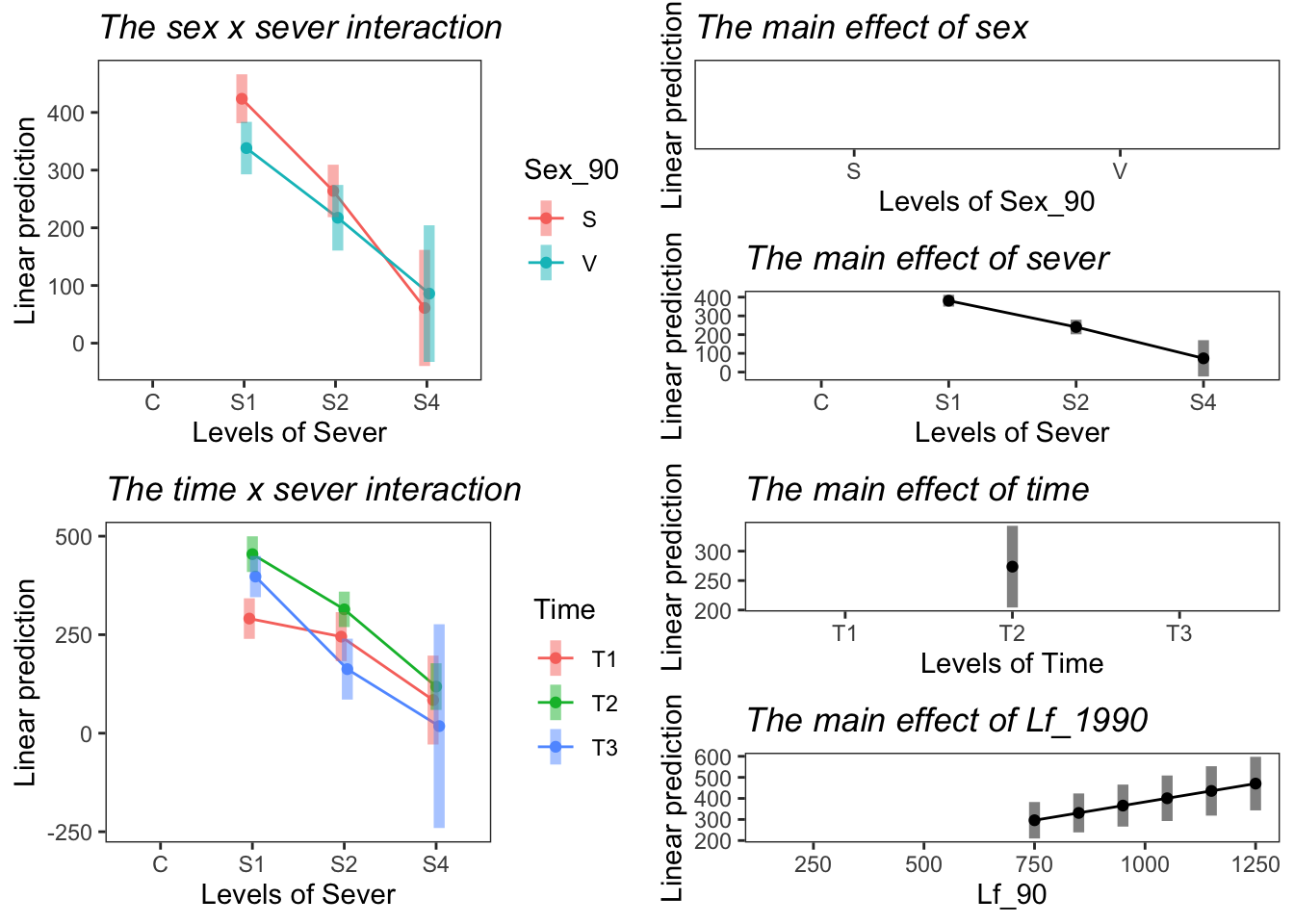
4.3 Branching
4.3.1 Data & visualization
# filter the dataset to only plants that are alive (1 or more branches)
# create binary variable for plants that are have 1 branch (0) or more than 1 branch (1)
# append new variable to the new (filtered) dataframe
mayappleAliveData <- mayappleData %>%
  filter(!is.na(Lf_90)) %>%
  dplyr::filter(brnoB_91>=1) %>%
  dplyr::mutate(branchingBinary=ifelse(brnoB_91>1,1,0))

# create a plot showing the mean of the binary response variable in each category
# interpretation for values = 0, all responses were 0 in that category (all plants have 1 branch)
# interpretation for values = 1, all responses were 1 in that category (all plants have >1 branch)
ggplot(data=mayappleAliveData, aes(x=Sever, y=branchingBinary, fill = Time)) +
   stat_summary(fun = mean, geom = "bar",position="dodge") +
  stat_summary(fun.data = mean_se, geom = "errorbar", position="dodge")+
  facet_wrap(~Sex_90) +
  ylab("Mean of binary response for\n not branching/branching \n on back shoot") +
  scale_fill_brewer(palette="Set1")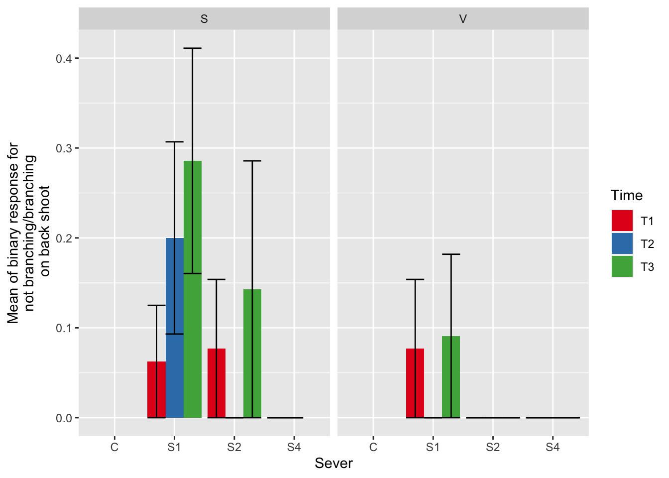
4.3.2 Model selection with leaf area
b_mod91brdl<-glmmTMB(branchingBinary~ Sex_90*Sever + Time + Lf_90 +  (1|COLONY), data = mayappleAliveData,
                family="binomial")

#this is the global model because this is the largest model we could fit with Lf_90 included. I have double-checked and this was the only model with a two-way interaction that ran.
#MuMIn::getAllTerms(b_mod91brdl) #this lets us see how to specify terms in the model

dr<-dredge(b_mod91brdl, fixed=~cond(Lf_90))
knitr::kable(head(dr, n=10)) %>%
  kable_styling() %>%
scroll_box(width = "100%", box_css = "border: 0px;")| cond((Int)) | disp((Int)) | cond(Lf_90) | cond(Sever) | cond(Sex_90) | cond(Time) | cond(Sever:Sex_90) | df | logLik | AICc | delta | weight | |
|---|---|---|---|---|---|---|---|---|---|---|---|---|
| 8 | -7.919347 |
|
0.0018494 |
|
|
|
NA | 8 | -32.62054 | 82.09314 | 0.0000000 | 0.408810786 |
| 4 | -2.837691 |
|
0.0011234 |
|
|
NA | NA | 6 | -35.01578 | 82.52278 | 0.4296347 | 0.329783070 |
| 2 | -4.193048 |
|
0.0029514 |
|
NA | NA | NA | 5 | -37.56321 | 85.47525 | 3.3821071 | 0.075354140 |
| 6 | -4.338055 |
|
0.0033438 |
|
NA |
|
NA | 7 | -35.76591 | 86.19065 | 4.0975010 | 0.052694016 |
| 16 | -7.742156 |
|
0.0019329 |
|
|
|
|
10 | -32.55770 | 86.43277 | 4.3396214 | 0.046685878 |
| 12 | -2.893553 |
|
0.0011944 |
|
|
NA |
|
8 | -34.81249 | 86.47705 | 4.3839039 | 0.045663554 |
| 7 | -3.143551 |
|
0.0005370 | NA |
|
|
NA | 6 | -37.84619 | 88.18361 | 6.0904619 | 0.019453393 |
| 5 | -4.206869 |
|
0.0023650 | NA | NA |
|
NA | 5 | -39.65179 | 89.65241 | 7.5592641 | 0.009333596 |
| 3 | -3.106581 |
|
0.0008878 | NA |
|
NA | NA | 4 | -40.86409 | 89.95940 | 7.8662516 | 0.008005482 |
| 1 | -4.205829 |
|
0.0022635 | NA | NA | NA | NA | 3 | -42.55195 | 91.24183 | 9.1486910 | 0.004216085 |
From this round of model selection, when Lf_90 is required to be in the models that are considered, there are two models within 2 AICc units: (1) Lf_90, Sever, Sex_90, and Time (AICc 82.1); (2) Lf_90, Sever, and Sex_90 (AICc 82.5).
4.3.3 Model selection without leaf area
dr<-dredge(b_mod91brdl)
knitr::kable(head(dr, n=10)) %>%
  kable_styling() %>%
scroll_box(width = "100%", box_css = "border: 0px;")| cond((Int)) | disp((Int)) | cond(Lf_90) | cond(Sever) | cond(Sex_90) | cond(Time) | cond(Sever:Sex_90) | df | logLik | AICc | delta | weight | |
|---|---|---|---|---|---|---|---|---|---|---|---|---|
| 15 | -6.954342 |
|
NA |
|
|
|
NA | 7 | -32.70228 | 80.06339 | 0.0000000 | 0.35424997 |
| 7 | -2.112184 |
|
NA |
|
|
NA | NA | 5 | -35.14097 | 80.63077 | 0.5673806 | 0.26675016 |
| 16 | -7.919347 |
|
0.0018494 |
|
|
|
NA | 8 | -32.62054 | 82.09314 | 2.0297555 | 0.12839675 |
| 8 | -2.837691 |
|
0.0011234 |
|
|
NA | NA | 6 | -35.01578 | 82.52278 | 2.4593902 | 0.10357621 |
| 31 | -2.886490 |
|
NA |
|
|
|
|
9 | -32.74997 | 84.57138 | 4.5079876 | 0.03718885 |
| 23 | -2.120587 |
|
NA |
|
|
NA |
|
7 | -34.95681 | 84.57244 | 4.5090478 | 0.03716914 |
| 4 | -4.193048 |
|
0.0029514 |
|
NA | NA | NA | 5 | -37.56321 | 85.47525 | 5.4118626 | 0.02366676 |
| 13 | -2.865559 |
|
NA | NA |
|
|
NA | 5 | -37.87598 | 86.10080 | 6.0374107 | 0.01731023 |
| 12 | -4.338055 |
|
0.0033438 |
|
NA |
|
NA | 7 | -35.76591 | 86.19065 | 6.1272565 | 0.01654981 |
| 3 | -2.462958 |
|
NA |
|
NA | NA | NA | 4 | -39.06861 | 86.36843 | 6.3050447 | 0.01514212 |
From this round of model selection, when Lf_90 is not required to be in the models that are considered, there are two models within 2 AICc units: (1) Sever, Sex_90, and Time (AICc 80.1); (2) Sever and Sex_90 (AICc 80.6).
4.3.4 Conclusion
b_mod91br_bm<-glmmTMB(branchingBinary~ Sex_90+Sever +  (1|COLONY), data = mayappleAliveData,
                family="binomial")
The simplest model with the lowest AICc includes fixed effects of Sever and Sex_90.
4.3.5 Estimated marginal means
Below are the relevant visualizations of the best model:
the main effect of sex
g1 <- ggplot(data=mayappleAliveData, aes(x=Sex_90, y=branchingBinary)) +
  geom_bar(stat="summary", fun.y = "mean", position = "dodge") +
  ylab("Mean of binary response for\n not branching/branching ")

emmeans(b_mod91br_bm, pairwise~Sex_90, type="response")
## $emmeans
## Sex_90 prob SE df lower.CL upper.CL
## S 2.79e-04 0.08561 173 2.22e-16 1
## V 2.36e-05 0.00722 173 2.22e-16 1
##
## Results are averaged over the levels of: Sever
## Confidence level used: 0.95
## Intervals are back-transformed from the logit scale
##
## $contrasts
## contrast odds.ratio SE df t.ratio p.value
## S / V 11.9 13.8 173 2.123 0.0352
##
## Results are averaged over the levels of: Sever
## Tests are performed on the log odds ratio scale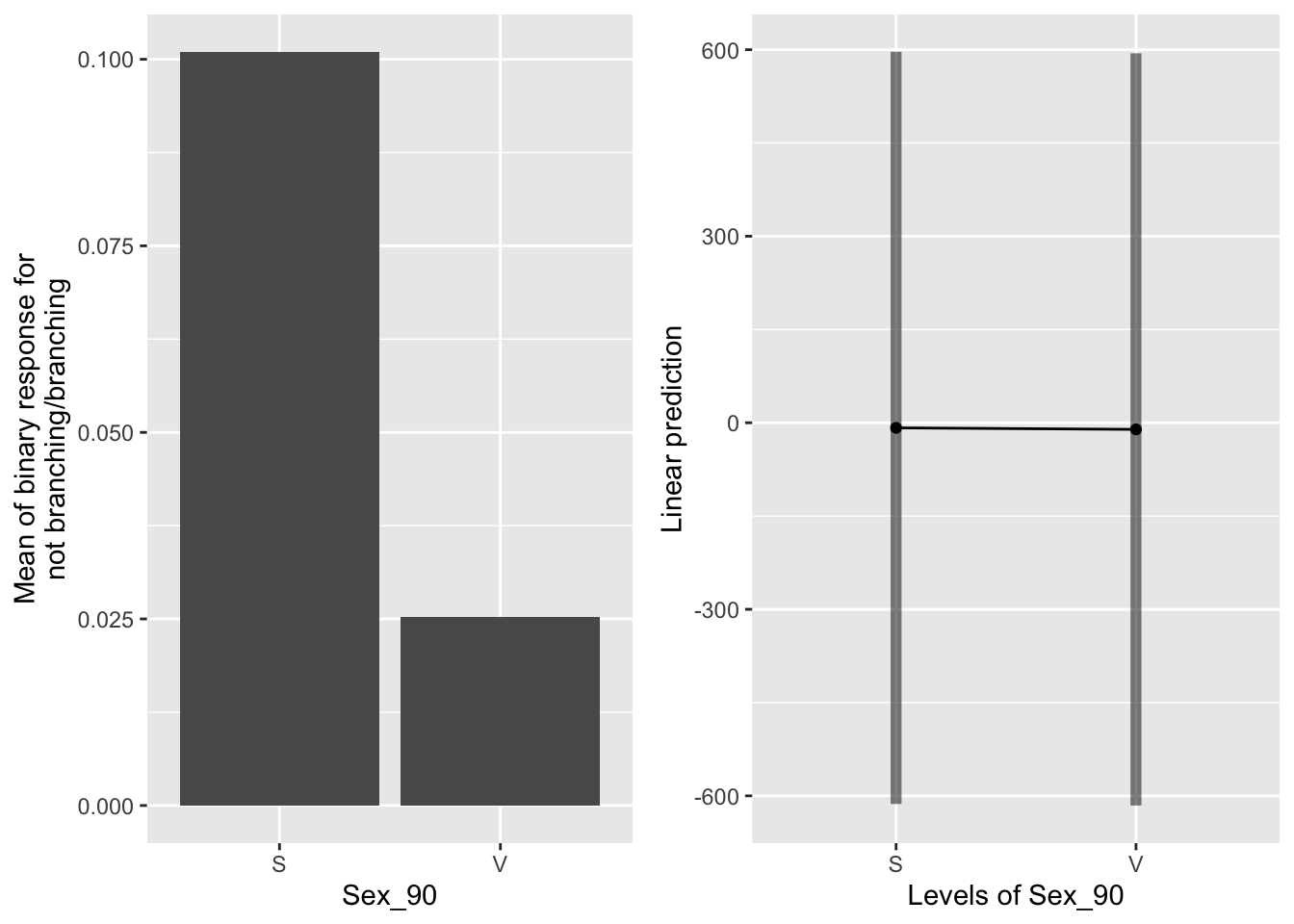 Sexual systems in 1990 were more likely to have branches in the back system in 1991.
the main effect of sever
g1 <- ggplot(data=mayappleAliveData, aes(x=Sever, y=branchingBinary)) +
  geom_bar(stat="summary", fun.y = "mean", position = "dodge") +
  ylab("Mean of binary response for\n not branching/branching ")

emmeans(b_mod91br_bm, pairwise~Sever, type="response")
## $emmeans
## Sever prob SE df lower.CL upper.CL
## S1 0.03393 3.63e-02 173 3.93e-03 0.238
## S2 0.00322 5.78e-03 173 9.25e-05 0.101
## S4 0.00000 4.33e-06 173 0.00e+00 1.000
##
## Results are averaged over the levels of: Sex_90
## Confidence level used: 0.95
## Intervals are back-transformed from the logit scale
##
## $contrasts
## contrast odds.ratio SE df t.ratio p.value
## S1 / S2 11 1.20e+01 173 2.177 0.0780
## S1 / S4 7457316 6.86e+09 173 0.017 0.9998
## S2 / S4 685949 6.31e+08 173 0.015 0.9999
##
## Results are averaged over the levels of: Sex_90
## P value adjustment: tukey method for comparing a family of 3 estimates
## Tests are performed on the log odds ratio scale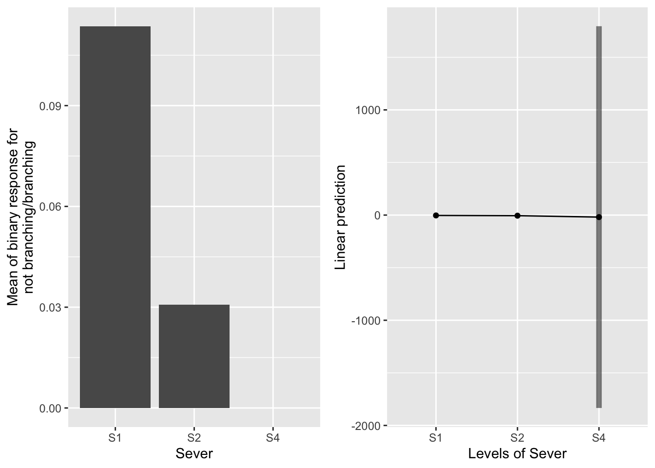 S1 systems are somewhat more likely than S2 systems to branch. I think there were no S4 systems that branched, which makes the comparisons challenging.
4.4 Sexual status
4.4.1 Data & visualization
# filter dataset to plants that have 1 or more branches
# recode the branch sex variables so that for each branch
# a vegetative branch is recorded as a 0
# a sexual branch is recorded as a 0
# sum across the rows to total the number of sexual branches
mayappleSexData <- mayappleDatasetFull %>%
  filter(!is.na(Lf_90)) %>%
  dplyr::filter(brnoB_91==1|brnoB_91==2|brnoB_91==3) %>%
  dplyr::mutate(SexB1_91 = as.numeric(ifelse(SexB1_91=="V",0,1)),
                SexB2_91 = as.numeric(ifelse(SexB2_91=="V",0,1))) %>%
  dplyr::rowwise() %>%
  dplyr::mutate(numberSexualBranches = sum(SexB1_91, SexB2_91, na.rm=TRUE))

mayappleSexData$SexBr<-0
mayappleSexData$SexBr[mayappleSexData$numberSexualBranches==1|mayappleSexData$numberSexualBranches==2]<-1


#removing the control systems:
mayappleSexData <- mayappleSexData %>%
  filter(Sever !="C")

#again this only removes one system

ggplot(data=mayappleSexData, aes(x=Sever, y=numberSexualBranches, fill = Time)) +
   stat_summary(fun = mean, geom = "bar",position="dodge") +
  stat_summary(fun.data = mean_se, geom = "errorbar", position="dodge")+
  facet_wrap(~Sex_90) +
  ylab("Mean of binary variable for number of sexual branches\n per plant on back shoot") +
  scale_fill_brewer(palette="Set1")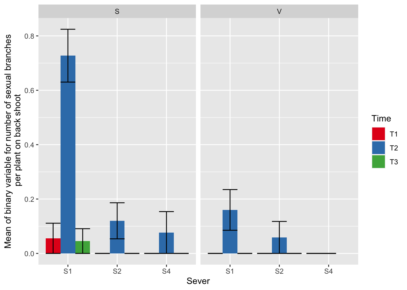
4.4.2 Model selection with leaf area, global model 1
b_mod91sexdl<-glmmTMB(SexBr~ Sex_90*Sever + Time + Lf_90 +  (1|COLONY), data = mayappleSexData,
                family="binomial")
#this is the global model because this was the largest model we could fit with Lf_90
#MuMIn::getAllTerms(b_mod91sexdl) #this lets us see how to specify terms in the model

dr<-dredge(b_mod91sexdl, fixed=~cond(Lf_90))
knitr::kable(head(dr, n=10)) %>%
  kable_styling() %>%
scroll_box(width = "100%", box_css = "border: 0px;")| cond((Int)) | disp((Int)) | cond(Lf_90) | cond(Sever) | cond(Sex_90) | cond(Time) | cond(Sever:Sex_90) | df | logLik | AICc | delta | weight | |
|---|---|---|---|---|---|---|---|---|---|---|---|---|
| 8 | -5.717898 |
|
0.0040367 |
|
|
|
NA | 8 | -46.18920 | 108.9544 | 0.000000 | 7.097358e-01 |
| 16 | -5.758167 |
|
0.0041612 |
|
|
|
|
10 | -45.06359 | 111.0143 | 2.059868 | 2.533973e-01 |
| 6 | -7.219901 |
|
0.0065515 |
|
NA |
|
NA | 7 | -50.21170 | 114.8696 | 5.915203 | 3.686606e-02 |
| 7 | -5.384957 |
|
0.0028126 | NA |
|
|
NA | 6 | -62.29796 | 136.9293 | 27.974845 | 5.976355e-07 |
| 5 | -6.371715 |
|
0.0042211 | NA | NA |
|
NA | 5 | -64.38273 | 139.0026 | 30.048206 | 2.119394e-07 |
| 4 | -3.170869 |
|
0.0034587 |
|
|
NA | NA | 6 | -69.41181 | 151.1570 | 42.202553 | 4.863273e-10 |
| 2 | -4.219714 |
|
0.0046840 |
|
NA | NA | NA | 5 | -70.71533 | 151.6678 | 42.713409 | 3.767019e-10 |
| 12 | -3.174440 |
|
0.0035024 |
|
|
NA |
|
8 | -68.97898 | 154.5340 | 45.579549 | 8.987181e-11 |
| 3 | -3.796268 |
|
0.0031994 | NA |
|
NA | NA | 4 | -77.86262 | 163.8827 | 54.928303 | 8.386239e-13 |
| 1 | -4.583886 |
|
0.0040985 | NA | NA | NA | NA | 3 | -78.92349 | 163.9411 | 54.986685 | 8.144977e-13 |
From this round of model selection, when Lf_90 is required to be in the models that are considered, the best model contains fixed effects of Lf_90, Sever, Sex_90, and Time.
4.4.3 Model selection without leaf area, global model 1
dr<-dredge(b_mod91sexdl)
knitr::kable(head(dr, n=10)) %>%
  kable_styling() %>%
scroll_box(width = "100%", box_css = "border: 0px;")| cond((Int)) | disp((Int)) | cond(Lf_90) | cond(Sever) | cond(Sex_90) | cond(Time) | cond(Sever:Sex_90) | df | logLik | AICc | delta | weight | |
|---|---|---|---|---|---|---|---|---|---|---|---|---|
| 16 | -5.717898 |
|
0.0040367 |
|
|
|
NA | 8 | -46.18920 | 108.9544 | 0.000000 | 5.331288e-01 |
| 32 | -5.758167 |
|
0.0041612 |
|
|
|
|
10 | -45.06359 | 111.0143 | 2.059868 | 1.903432e-01 |
| 15 | -3.641204 |
|
NA |
|
|
|
NA | 7 | -48.32295 | 111.0921 | 2.137713 | 1.830769e-01 |
| 31 | -3.676316 |
|
NA |
|
|
|
|
9 | -47.20888 | 113.1407 | 4.186245 | 6.573558e-02 |
| 12 | -7.219901 |
|
0.0065515 |
|
NA |
|
NA | 7 | -50.21170 | 114.8696 | 5.915203 | 2.769250e-02 |
| 11 | -4.125660 |
|
NA |
|
NA |
|
NA | 6 | -58.39689 | 129.1271 | 20.172709 | 2.220158e-05 |
| 14 | -5.384957 |
|
0.0028126 | NA |
|
|
NA | 6 | -62.29796 | 136.9293 | 27.974845 | 4.489229e-07 |
| 13 | -3.909540 |
|
NA | NA |
|
|
NA | 5 | -64.24656 | 138.7303 | 29.775862 | 1.824257e-07 |
| 10 | -6.371715 |
|
0.0042211 | NA | NA |
|
NA | 5 | -64.38273 | 139.0026 | 30.048206 | 1.592015e-07 |
| 9 | -4.425548 |
|
NA | NA | NA |
|
NA | 4 | -70.31444 | 148.7864 | 39.831946 | 1.195184e-09 |
From this round of model selection, when Lf_90 is not required to be in the models that are considered, the same best model is returned
4.4.4 Conclusion from global model 1
mod91sexbm<-glmmTMB(SexBr~ Sex_90+Sever+Time+ Lf_90 + (1|COLONY), data = mayappleSexData,
                family="binomial")
The best model has main effects of Lf_90, Sex_90, Sever, and Time.
4.4.5 Estimated marginal means
the main effect of sex
g1 <- ggplot(data=mayappleSexData, aes(x=Sex_90, y=SexBr)) +
  geom_bar(stat="summary", fun.y = "mean", position = "dodge") +
  ylab("Mean of binary variable for having zero vs. one or more sexual shoots")

emmeans(mod91sexbm, pairwise~Sex_90, type="response")
## $emmeans
## Sex_90 prob SE df lower.CL upper.CL
## S 0.006167 0.00669 251 7.23e-04 0.0505
## V 0.000708 0.00104 251 3.93e-05 0.0126
##
## Results are averaged over the levels of: Sever, Time
## Confidence level used: 0.95
## Intervals are back-transformed from the logit scale
##
## $contrasts
## contrast odds.ratio SE df t.ratio p.value
## S / V 8.76 7.37 251 2.579 0.0105
##
## Results are averaged over the levels of: Sever, Time
## Tests are performed on the log odds ratio scale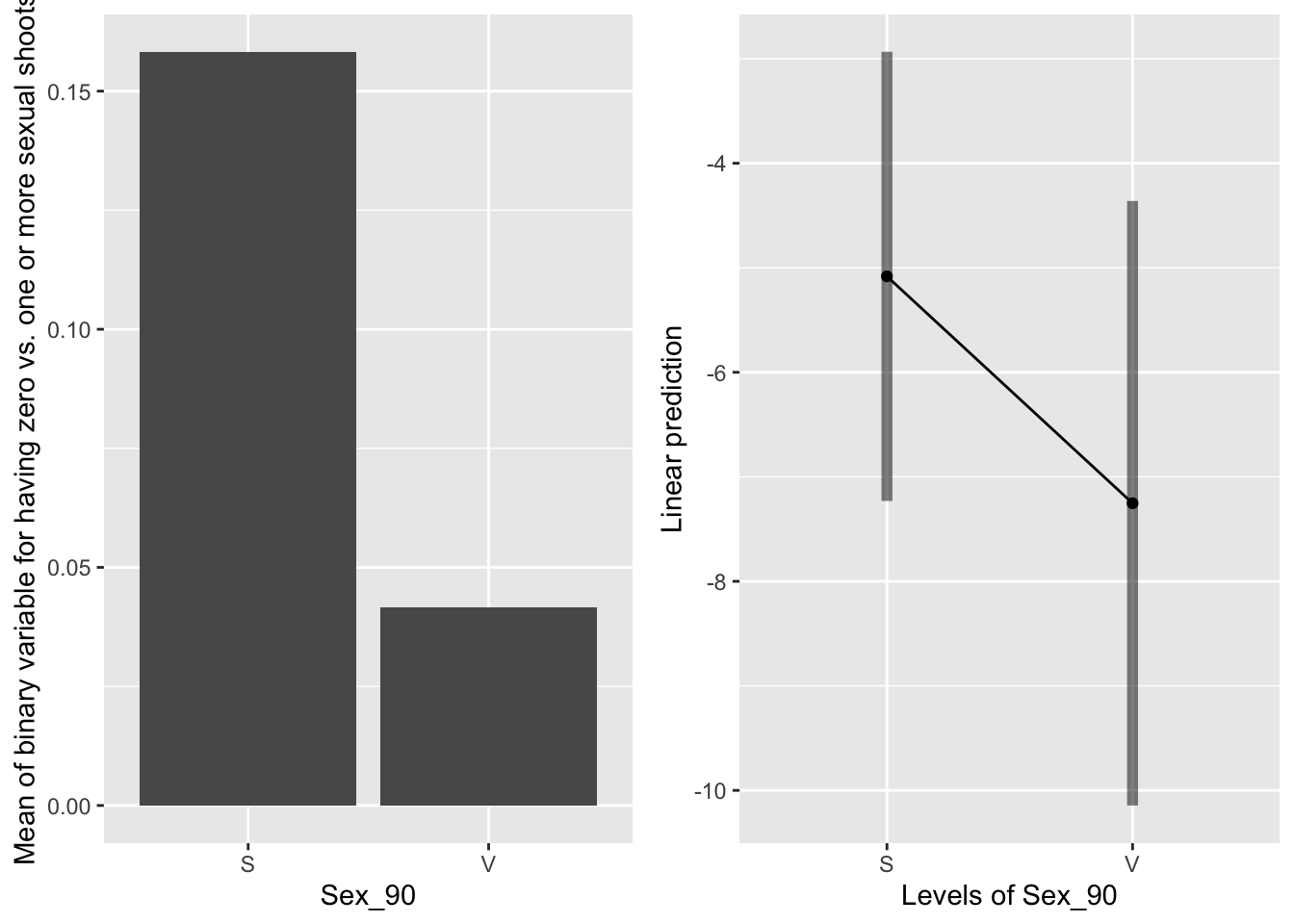
Sexual systems in 1990 are more likely to have a sexual shoot in the back system in 1991.
the main effect of sever
g1 <- ggplot(data=mayappleSexData, aes(x=Sever, y=SexBr)) +
  geom_bar(stat="summary", fun.y = "mean", position = "dodge") +
  ylab("Mean of binary variable for having zero vs. one or more sexual shoots")

emmeans(mod91sexbm, pairwise~Sever, type="response")
## $emmeans
## Sever prob SE df lower.CL upper.CL
## S1 0.025146 0.020383 251 4.99e-03 0.1171
## S2 0.000752 0.001167 251 3.53e-05 0.0158
## S4 0.000475 0.000797 251 1.74e-05 0.0128
##
## Results are averaged over the levels of: Sex_90, Time
## Confidence level used: 0.95
## Intervals are back-transformed from the logit scale
##
## $contrasts
## contrast odds.ratio SE df t.ratio p.value
## S1 / S2 34.30 34.64 251 3.500 0.0016
## S1 / S4 54.32 69.70 251 3.113 0.0058
## S2 / S4 1.58 2.03 251 0.359 0.9315
##
## Results are averaged over the levels of: Sex_90, Time
## P value adjustment: tukey method for comparing a family of 3 estimates
## Tests are performed on the log odds ratio scale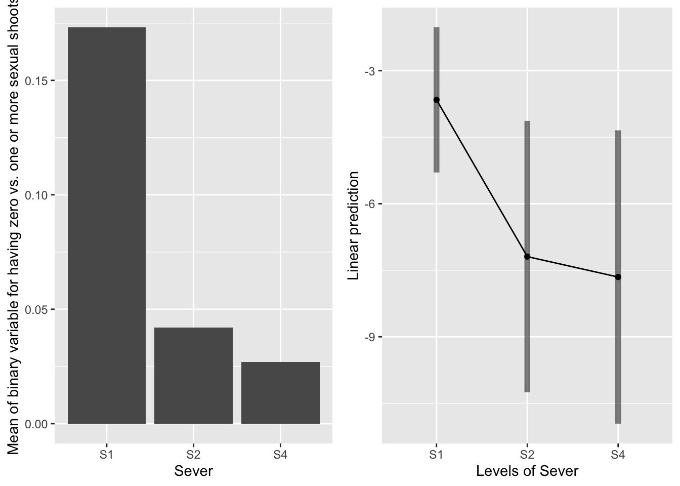 S1 systems are most likely to have sexual shoots in the back. S2 and S4 systems are equivalent, and not likely to have sexual shoots in the back.
the main effect of time
g1 <- ggplot(data=mayappleSexData, aes(x=Time, y=SexBr)) +
  geom_bar(stat="summary", fun.y = "mean", position = "dodge") +
  ylab("Mean of binary variable for having zero vs. one or more sexual shoots")

emmeans(mod91sexbm, pairwise~Time, type="response")
## $emmeans
## Time prob SE df lower.CL upper.CL
## T1 0.000712 0.00121 251 2.50e-05 0.01990
## T2 0.046913 0.03140 251 1.22e-02 0.16404
## T3 0.000263 0.00048 251 7.15e-06 0.00956
##
## Results are averaged over the levels of: Sex_90, Sever
## Confidence level used: 0.95
## Intervals are back-transformed from the logit scale
##
## $contrasts
## contrast odds.ratio SE df t.ratio p.value
## T1 / T2 0.0145 0.02 251 -3.060 0.0069
## T1 / T3 2.7140 4.47 251 0.606 0.8169
## T2 / T3 187.4382 272.25 251 3.603 0.0011
##
## Results are averaged over the levels of: Sex_90, Sever
## P value adjustment: tukey method for comparing a family of 3 estimates
## Tests are performed on the log odds ratio scale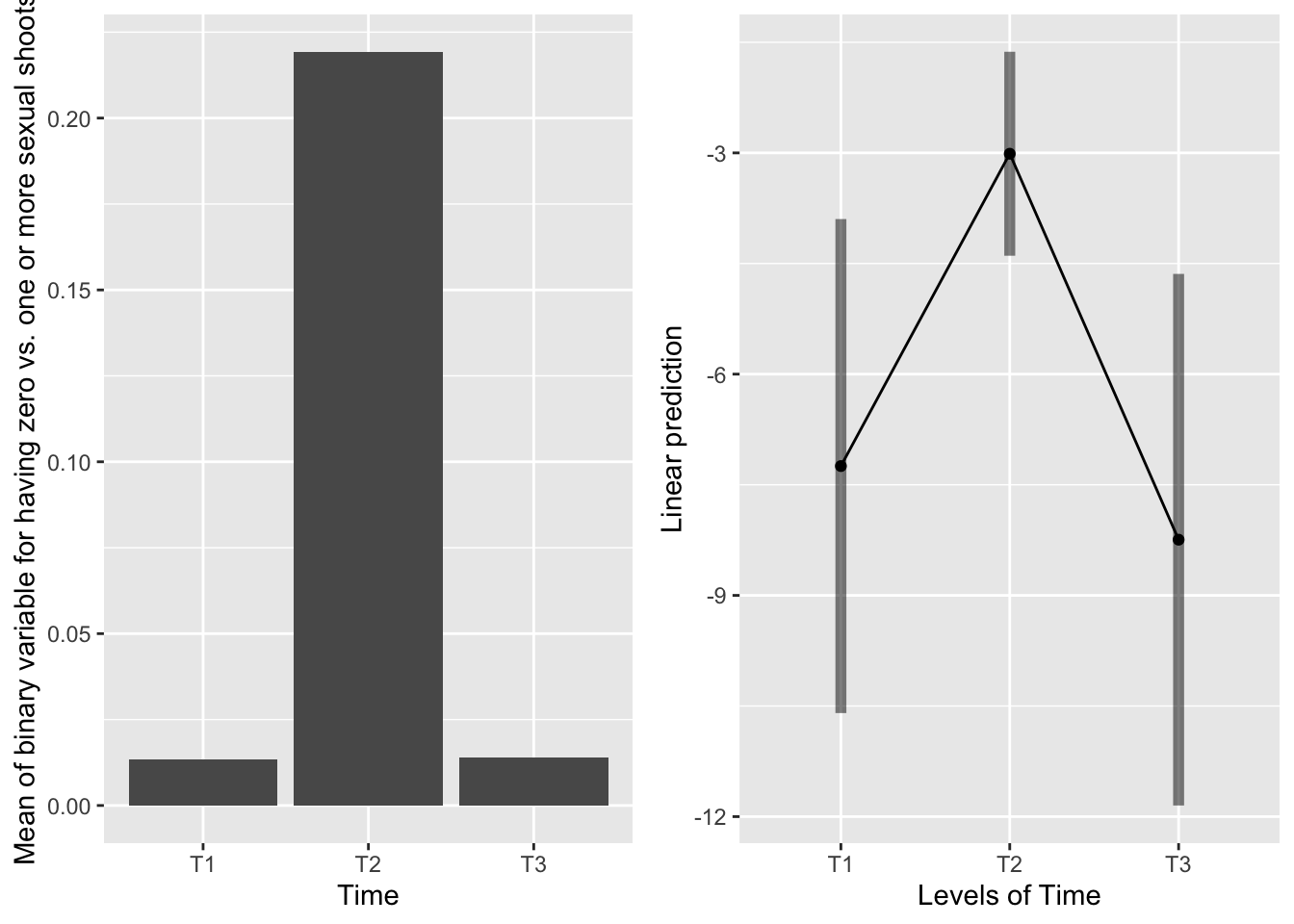
Systems severed at T2 are much more likely to have sexual shoots in the back. T1 and T3 are equivalent, and not likely to have sexual shoots in the back.
the main effect of leaf area
newdat <- expand.grid(Lf_90=seq(min(mayappleSexData$Lf_90,na.rm=TRUE), max(mayappleSexData$Lf_90,na.rm=TRUE),len=100),
                      Sever=c("S1", "S2", "S4"),
                      Time=c("T1", "T2","T3"),
                     Sex_90=c("S","V"),
                     COLONY = mayappleSexData$COLONY)
newdat$brBinary = predict(mod91sexbm, newdata=newdat, type="response",re.form=~0)

ggplot(data=mayappleSexData, aes(x=Lf_90, y=SexBr)) +
  geom_point() + geom_line(data=newdat, aes(x=Lf_90, y=brBinary))+
  facet_wrap(~Sex_90)+
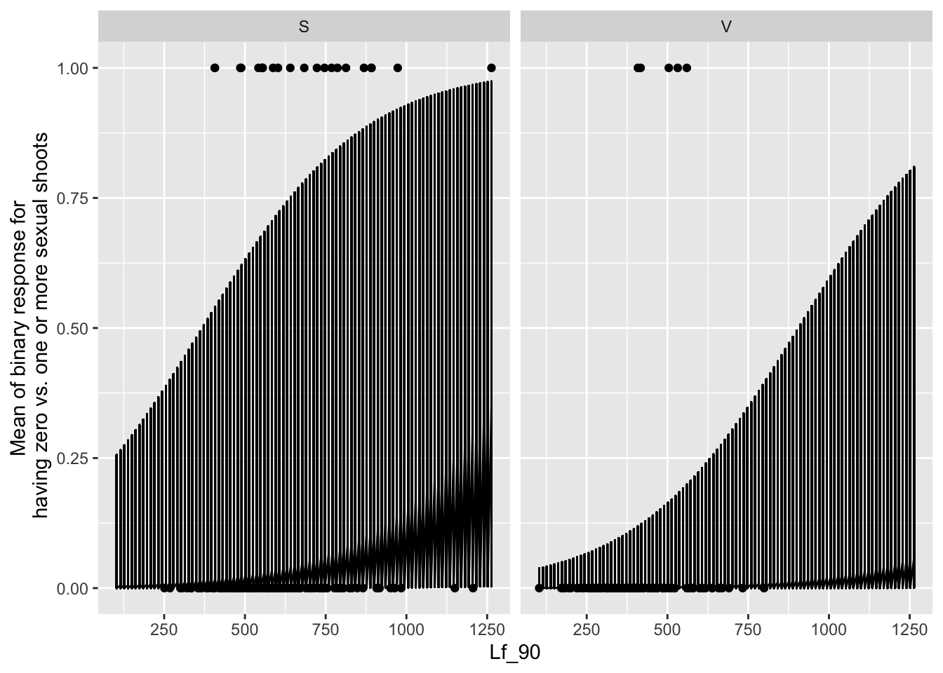
ylab("Mean of binary response for\n having zero vs. one or more sexual shoots") 