2 1990 analyses
2.1 Leaf area in 1990
may<-read.csv("Datasets/mayapple_1990_updated.csv")
##need to make the variables we are working with numeric:
may$Lf_90<-as.numeric(as.character(may$Lf_90))
may$Sen2_90<-as.numeric(as.character(may$Sen2_90))
may$Sen1_90<-as.numeric(as.character(may$Sen1_90))

may<-may %>%
  filter(!is.na(Lf_90))
2.1.1 Visualization
p<- ggplot(data=may) +
  geom_boxplot(aes(x=Sever,y=Lf_90,fill=Time)) +
  facet_wrap(~Sex_90) +
  theme_bw()
print(p)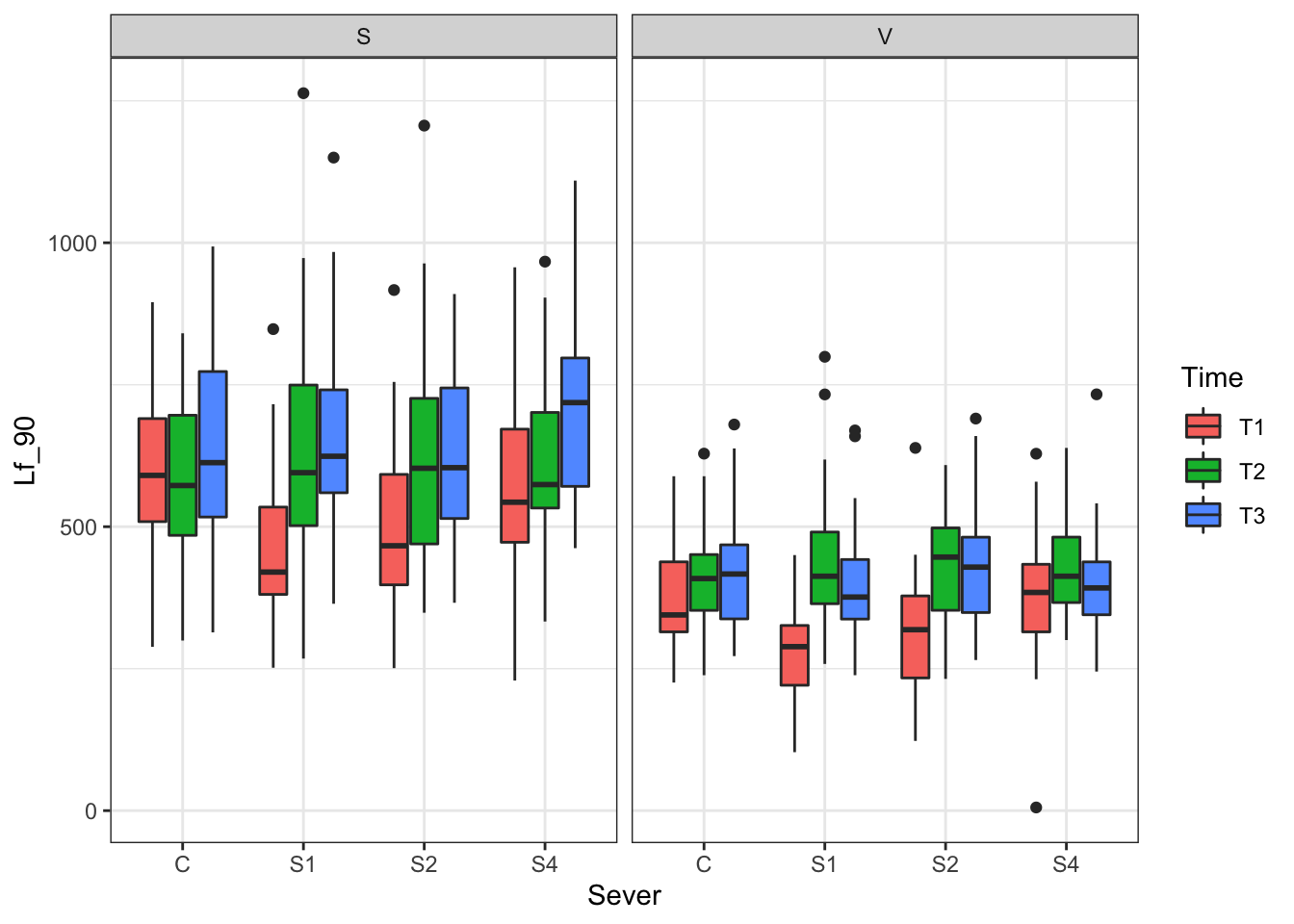
2.1.2 Model specification
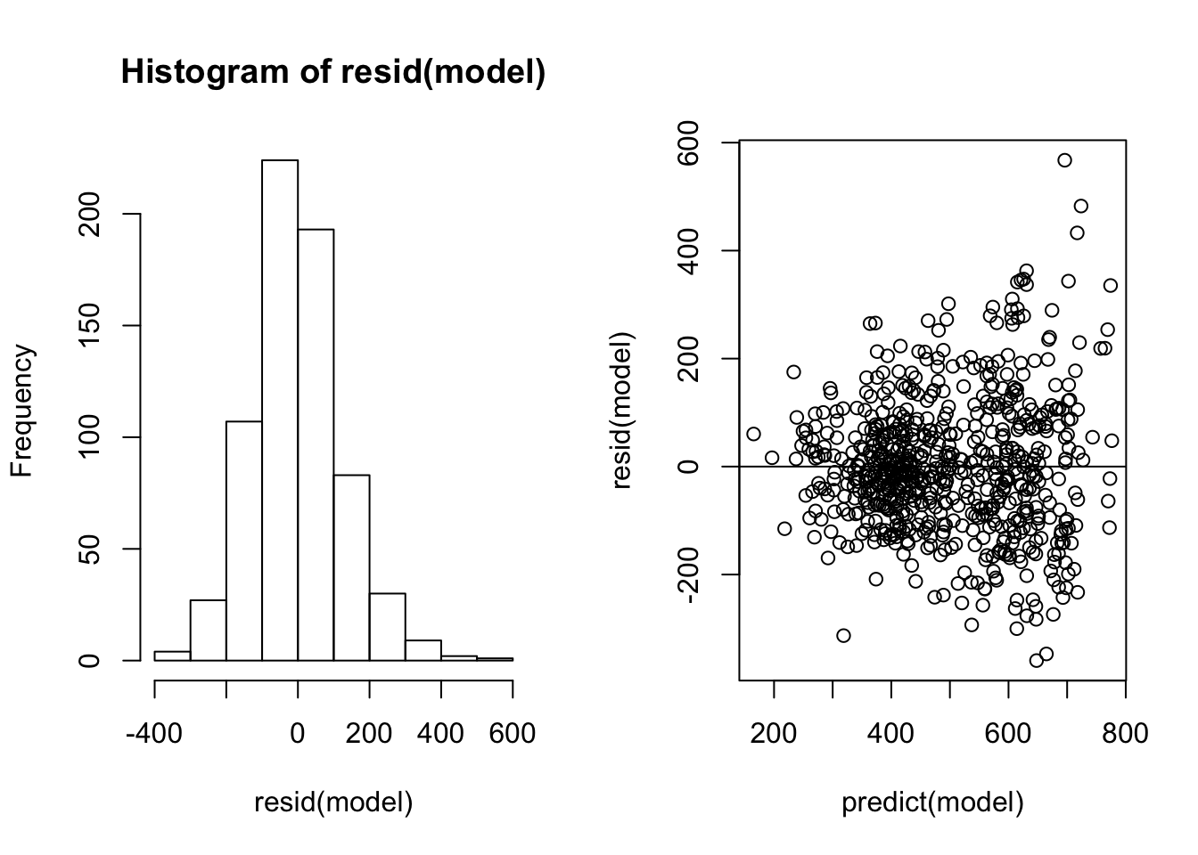
We ran a linear mixed-effects model using lmer. The response was leaf area in 1990. The fixed-effects were sex in 90, severing position, and severing time, and all possible interactions. The random-effects were colony.
We checked and plotted the model residuals:
2.1.3 Model selection
#this is the global model
#MuMIn::getAllTerms(model) #this lets us see how to specify terms in the model

dr<-dredge(model)


tab <- head(dr, n=10) %>% gt() %>%
  fmt_number(columns = vars(`(Intercept)`, logLik, AICc, delta, weight), decimals = 2) %>%
  tab_spanner(label = "Fit information", columns = vars(df, logLik, AICc, delta, weight)) %>%
  tab_spanner(label = "Non-fixed parameters", columns = vars(`(Intercept)`,  Sever, Sex_90, Time,  `Sever:Sex_90`, `Sever:Time`, `Sex_90:Time`, `Sever:Sex_90:Time`)) %>%
  tab_spanner(label = "Fixed parameter", columns = vars(`(Intercept)`)) %>%
    tab_style(style = cell_fill(color = "lightgrey"), locations = cells_body(columns = everything(),rows = delta <= 2)) %>%
  tab_style(style = cell_fill(color = "darkgrey"), locations = cells_body( columns = everything(), rows = 1))

tab %>% gtsave("1990.png", vwidth=1200)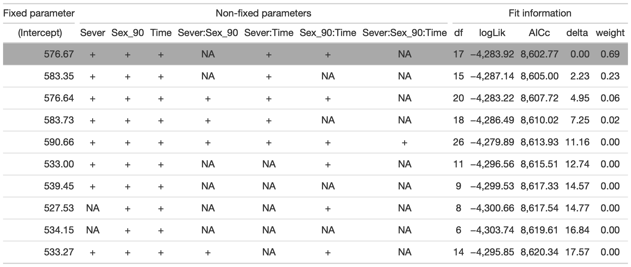
2.1.4 Conclusion
model.bm<-lmer(Lf_90~Sex_90*Time+Sever*Time+(1|COLONY), data=may, na.action = "na.fail", REML=FALSE)The best model includes fixed effects of Sever, Sex_90, Time, the Sever x Time interaction, and the Sex_90 x Time interaction.
2.1.5 Estimated marginal means
We are looking at the estimated marginal means for the significant effects:
The main effect of Sex_90:
g1 <- ggplot(data=may) +
  geom_boxplot(aes(x=Sex_90, y=Lf_90, fill=Sex_90)) +
  theme_bw()
emmeans(model.bm, "Sex_90", type="response")
## Sex_90 emmean SE df lower.CL upper.CL
## S 599 11.7 42.1 576 623
## V 394 11.7 42.7 370 418
##
## Results are averaged over the levels of: Time, Sever
## Degrees-of-freedom method: satterthwaite
## Confidence level used: 0.95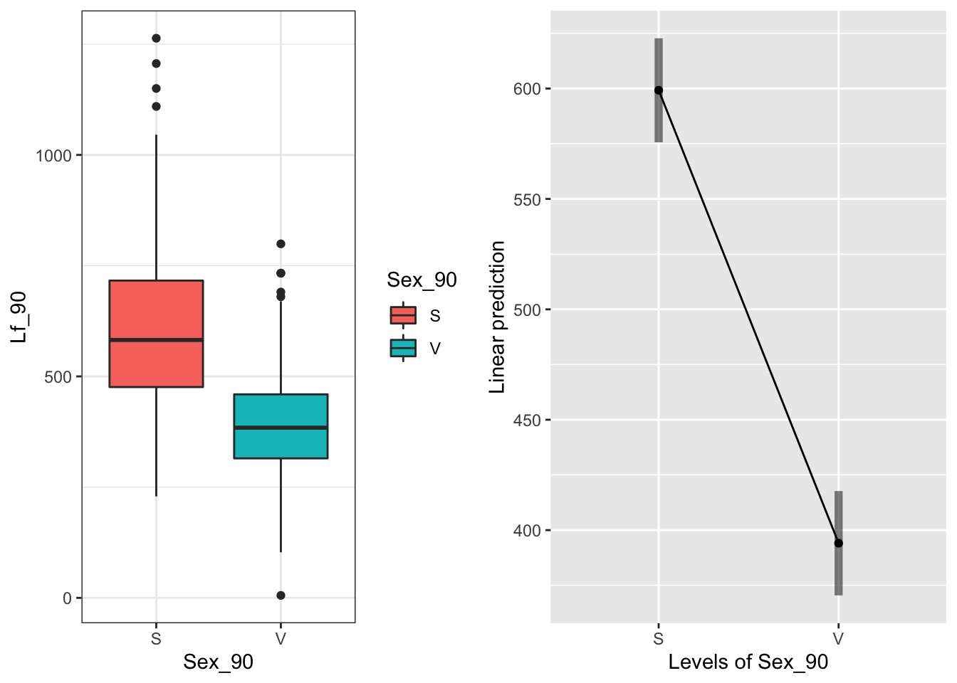 Sexual > Vegetative
The main effect of Sever:
g1 <- ggplot(data=may) +
  geom_boxplot(aes(x=Sever, y=Lf_90, fill=Sever)) +
  theme_bw()

emmeans(model.bm, pairwise~Sever, type="response")
## $emmeans
## Sever emmean SE df lower.CL upper.CL
## C 503 13.6 75.6 476 530
## S1 479 13.5 74.6 452 506
## S2 488 13.6 75.5 461 515
## S4 517 13.7 78.9 490 544
##
## Results are averaged over the levels of: Sex_90, Time
## Degrees-of-freedom method: satterthwaite
## Confidence level used: 0.95
##
## $contrasts
## contrast estimate SE df t.ratio p.value
## C - S1 23.47 13.8 650 1.707 0.3209
## C - S2 14.74 13.8 649 1.070 0.7080
## C - S4 -14.34 13.9 650 -1.028 0.7329
## S1 - S2 -8.73 13.7 650 -0.635 0.9206
## S1 - S4 -37.82 13.9 650 -2.721 0.0337
## S2 - S4 -29.09 13.9 650 -2.086 0.1586
##
## Results are averaged over the levels of: Sex_90, Time
## Degrees-of-freedom method: satterthwaite
## P value adjustment: tukey method for comparing a family of 4 estimates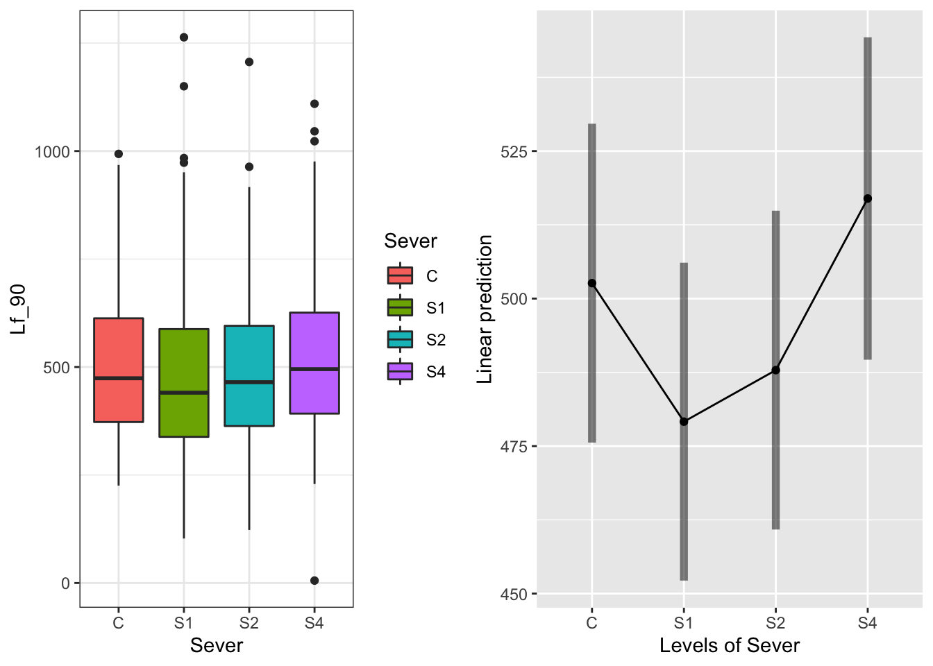 S1 is a bit lower than some of the others, but all of the intervals overlap
The main effect of Time:
g1 <- ggplot(data=may) +
  geom_boxplot(aes(x=Time, y=Lf_90, fill=Time)) +
  theme_bw()

emmeans(model.bm, pairwise~Time, type="response")
## $emmeans
## Time emmean SE df lower.CL upper.CL
## T1 432 12.6 57.6 407 458
## T2 519 12.6 56.7 494 544
## T3 539 12.8 60.5 513 564
##
## Results are averaged over the levels of: Sex_90, Sever
## Degrees-of-freedom method: satterthwaite
## Confidence level used: 0.95
##
## $contrasts
## contrast estimate SE df t.ratio p.value
## T1 - T2 -86.4 11.9 650 -7.283 <.0001
## T1 - T3 -106.3 12.1 652 -8.782 <.0001
## T2 - T3 -19.9 12.0 652 -1.651 0.2252
##
## Results are averaged over the levels of: Sex_90, Sever
## Degrees-of-freedom method: satterthwaite
## P value adjustment: tukey method for comparing a family of 3 estimates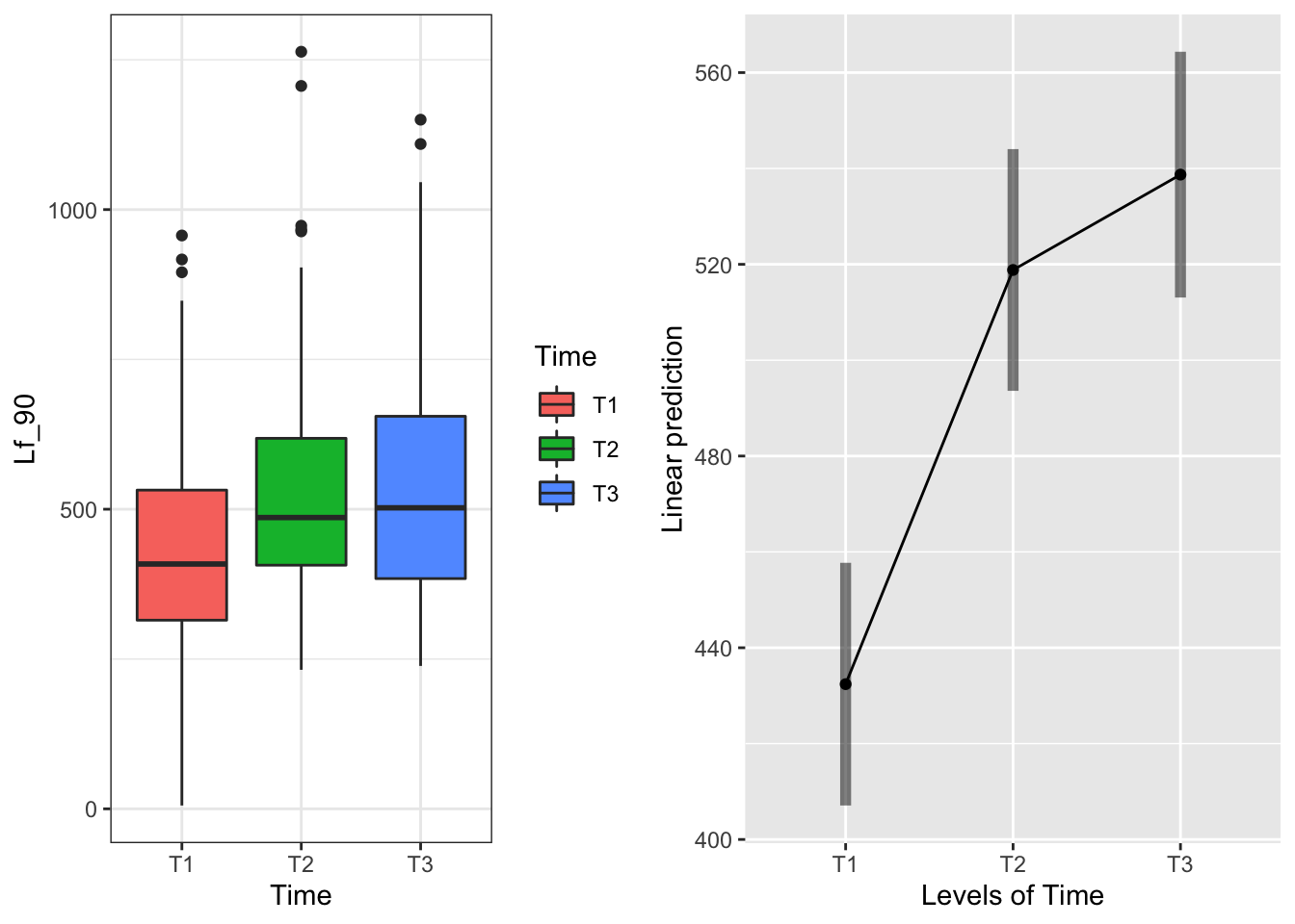 T1 is lower than T2 and T3
The Sex_90 x Time interaction:
g1 <- ggplot(data=may) +
  geom_boxplot(aes(x=Sex_90, y=Lf_90, fill=Time, linetype=Sex_90)) +
  theme_bw()
emmeans(model.bm, pairwise~Time|Sex_90, type="response")
## $emmeans
## Sex_90 = S:
## Time emmean SE df lower.CL upper.CL
## T1 528 15.1 114 498 558
## T2 611 15.0 112 581 641
## T3 659 15.4 122 628 690
##
## Sex_90 = V:
## Time emmean SE df lower.CL upper.CL
## T1 337 15.3 117 307 367
## T2 427 15.2 115 396 457
## T3 418 15.5 123 388 449
##
## Results are averaged over the levels of: Sever
## Degrees-of-freedom method: satterthwaite
## Confidence level used: 0.95
##
## $contrasts
## Sex_90 = S:
## contrast estimate SE df t.ratio p.value
## T1 - T2 -83.56 16.7 649 -5.017 <.0001
## T1 - T3 -131.37 17.0 650 -7.723 <.0001
## T2 - T3 -47.82 16.9 650 -2.822 0.0136
##
## Sex_90 = V:
## contrast estimate SE df t.ratio p.value
## T1 - T2 -89.27 16.9 650 -5.283 <.0001
## T1 - T3 -81.24 17.2 651 -4.732 <.0001
## T2 - T3 8.03 17.1 651 0.470 0.8853
##
## Results are averaged over the levels of: Sever
## Degrees-of-freedom method: satterthwaite
## P value adjustment: tukey method for comparing a family of 3 estimates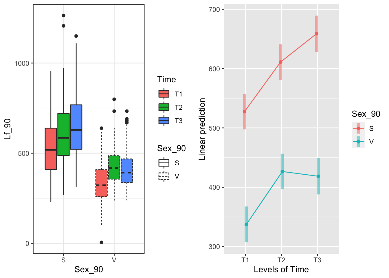 For each sex, there are bigger differences between T1 and T2,T3; T2 and T3 are more similar to each other
## Cannot use mode = "kenward-roger" because *pbkrtest* package is not installed## $emmeans
## Time = T1:
## Sex_90 emmean SE df lower.CL upper.CL
## S 528 15.1 114 498 558
## V 337 15.3 117 307 367
##
## Time = T2:
## Sex_90 emmean SE df lower.CL upper.CL
## S 611 15.0 112 581 641
## V 427 15.2 115 396 457
##
## Time = T3:
## Sex_90 emmean SE df lower.CL upper.CL
## S 659 15.4 122 628 690
## V 418 15.5 123 388 449
##
## Results are averaged over the levels of: Sever
## Degrees-of-freedom method: satterthwaite
## Confidence level used: 0.95
##
## $contrasts
## Time = T1:
## contrast estimate SE df t.ratio p.value
## S - V 190 16.8 649 11.298 <.0001
##
## Time = T2:
## contrast estimate SE df t.ratio p.value
## S - V 185 16.7 649 11.058 <.0001
##
## Time = T3:
## contrast estimate SE df t.ratio p.value
## S - V 240 17.3 650 13.918 <.0001
##
## Results are averaged over the levels of: Sever
## Degrees-of-freedom method: satterthwaiteLooking at this the other way, the area generally increases with later severing in both sexes, but T2 and T3 are basically the same for vegetative
The Sever x Time interaction:
g1<-ggplot(data=may) +
  geom_boxplot(aes(x=Sever, y=Lf_90, fill=Time)) +
  theme_bw()
emmeans(model.bm, pairwise~Time|Sever, type="response")
## $emmeans
## Sever = C:
## Time emmean SE df lower.CL upper.CL
## T1 481 19.6 268 443 520
## T2 496 19.1 248 458 533
## T3 531 19.3 257 493 569
##
## Sever = S1:
## Time emmean SE df lower.CL upper.CL
## T1 372 19.1 248 334 409
## T2 537 19.2 252 499 575
## T3 529 19.5 262 490 567
##
## Sever = S2:
## Time emmean SE df lower.CL upper.CL
## T1 406 19.3 257 368 444
## T2 524 19.2 252 486 561
## T3 534 19.5 262 495 572
##
## Sever = S4:
## Time emmean SE df lower.CL upper.CL
## T1 470 19.2 252 432 508
## T2 519 19.2 252 482 557
## T3 561 20.6 303 521 602
##
## Results are averaged over the levels of: Sex_90
## Degrees-of-freedom method: satterthwaite
## Confidence level used: 0.95
##
## $contrasts
## Sever = C:
## contrast estimate SE df t.ratio p.value
## T1 - T2 -14.01 23.9 650 -0.586 0.8276
## T1 - T3 -49.34 24.1 650 -2.046 0.1021
## T2 - T3 -35.34 23.7 650 -1.492 0.2953
##
## Sever = S1:
## contrast estimate SE df t.ratio p.value
## T1 - T2 -165.05 23.6 649 -7.007 <.0001
## T1 - T3 -156.89 23.8 650 -6.597 <.0001
## T2 - T3 8.16 23.9 650 0.342 0.9377
##
## Sever = S2:
## contrast estimate SE df t.ratio p.value
## T1 - T2 -117.25 23.8 650 -4.932 <.0001
## T1 - T3 -127.60 24.0 650 -5.316 <.0001
## T2 - T3 -10.35 23.9 650 -0.433 0.9018
##
## Sever = S4:
## contrast estimate SE df t.ratio p.value
## T1 - T2 -49.36 23.7 649 -2.086 0.0935
## T1 - T3 -91.40 24.8 651 -3.690 0.0007
## T2 - T3 -42.04 24.8 651 -1.697 0.2072
##
## Results are averaged over the levels of: Sex_90
## Degrees-of-freedom method: satterthwaite
## P value adjustment: tukey method for comparing a family of 3 estimates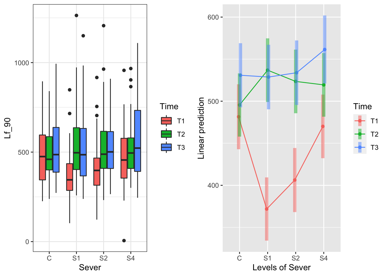 For controls, timing of severing doesn’t matter
For S1 and also S2, severing early (T1) yields lower leaf area than severing later (T2 or T3)
For S4, severing earliest (T1) yields lower leaf area than severing latest (T3)
For controls, timing of severing doesn’t matter
For S1 and also S2, severing early (T1) yields lower leaf area than severing later (T2 or T3)
For S4, severing earliest (T1) yields lower leaf area than severing latest (T3)
Making plots for the MS:
##This is using the emmeans

g1 <- emmip(model.bm, Sex_90  ~ Time  ,CIs = TRUE)+ ggtitle("The sex x time interaction")+
  theme_bw()+theme(plot.title = element_text(face="italic"))+theme(panel.grid.major = element_blank(), panel.grid.minor = element_blank())
## Cannot use mode = "kenward-roger" because *pbkrtest* package is not installedg2 <- emmip(model.bm, ~ Time ,CIs = TRUE) + ggtitle("The main effect of time") +
theme_bw()+theme(plot.title = element_text(face="italic"))+theme(panel.grid.major = element_blank(), panel.grid.minor = element_blank())## Cannot use mode = "kenward-roger" because *pbkrtest* package is not installed## NOTE: Results may be misleading due to involvement in interactionsg3 <- emmip(model.bm, ~ Sex_90 ,CIs = TRUE) +ggtitle("The main effect of sex")+
theme_bw()+theme(plot.title = element_text(face="italic"))+theme(panel.grid.major = element_blank(), panel.grid.minor = element_blank())## Cannot use mode = "kenward-roger" because *pbkrtest* package is not installed
## NOTE: Results may be misleading due to involvement in interactionsg4 <- emmip(model.bm, Sever ~ Time ,CIs = TRUE)+ggtitle("The sever x time interaction")+
theme_bw()+theme(plot.title = element_text(face="italic"))+theme(panel.grid.major = element_blank(), panel.grid.minor = element_blank())## Cannot use mode = "kenward-roger" because *pbkrtest* package is not installedg5 <- emmip(model.bm, ~ Sever ,CIs = TRUE) +ggtitle("The main effect of sever")+
theme_bw()+theme(plot.title = element_text(face="italic"))+theme(panel.grid.major = element_blank(), panel.grid.minor = element_blank())## Cannot use mode = "kenward-roger" because *pbkrtest* package is not installed
## NOTE: Results may be misleading due to involvement in interactions##This is using the raw values
g1 <- ggplot(data=may) +
geom_boxplot(aes(x=Sex_90, y=Lf_90, fill=Time, linetype=Sex_90)) + scale_linetype(guide=FALSE) +scale_fill_discrete(guide=FALSE)+
ylab("Leaf area in 1990")+ xlab("Sex in 1990")+ ggtitle("The sex x time interaction")+
theme_bw()+theme(plot.title = element_text(face="italic"))+theme(panel.grid.major = element_blank(), panel.grid.minor = element_blank())
g2 <- ggplot(data=may) +
geom_boxplot(aes(x=Time, y=Lf_90, fill=Time)) +ylab("")+ ggtitle("The main effect of time")+
theme_bw()+theme(plot.title = element_text(face="italic"))+theme(panel.grid.major = element_blank(), panel.grid.minor = element_blank())
g3 <- ggplot(data=may) +
geom_boxplot(aes(x=Sex_90, y=Lf_90, linetype=Sex_90)) + ylab("")+ xlab("Sex in 1990")+
ggtitle("The main effect of sex")+
theme_bw()+theme(plot.title = element_text(face="italic"))+theme(panel.grid.major = element_blank(), panel.grid.minor = element_blank())
g4 <- ggplot(data=may) +
geom_boxplot(aes(x=Sever, y=Lf_90, fill=Time, color=Sever)) + scale_color_discrete(guide=FALSE) +scale_fill_discrete(guide=FALSE)+
ylab("Leaf area in 1990")+ xlab("Severing location")+ggtitle("The sever x time interaction")+
theme_bw()+theme(plot.title = element_text(face="italic"))+theme(panel.grid.major = element_blank(), panel.grid.minor = element_blank())
g5 <- ggplot(data=may) +
geom_boxplot(aes(x=Sever, y=Lf_90, color=Sever)) + ylab("")+ xlab("Severing location")+ ggtitle("The main effect of sever")+
theme_bw()+theme(plot.title = element_text(face="italic")) +theme(panel.grid.major = element_blank(), panel.grid.minor = element_blank())
#lay <- rbind(c(1,2),
# c(NA,3),
# c(4,5))
#gridExtra::grid.arrange(
# g1, g2, g3,g4, g5,
# layout_matrix = lay)
library("cowplot")##
## ********************************************************## Note: As of version 1.0.0, cowplot does not change the## default ggplot2 theme anymore. To recover the previous## behavior, execute:
## theme_set(theme_cowplot())## ********************************************************##
## Attaching package: 'cowplot'## The following object is masked from 'package:ggeffects':
##
## get_titleggdraw()+
draw_plot(g1, x=0, y=0.5, width = .67, height = .5)+
draw_plot(g3, x=0.67, y=0.67, width = 0.33, height = 0.33 ) +
draw_plot(g2, x=0.67, y=0.33, width = 0.33, height = 0.33) +
draw_plot(g4, x=0, y=0, width = .67, height = .5) +
draw_plot(g5, x=0.67, y=0,width = 0.33, height = 0.33 )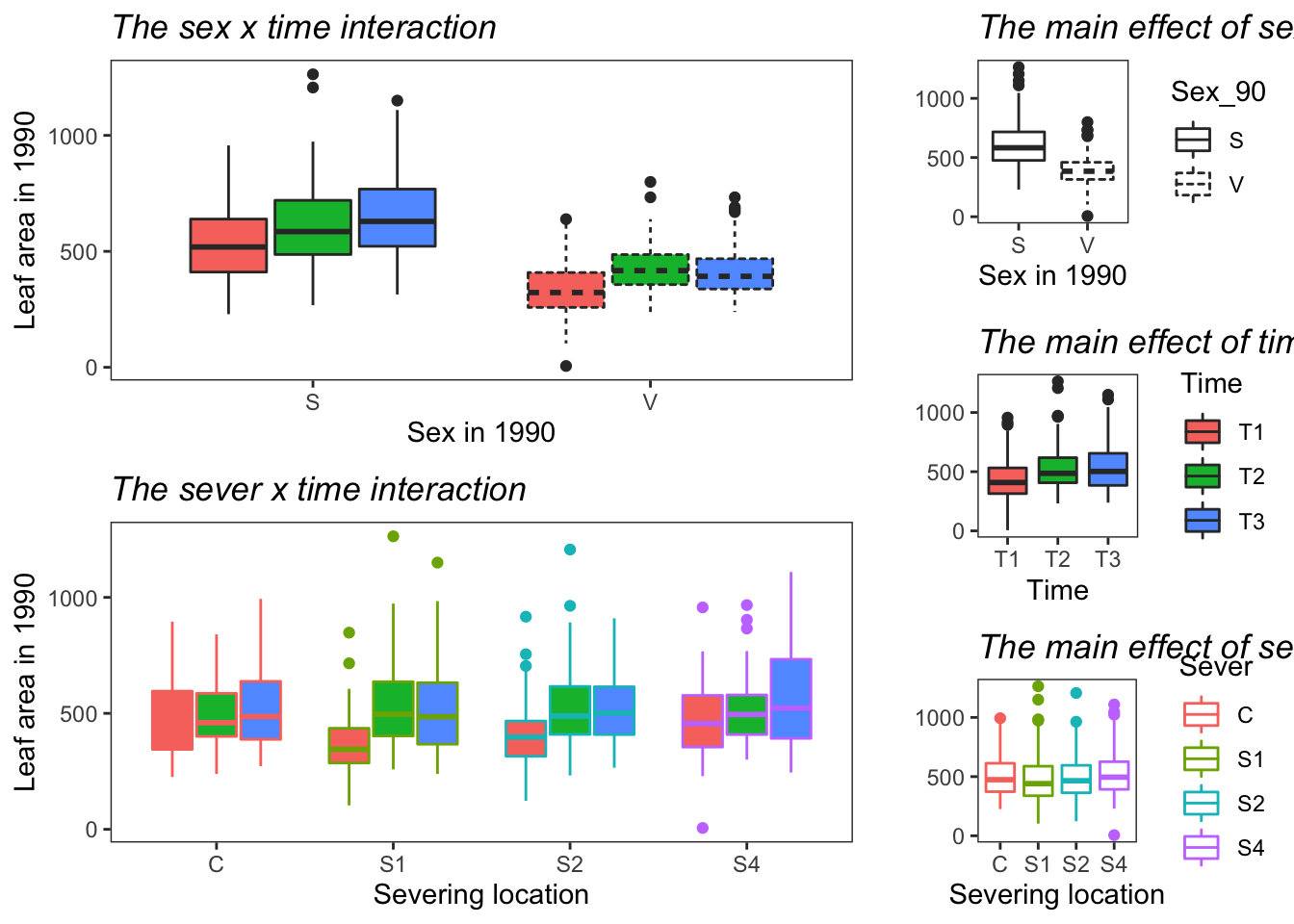
2.2 Senescence
The second question we addressed was: do sex, severing treatment, severing time, or any interactions affect time of senescence in 1990? Here’s a summary of that data
2.2.1 Visualization
p<- ggplot(data=may) +
  geom_boxplot(aes(x=Sever,y=Sen2_90,fill=Time)) +
  facet_wrap(~Sex_90) +
  theme_bw()
print(p)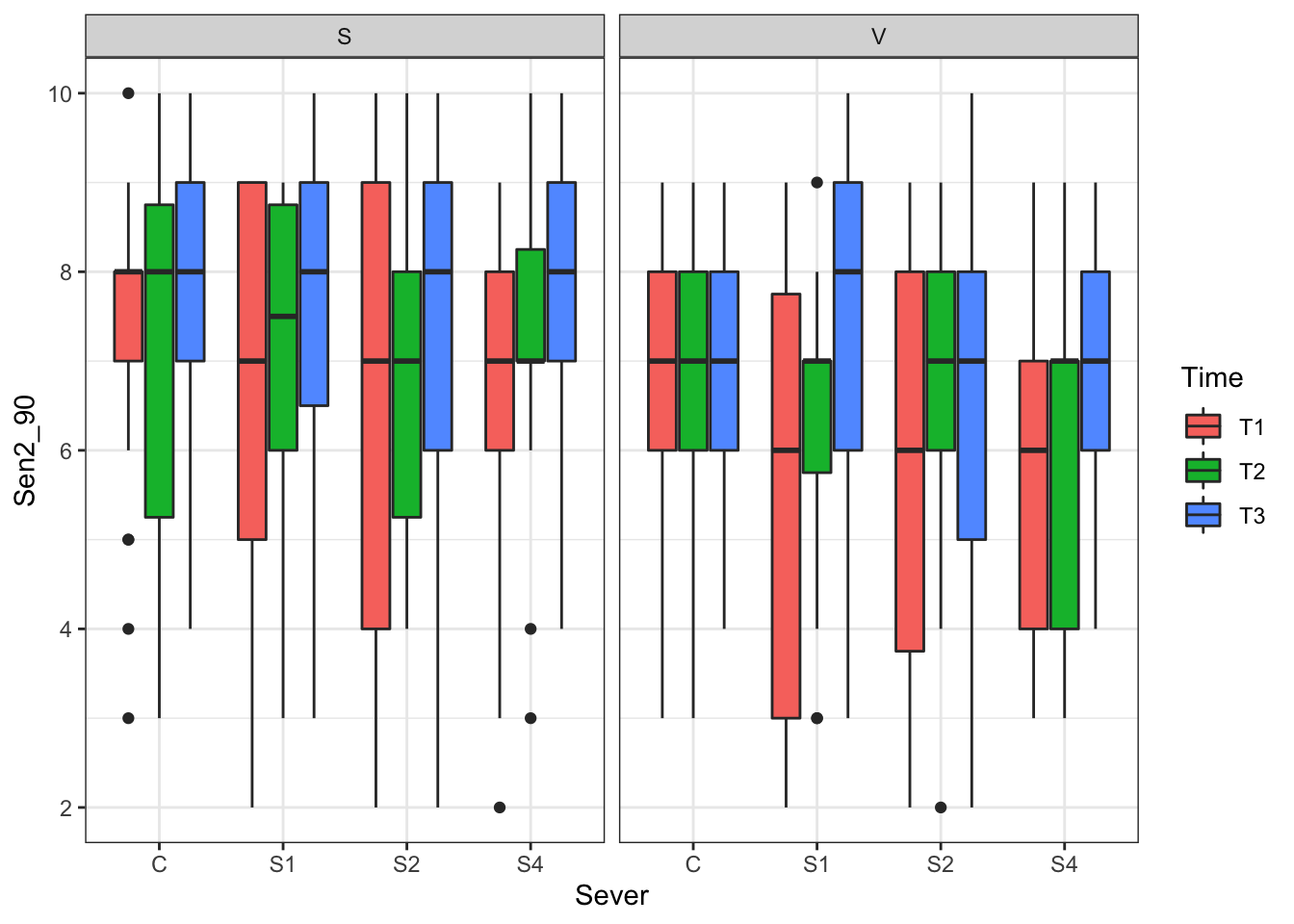
2.2.2 Pilot analysis with the controls
First, we wanted to look at whether sex and leaf area have any effect on senescence in the control plants.
#this is just the control plants
may.c<-may[which(may$Sever=="C"),]
#here is that model:
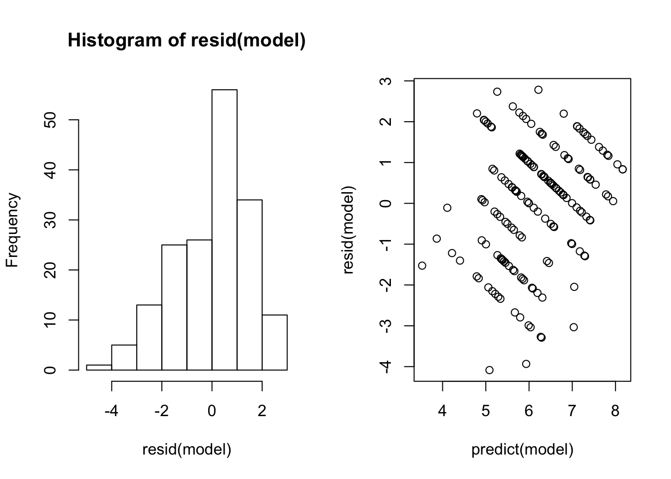
model<-lmer(Sen1_90~Sex_90*Lf_90+(1|COLONY), data=may.c)
summary(model)## Linear mixed model fit by REML. t-tests use Satterthwaite's method [
## lmerModLmerTest]
## Formula: Sen1_90 ~ Sex_90 * Lf_90 + (1 | COLONY)
## Data: may.c
##
## REML criterion at convergence: 694.4
##
## Scaled residuals:
## Min 1Q Median 3Q Max
## -2.6244 -0.6998 0.1711 0.6648 1.7879
##
## Random effects:
## Groups Name Variance Std.Dev.
## COLONY (Intercept) 1.056 1.028
## Residual 2.422 1.556
## Number of obs: 171, groups: COLONY, 30
##
## Fixed effects:
## Estimate Std. Error df t value Pr(>|t|)
## (Intercept) 5.598e+00 7.542e-01 1.666e+02 7.422 5.62e-12 ***
## Sex_90V -1.723e-01 1.077e+00 1.542e+02 -0.160 0.873
## Lf_90 1.364e-03 1.177e-03 1.568e+02 1.159 0.248
## Sex_90V:Lf_90 -3.776e-04 2.282e-03 1.554e+02 -0.165 0.869
## ---
## Signif. codes: 0 '***' 0.001 '**' 0.01 '*' 0.05 '.' 0.1 ' ' 1
##
## Correlation of Fixed Effects:
## (Intr) Sx_90V Lf_90
## Sex_90V -0.640
## Lf_90 -0.943 0.641
## Sx_90V:L_90 0.466 -0.955 -0.493Here are the residuals from that model
And here is the summary of data from just the control plants

## Type III Analysis of Variance Table with Satterthwaite's method
##               Sum Sq Mean Sq NumDF  DenDF F value Pr(>F)
## Sex_90       0.06198 0.06198     1 154.17  0.0256 0.8731
## Lf_90        2.45628 2.45628     1 160.12  1.0140 0.3155
## Sex_90:Lf_90 0.06634 0.06634 1 155.39 0.0274 0.8688Conclusion: while the sexes occupy different ranges of leaf areas, there isn’t a relationship between leaf area and sensecence time overall
2.2.3 Main model specification
mod90s<-lmer(Sen2_90~Sex_90*Sever*Time+(1|COLONY), data=may)
mod90s.<-lmer(Sen2_90~ Sex_90*Sever + Sex_90*Time + Sever*Time + (1|COLONY), data = may) #removing the three-way interaction
mod90s.a<-lmer(Sen2_90~  Sex_90*Time + Sever*Time + (1|COLONY), data = may) #removing the Sex x Sever interaction
mod90s.b<-lmer(Sen2_90~ Sex_90*Sever +  Sever*Time + (1|COLONY), data = may) #removing the Sex x Time interaction
mod90s.c<-lmer(Sen2_90~ Sex_90*Sever + Sex_90*Time +  (1|COLONY), data = may) #removing the Sever x Time interaction
mod90s.d<-lmer(Sen2_90~ Sex_90*Sever + Time +  (1|COLONY), data = may) #only the Sex x Sever interaction
mod90s.e<-lmer(Sen2_90~ Sex_90*Time + Sever +  (1|COLONY), data = may) #only the Sex x Time interaction
mod90s.f<-lmer(Sen2_90~ Sex_90 +  Sever*Time + (1|COLONY), data = may) #only the Sever x Time interaction
mod90s.g<-lmer(Sen2_90~ Sex_90 +  Sever+Time + (1|COLONY), data = may) #no interactions
mod90s.h<-lmer(Sen2_90~   Sever+Time + (1|COLONY), data = may) #Sever and Time
mod90s.i<-lmer(Sen2_90~   Sex_90+Time + (1|COLONY), data = may) #Sex and Time
mod90s.j<-lmer(Sen2_90~   Sex_90+Sever + (1|COLONY), data = may) #Sex and Sever
mod90s.k<-lmer(Sen2_90~   Sever + (1|COLONY), data = may) #Sever
mod90s.l<-lmer(Sen2_90~   Time + (1|COLONY), data = may) #Time
mod90s.m<-lmer(Sen2_90~   Sex_90 + (1|COLONY), data = may) #Sex
mod90s.n<-lmer(Sen2_90~    (1|COLONY), data = may) #random effect only; null model
2.2.4 Model results
| Model name | Main effects | AIC | vs model, what is this testing | Chi-sq | P |
|---|---|---|---|---|---|
| mod90s | full model | 2710.9 | mod90s., sig of the three-way int. | 5.3027 | 0.5056 |
| mod90s. | all two-ways | 2704.2 | mod90s.a, sig of the sex x sever int. | 1.3734 | 0.7118 |
| mod90s.b, sig of the sex x time int. | 2.1507 | 0.3412 | |||
| mod90s.c, sig of the sever x time ints | 4.9642 | 0.5484 | |||
| mod90s.a | sex x time and sever x time ints | 2699.6 | mod90s.e, sig of the sever x time | 4.9416 | 0.5513 |
| mod90s.f, sig of the sex x time | 2.2096 | 0.3313 | |||
| mod90s.b | sex x sever and sever x time ints | 2702.4 | mod90s.d, sig of the sever x time int | 4.9835 | 0.5459 |
| mod90s.f, sig of the sex x sever int | 1.4324 | 0.698 | |||
| mod90s.c | sex x sever and sex x time ints | 2697.2 | mod90s.e, sig of the sex x sever int | 1.3508 | 0.7171 |
| mod90s.d, sig of the sex x tim int | 2.1699 | 0.3379 | |||
| mod90s.d | sex x sever int, and time | 2695.4 | mod90s.g, sig of the sex x sever int | 1.406 | 0.7267 |
| mod90s.e | sex x time int, and sever | 2692.6 | mod90s.g, sig of the sex x time int | 2.2252 | 0.3287 |
| mod90s.f | sever x time int, and sex | 2697.8 | mod90s.g, sig of the sever x time int | 4.9571 | 0.5493 |
| mod90s.g | no interactions, all fixed effects | 2690.8 | mod90s.h, sig of sex | 33.906 | 5.754e-09 *** |
| mod90s.i, sig of sever | 5.2654 | 0.1534 | |||
| mod90s.j, sig of time | 36.499 | 1.187e-08 *** | |||
| mod90s.h | sever and time | 2722.7 | mod90s.l, sig of sever | 5.0036 | 0.1715 |
| mod90s.k, sig of time | 34.358 | 3.461e-08 *** | |||
| mod90s.i | sex and time | 2690.1 | mod90s.m, sig of time | 78.992 | 1.081e-08 *** |
| mod90s.l, sig of sex | 33.654 | 6.583e-09 *** | |||
| mod90s.j | sex and sever | 2723.3 | mod90s.k, sig of sex | 31.776 | 1.73e-08 *** |
| mod90s.m, sig of sever | 5.4516 | 0.1416 | |||
| mod90s.k | sever | 2753.1 | mod90s.n, sig of sever | 5.1944 | 0.1581 |
| mod90s.l | time | 2721.7 | mod90s.n, sig of time | 34.549 | 3.146e-08 *** |
| mod90s.m | sex | 2722.7 | mod90s.n, sig of sex | 31.519 | 1.975e-08 *** |
| mod90s.n | random effect only | 2752.3 |
2.2.5 Conclusions
The best model has fixed effects of sex and time.
2.2.6 Estimated marginal means
For Sex:
g1<- ggplot(data=may) +
 geom_boxplot(aes(x=Sex_90, y=Sen2_90, fill=Sex_90)) +
  theme_bw()
emmeans(mod90s.g, "Sex_90", type="response")
## Sex_90 emmean SE df lower.CL upper.CL
## S 7.15 0.184 37.1 6.78 7.52
## V 6.42 0.184 37.4 6.05 6.80
##
## Results are averaged over the levels of: Sever, Time
## Degrees-of-freedom method: satterthwaite
## Confidence level used: 0.95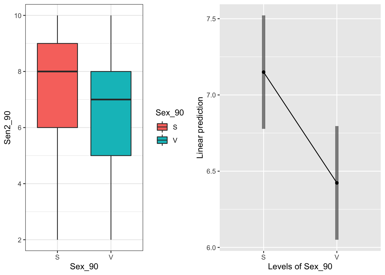 Sexual systems senesce later
For Time:
g1<-ggplot(data=may) +
 geom_boxplot(aes(x=Time, y=Sen2_90, fill=Time)) +
  theme_bw()
emmeans(mod90s.g, "Time", type="response")
## Time emmean SE df lower.CL upper.CL
## T1 6.31 0.194 46.1 5.92 6.70
## T2 6.79 0.193 45.6 6.40 7.18
## T3 7.26 0.196 48.1 6.86 7.65
##
## Results are averaged over the levels of: Sex_90, Sever
## Degrees-of-freedom method: satterthwaite
## Confidence level used: 0.95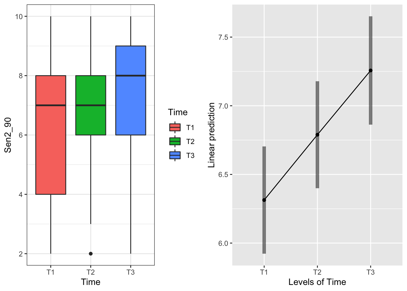 Intervals are overlapping but T3 systems senesce later
2.3 Fruit Production
We wanted to analyze fruit production but cannot because all of the sexual shoots failed to fruit in 1990.