3 1991 front shoot analyses
3.1 Survival
This analysis uses all systems observed in 1991.
3.1.1 Data & visualization
Read in data
# set na.strings="." to recode '.' to NA
mayappleDatasetFull<-readxl::read_excel("Datasets/mayapple_1990_updated.xlsx", na=".")
Select variables from the front of the system. Also filtering out rows that don’t have a leaf area record in 1990. We need to do this in order to be able to compare models from model set A (which don’t include leaf area, and so wouldn’t naturally be affected by the missing data) with models from model set B (which do include leaf area and would be affected by the missing data). In other words, removing these rows means that model set A and model set B will run using the exact same dataset, which is necessary in order for us to compare the models.
# select variables for analysis and filter out rows that don't have a leaf area recorded in 1990
mayappleData <- mayappleDatasetFull %>%
  dplyr::select(COLONY,Lf_90,brnoF_91,Sex_90,Sever,Time,SexF1_91,SexF2_91,SexF3_91,LfFtot_91) %>%
  filter(!is.na(Lf_90))
Creating the dead/alive binary and visualizing:
# create binary variable for plants that are dead/have no branches (0) or have 1 or more branches (1)
# append new variable to the dataframe
mayappleData<- mayappleData %>%
  dplyr::mutate(deadAliveBinary=ifelse(brnoF_91>0,1,0))

# create a plot showing the mean of the binary response variable in each category
# interpretation for values = 0, all responses were 0 in that category (all plants dead)
# interpretation for values = 1, all responses were 1 in that category (all plants alive)

ggplot(data=mayappleData, aes(x=Sever, y=deadAliveBinary, fill = Time)) +
  stat_summary(fun = mean, geom = "bar",position="dodge") +
    stat_summary(fun.data = mean_se, geom = "errorbar", position="dodge")+
  facet_wrap(~Sex_90) +
  ylab("Mean of binary response for\n dead/alive") +
  scale_fill_brewer(palette="Set1")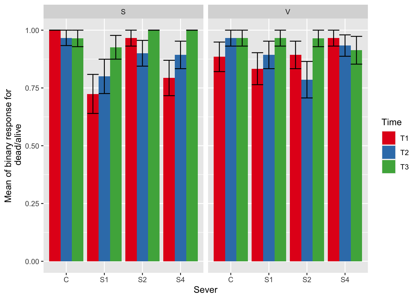
From this plot, we can see that several of the categories have no deaths. This is likely why the three-way interaction doesn’t run for this response variable (see below).
3.1.2 Model selection with leaf area
mod91sur0l<-glmmTMB(deadAliveBinary~ Sex_90*Sever + Sex_90*Time + Sever*Time + Lf_90 + (1|COLONY), data = mayappleData,
                family="binomial")
#this is the global model
#MuMIn::getAllTerms(mod91sur0l) #this lets us see how to specify terms in the model

dr<-dredge(mod91sur0l, fixed=~cond(Lf_90))

tab <- head(dr, n=10) %>% gt() %>% cols_hide(columns=vars(`disp((Int))`)) %>%
  cols_label(`cond((Int))`="(Intercept)", `cond(Lf_90)`="Lf_90", `cond(Sever)`="Sever", `cond(Sex_90)`="Sex_90", `cond(Time)`="Time", `cond(Sever:Sex_90)`="Sever:Sex_90", `cond(Sever:Time)`="Sever:Time", `cond(Sex_90:Time)`= "Sex_90:Time") %>%
  fmt_number(columns = vars(`cond((Int))`, logLik, AICc, delta, weight), decimals = 2) %>%
  fmt_number(columns = vars(`cond(Lf_90)`), decimals = 4) %>%
  tab_spanner(label = "Fit information", columns = vars(df, logLik, AICc, delta, weight)) %>%
  tab_spanner(label = "Non-fixed parameters", columns = vars(`cond((Int))`,  `cond(Lf_90)`, `cond(Sever)`, `cond(Sex_90)`, `cond(Time)`, `cond(Sever:Sex_90)`, `cond(Sever:Time)`, `cond(Sex_90:Time)`)) %>%
  tab_spanner(label = "Fixed parameters", columns = vars(`cond((Int))`,  `cond(Lf_90)`)) %>%
    tab_style(style = cell_fill(color = "lightgrey"), locations = cells_body(columns = everything(),rows = delta <= 2)) %>%
  tab_style(style = cell_fill(color = "darkgrey"), locations = cells_body( columns = everything(), rows = 2))


tab %>% gtsave("front_91_sur_a.png", vwidth=1200) 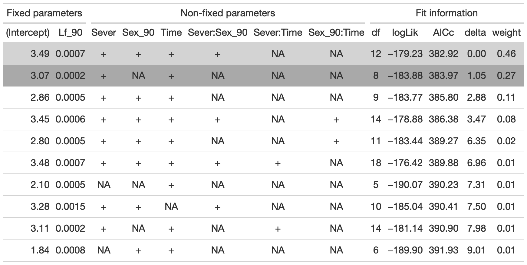
From this round of model selection, when lf_90 is required to be in the models that are considered, there are two models with equivalently low AICc values: one has sever, sex_90, time, lf_90, and the sever x sex_90 interaction (AICc: 382.9). The other model has only Sever, Time, and Lf_90 (AICc: 384).
3.1.3 Model selection without leaf area
## Fixed terms are "cond((Int))" and "disp((Int))"tab <- head(dr, n=10) %>% gt() %>% cols_hide(columns=vars(`disp((Int))`)) %>%
cols_label(`cond((Int))`="(Intercept)", `cond(Lf_90)`="Lf_90", `cond(Sever)`="Sever", `cond(Sex_90)`="Sex_90", `cond(Time)`="Time", `cond(Sever:Sex_90)`="Sever:Sex_90", `cond(Sever:Time)`="Sever:Time", `cond(Sex_90:Time)`= "Sex_90:Time") %>%
fmt_number(columns = vars(`cond((Int))`, logLik, AICc, delta, weight), decimals = 2) %>%
fmt_number(columns = vars(`cond(Lf_90)`), decimals = 4) %>%
tab_spanner(label = "Fit information", columns = vars(df, logLik, AICc, delta, weight)) %>%
tab_spanner(label = "Non-fixed parameters", columns = vars(`cond((Int))`, `cond(Lf_90)`, `cond(Sever)`, `cond(Sex_90)`, `cond(Time)`, `cond(Sever:Sex_90)`, `cond(Sever:Time)`, `cond(Sex_90:Time)`)) %>%
tab_spanner(label = "Fixed parameters", columns = vars(`cond((Int))`)) %>%
tab_style(style = cell_fill(color = "lightgrey"), locations = cells_body(columns = everything(),rows = delta <= 2)) %>%
tab_style(style = cell_fill(color = "darkgrey"), locations = cells_body( columns = everything(), rows = 2))
tab %>% gtsave("front_91_sur_b.png", vwidth=1200) 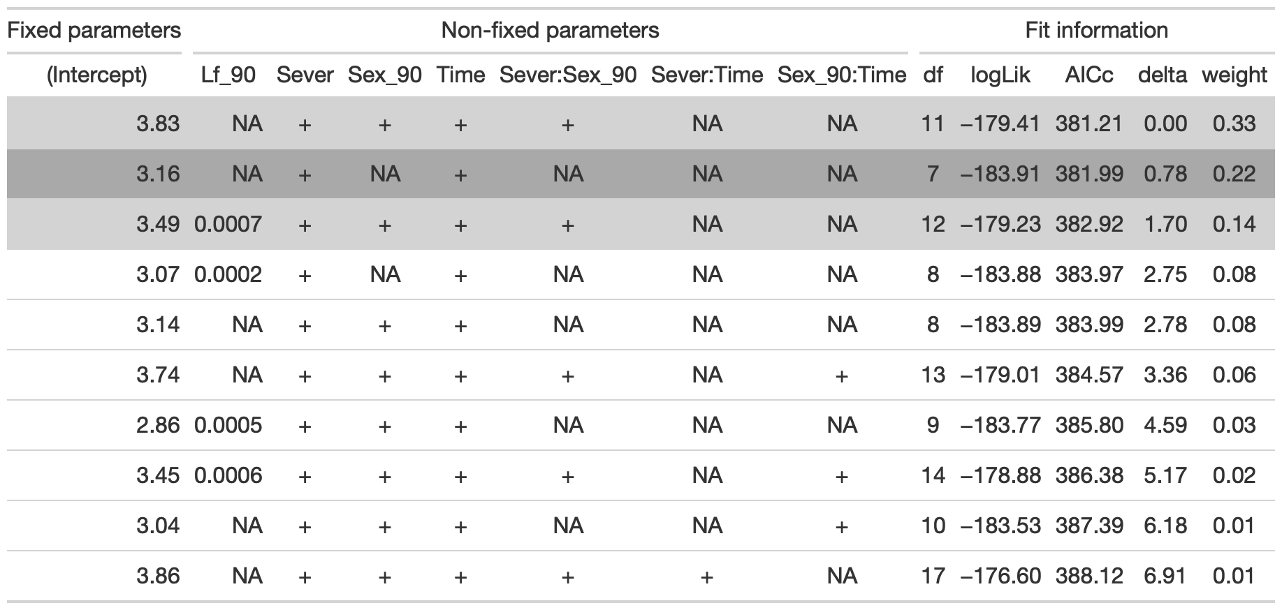
From this round of model selection, when lf_90 is not required to be in the models that are considered, there are three models with equivalently low AICc values: one has Sever, Sex_90, Time, and the sever x sex_90 interaction (AICc: 381.2). The second has Sever and Time (AICc: 382). The third has sever, sex_90, time, lf_90, and the sever x sex_90 interaction (AICc: 382.9)–this was also one of the top two models when leaf area in 1990 was fixed.
3.1.4 Conclusion
sur_91f_bm<-glmmTMB(deadAliveBinary~ Sever+Time +  (1|COLONY), data = mayappleData,
                family="binomial")
The best model for survival of the front shoot in 1991 contains fixed effects of Sever and Time.
3.1.5 Estimated marginal means
The main effect of severing
g1<- ggplot(data=mayappleData, aes(x=Sever, y=deadAliveBinary)) +
  geom_bar(stat="summary", fun.y = "mean", position = "dodge") +
  ylab("Mean of binary response for\n dead/alive")

emmeans(sur_91f_bm, pairwise~Sever, type="response" )
## $emmeans
## Sever prob SE df lower.CL upper.CL
## C 0.975 0.0115 673 0.939 0.990
## S1 0.897 0.0289 673 0.825 0.942
## S2 0.947 0.0187 673 0.895 0.973
## S4 0.947 0.0187 673 0.896 0.974
##
## Results are averaged over the levels of: Time
## Confidence level used: 0.95
## Intervals are back-transformed from the logit scale
##
## $contrasts
## contrast odds.ratio SE df t.ratio p.value
## C / S1 4.390 2.021 673 3.213 0.0075
## C / S2 2.160 1.062 673 1.565 0.3992
## C / S4 2.130 1.048 673 1.537 0.4157
## S1 / S2 0.492 0.184 673 -1.901 0.2284
## S1 / S4 0.485 0.181 673 -1.935 0.2143
## S2 / S4 0.986 0.407 673 -0.033 1.0000
##
## Results are averaged over the levels of: Time
## P value adjustment: tukey method for comparing a family of 4 estimates
## Tests are performed on the log odds ratio scale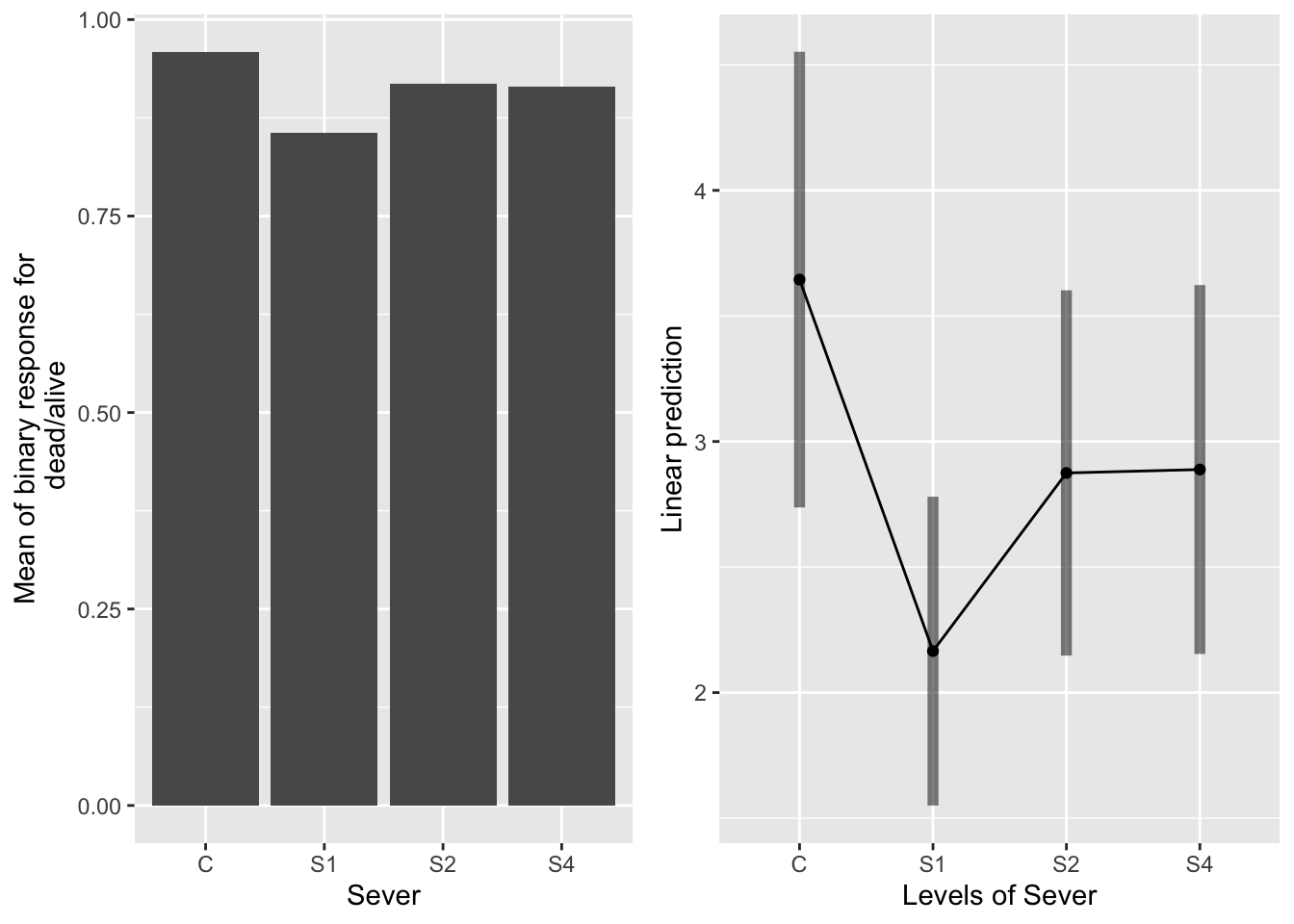
S1 has a lower probability of survival than control systems.
The main effect of time
g1<-ggplot(data=mayappleData, aes(x=Time, y=deadAliveBinary)) +
  geom_bar(stat="summary", fun.y = "mean", position = "dodge") +
  ylab("Mean of binary response for\n dead/alive")

emmeans(sur_91f_bm, pairwise~Time, type="response" )
## $emmeans
## Time prob SE df lower.CL upper.CL
## T1 0.918 0.02305 673 0.860 0.953
## T2 0.925 0.02157 673 0.870 0.958
## T3 0.977 0.00983 673 0.947 0.990
##
## Results are averaged over the levels of: Sever
## Confidence level used: 0.95
## Intervals are back-transformed from the logit scale
##
## $contrasts
## contrast odds.ratio SE df t.ratio p.value
## T1 / T2 0.907 0.283 673 -0.313 0.9475
## T1 / T3 0.261 0.112 673 -3.119 0.0054
## T2 / T3 0.288 0.125 673 -2.873 0.0117
##
## Results are averaged over the levels of: Sever
## P value adjustment: tukey method for comparing a family of 3 estimates
## Tests are performed on the log odds ratio scale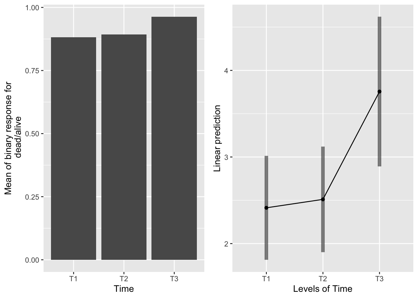
Again, the CIs all overlap, but the contrasts between T1-T3 and T2-T3 are significant, indicating higher survival in the T3 systems. Also, with looking at time in isolation from the other factors, we have to keep in mind that the control systems are part of each time, so actual severing did not occur for each system at all times.
3.2 Leaf area
This analysis is the conditional leaf area–excludes the zero systems.
3.2.1 Conditional data & visualization
mayappleData$LfFtot_91<-as.numeric(mayappleData$LfFtot_91)

mayappleData <- mayappleData %>%
  filter(!is.na(LfFtot_91)) %>%
  filter(LfFtot_91>0)

ggplot(data=mayappleData, aes(x=Sever, y=LfFtot_91, fill = Time)) +
   stat_summary(fun = mean, geom = "bar",position="dodge") +
    stat_summary(fun.data = mean_se, geom = "errorbar", position="dodge")+
  facet_wrap(~Sex_90) +
  ylab("Mean of total leaf area \n for branches in front of plant") +
  scale_fill_brewer(palette="Set1")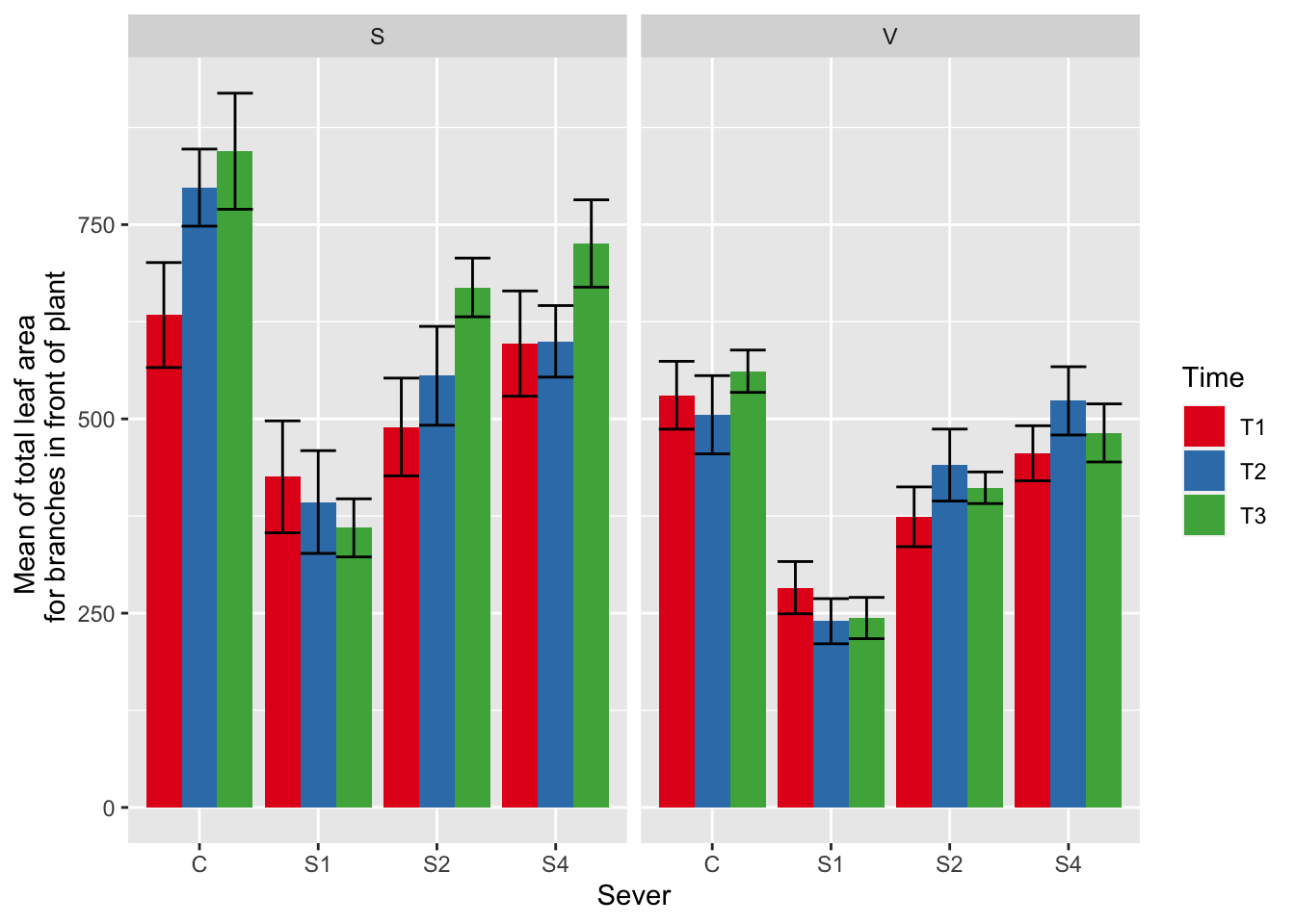
3.2.2 Conditional Model selection
mod91laf<-lmer(LfFtot_91~Sex_90*Sever*Time+Lf_90 +(1|COLONY), data = mayappleData, na.action ="na.fail", REML=FALSE)
dr<-dredge(mod91laf)
tab <- head(dr, n=10) %>% gt() %>%
  fmt_number(columns = vars(`(Intercept)`, Lf_90,  logLik, AICc, delta, weight), decimals = 2) %>%
  tab_spanner(label = "Fit information", columns = vars(df, logLik, AICc, delta, weight)) %>%
  tab_spanner(label = "Non-fixed parameters", columns = vars(`(Intercept)`,   Lf_90,  Sever, Sex_90, Time,  `Sever:Sex_90`, `Sever:Time`, `Sex_90:Time`, `Sever:Sex_90:Time`)) %>%
  tab_spanner(label = "Fixed parameters", columns = vars(`(Intercept)`)) %>%
    tab_style(style = cell_fill(color = "lightgrey"), locations = cells_body(columns = everything(),rows = delta <= 2)) %>%
  tab_style(style = cell_fill(color = "darkgrey"), locations = cells_body( columns = everything(), rows = 4))


tab %>% gtsave("front_91_leaf_conditional.png", vwidth=1200) 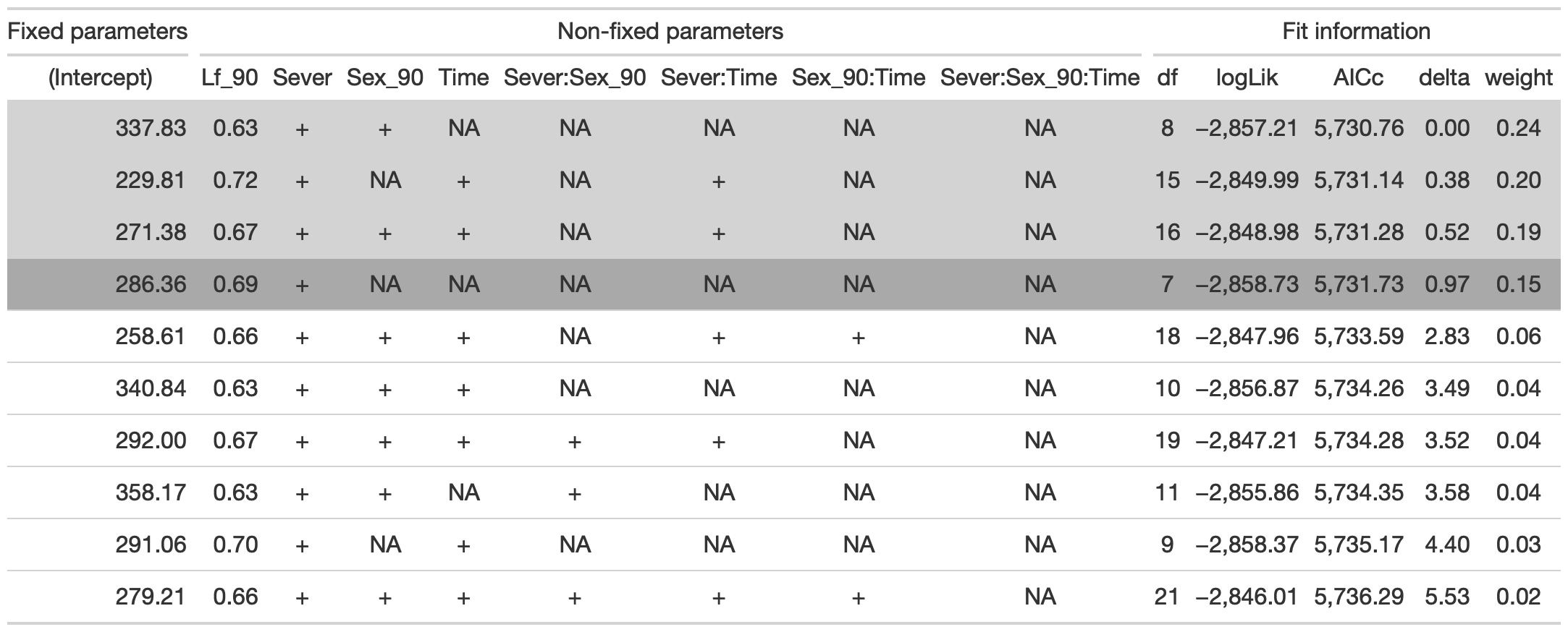
From this round of model selection, when Lf_90 is not required to be in the models that are considered, the simplest model contains Lf_90 and Sever.
3.2.3 Conclusion
The simplest and best model contains fixed effects of Lf_90 and Sever.
3.2.4 Estimated marginal means
the main effect of sever
g1 <- ggplot(data=mayappleData, aes(x=Sever, y=LfFtot_91)) +
  geom_bar(stat="summary", fun.y = "mean", position = "dodge") +
  ylab("Mean of total leaf area \n for branches in front of plant")

emmeans(mod91laf.bm, pairwise~Sever, type="response")
## $emmeans
## Sever emmean SE df lower.CL upper.CL
## C 633 18.0 156 598 669
## S1 326 21.6 222 284 369
## S2 491 19.1 186 453 528
## S4 556 18.5 166 519 592
##
## Degrees-of-freedom method: satterthwaite
## Confidence level used: 0.95
##
## $contrasts
## contrast estimate SE df t.ratio p.value
## C - S1 307.1 26.2 415 11.716 <.0001
## C - S2 142.7 24.3 412 5.862 <.0001
## C - S4 77.5 23.8 412 3.253 0.0067
## S1 - S2 -164.4 27.1 419 -6.072 <.0001
## S1 - S4 -229.5 26.7 423 -8.599 <.0001
## S2 - S4 -65.2 24.7 413 -2.633 0.0434
##
## Degrees-of-freedom method: satterthwaite
## P value adjustment: tukey method for comparing a family of 4 estimates
Control systems have the most leaf area, then S4, then S2, then S1. All contrasts are significant.
the main effect of leaf area
ggplot(data=mayappleData, aes(x=Lf_90, y=LfFtot_91, color=Sever)) +
  geom_point() + geom_smooth(method = "glm", se = FALSE, formula=y~poly(x,2))+
  facet_wrap(~Time) +
ylab("Mean of total leaf area \n for branches in front of plant") 
This analysis uses data from all systems (e.g. dead systems would have a leaf area of 0 and be included) so it is the product of survival and growth.
3.2.5 Product Data & visualization
mayappleData$LfFtot_91<-as.numeric(mayappleData$LfFtot_91)

mayappleData <- mayappleData %>%
  filter(!is.na(LfFtot_91))

ggplot(data=mayappleData, aes(x=Sever, y=LfFtot_91, fill = Time)) +
   stat_summary(fun = mean, geom = "bar",position="dodge") +
    stat_summary(fun.data = mean_se, geom = "errorbar", position="dodge")+
  facet_wrap(~Sex_90) +
  ylab("Mean of total leaf area \n for branches in front of plant") +
  scale_fill_brewer(palette="Set1")
3.2.6 Model selection with leaf area
mod91laf<-lmer(LfFtot_91~Sex_90*Sever*Time+Lf_90 +(1|COLONY), data = mayappleData, na.action ="na.fail", REML=FALSE)
#this is the global model
#MuMIn::getAllTerms(mod91laf) #this lets us see how to specify terms in the model

dr<-dredge(mod91laf, fixed=~Lf_90)

tab <- head(dr, n=10) %>% gt() %>%
  fmt_number(columns = vars(`(Intercept)`, Lf_90,  logLik, AICc, delta, weight), decimals = 2) %>%
  tab_spanner(label = "Fit information", columns = vars(df, logLik, AICc, delta, weight)) %>%
  tab_spanner(label = "Non-fixed parameters", columns = vars(`(Intercept)`,   Lf_90,  Sever, Sex_90, Time,  `Sever:Sex_90`, `Sever:Time`, `Sex_90:Time`, `Sever:Sex_90:Time`)) %>%
  tab_spanner(label = "Fixed parameters", columns = vars(`(Intercept)`,Lf_90)) %>%
    tab_style(style = cell_fill(color = "lightgrey"), locations = cells_body(columns = everything(),rows = delta <= 2)) %>%
  tab_style(style = cell_fill(color = "darkgrey"), locations = cells_body( columns = everything(), rows = 1))


tab %>% gtsave("front_91_leaf_a.png", vwidth=1200) 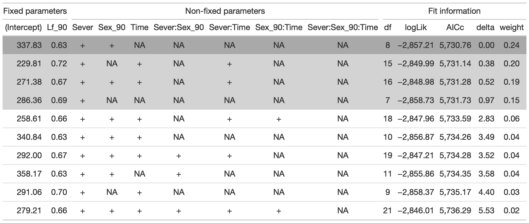
From this round of model selection, when Lf_90 is required to be in the models that are considered, there are four models within two AICc units: (1) Lf_90, Sever, Sex_90, Time, and the Sever x Sex_90 interaction (AICc: 6738.5); (2) Lf_90, Sever, Sex_90, Time, the Sever x Sex_90 interaction, and the Sex_90 x Time interaction (AICc 6738.8); (3) Lf_90, Sever, Sex_90, Time, the Sever x Sex_90 interaction, and the Sever x Time interaction (AICc 6740.1); (4) Lf_90, Sever, Sex_90, Time, and all three two-way interactions (AICc 6740.2)
3.2.7 Model selection without leaf area
dr<-dredge(mod91laf)
tab <- head(dr, n=10) %>% gt() %>%
  fmt_number(columns = vars(`(Intercept)`, Lf_90,  logLik, AICc, delta, weight), decimals = 2) %>%
  tab_spanner(label = "Fit information", columns = vars(df, logLik, AICc, delta, weight)) %>%
  tab_spanner(label = "Non-fixed parameters", columns = vars(`(Intercept)`,   Lf_90,  Sever, Sex_90, Time,  `Sever:Sex_90`, `Sever:Time`, `Sex_90:Time`, `Sever:Sex_90:Time`)) %>%
  tab_spanner(label = "Fixed parameters", columns = vars(`(Intercept)`)) %>%
    tab_style(style = cell_fill(color = "lightgrey"), locations = cells_body(columns = everything(),rows = delta <= 2)) %>%
  tab_style(style = cell_fill(color = "darkgrey"), locations = cells_body( columns = everything(), rows = 1))


tab %>% gtsave("front_91_leaf_b.png", vwidth=1200) 
From this round of model selection, when Lf_90 is not required to be in the models that are considered, the same four models as above are returned.
3.2.8 Conclusion
The simplest and best model contains fixed effects of Lf_90, Sever, Sex_90, Time, and the Sever x Sex_90 interaction.
3.2.9 Estimated marginal means
the sex x sever interaction
g1 <- ggplot(data=mayappleData, aes(x=Sever, y=LfFtot_91, fill=Sex_90)) +
  geom_bar(stat="summary", fun.y = "mean", position = "dodge") +
  ylab("Mean of total leaf area \n for branches in front of plant")

emmeans(mod91laf.bm, pairwise~Sex_90|Sever, type="response")
## $emmeans
## Sever = C:
## Sex_90 emmean SE df lower.CL upper.CL
## S 676 26.0 343 625 727
## V 597 24.4 317 549 645
##
## Sever = S1:
## Sex_90 emmean SE df lower.CL upper.CL
## S 325 29.9 359 266 384
## V 327 30.7 375 267 388
##
## Sever = S2:
## Sex_90 emmean SE df lower.CL upper.CL
## S 511 27.2 356 458 565
## V 471 26.2 339 420 523
##
## Sever = S4:
## Sex_90 emmean SE df lower.CL upper.CL
## S 568 26.7 344 516 621
## V 545 25.1 324 496 595
##
## Results are averaged over the levels of: Time
## Degrees-of-freedom method: satterthwaite
## Confidence level used: 0.95
##
## $contrasts
## Sever = C:
## contrast estimate SE df t.ratio p.value
## S - V 79.17 35.8 415 2.214 0.0273
##
## Sever = S1:
## contrast estimate SE df t.ratio p.value
## S - V -2.01 42.8 424 -0.047 0.9625
##
## Sever = S2:
## contrast estimate SE df t.ratio p.value
## S - V 39.76 37.5 420 1.059 0.2903
##
## Sever = S4:
## contrast estimate SE df t.ratio p.value
## S - V 23.08 36.6 418 0.631 0.5281
##
## Results are averaged over the levels of: Time
## Degrees-of-freedom method: satterthwaite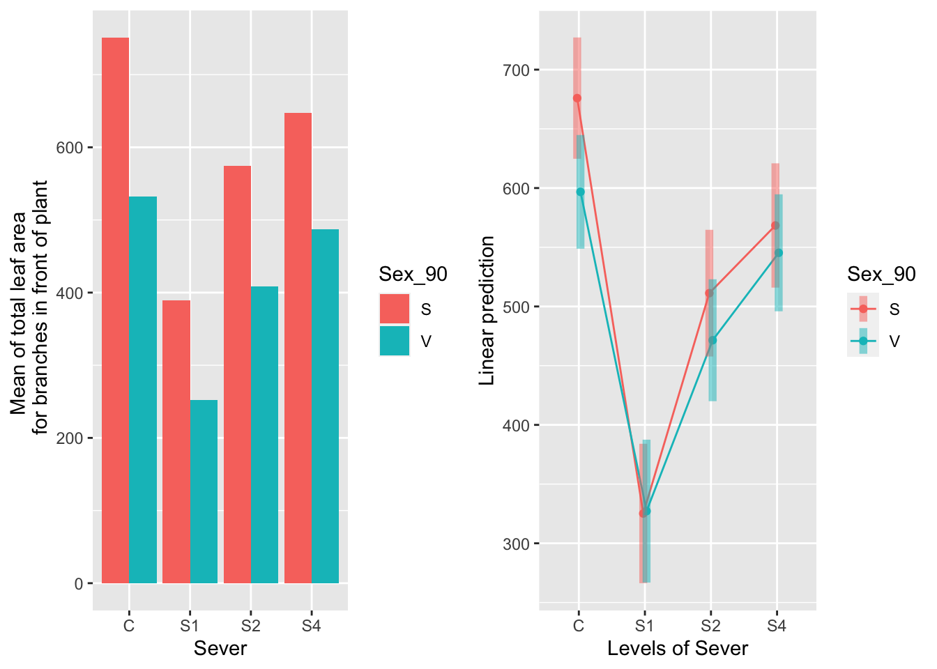
Sexual systems have more leaf area in the control treatment. In all other severing treatments, sexual and vegetative systems have approximately the same amount of leaf area.
the main effect of sex
g1 <- ggplot(data=mayappleData, aes(x=Sex_90, y=LfFtot_91)) +
  geom_bar(stat="summary", fun.y = "mean", position = "dodge") +
  ylab("Mean of total leaf area \n for branches in front of plant")

emmeans(mod91laf.bm, pairwise~Sex_90, type="response")
## $emmeans
## Sex_90 emmean SE df lower.CL upper.CL
## S 520 16.1 106.1 488 552
## V 485 15.7 99.1 454 516
##
## Results are averaged over the levels of: Sever, Time
## Degrees-of-freedom method: satterthwaite
## Confidence level used: 0.95
##
## $contrasts
## contrast estimate SE df t.ratio p.value
## S - V 35 22.4 429 1.561 0.1192
##
## Results are averaged over the levels of: Sever, Time
## Degrees-of-freedom method: satterthwaite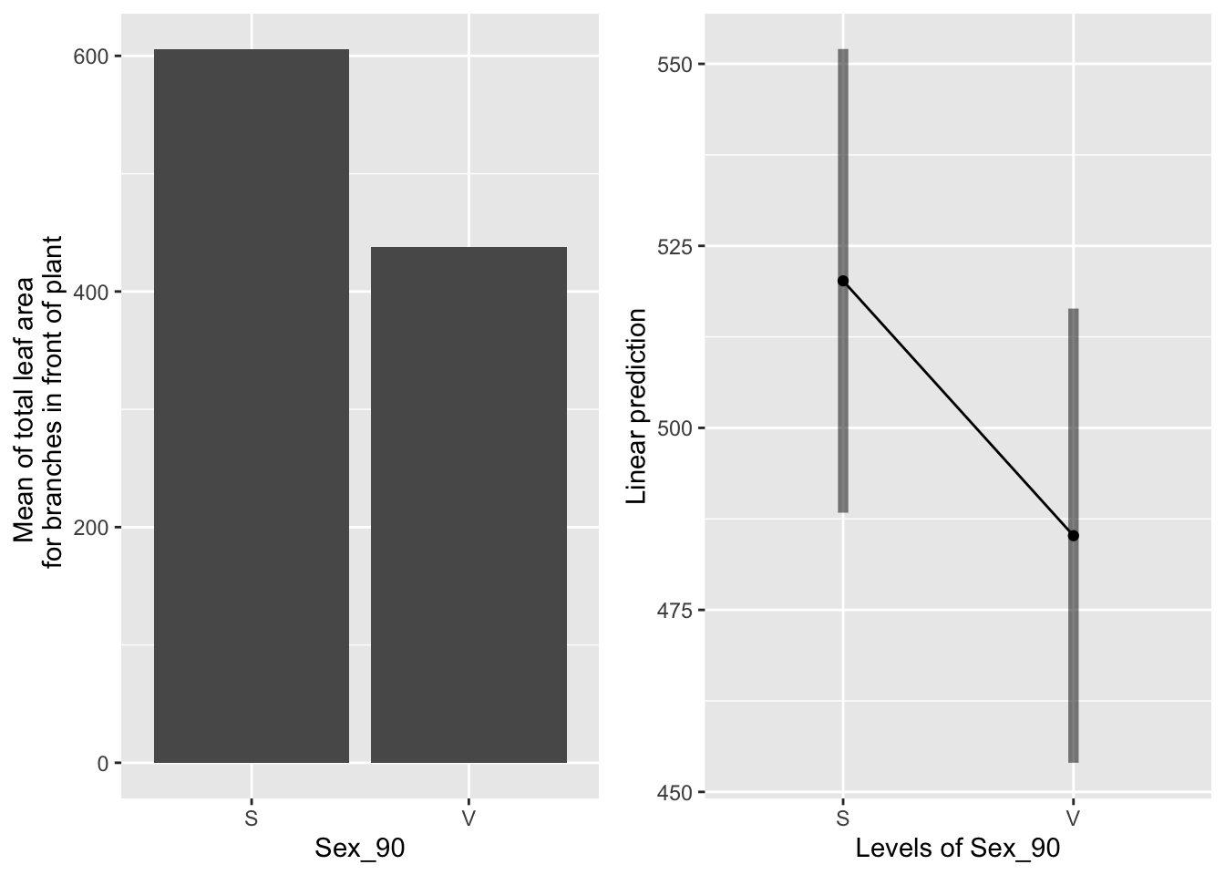
Sexual systems have more leaf area overall, but this is not significant.
the main effect of sever
g1 <- ggplot(data=mayappleData, aes(x=Sever, y=LfFtot_91)) +
  geom_bar(stat="summary", fun.y = "mean", position = "dodge") +
  ylab("Mean of total leaf area \n for branches in front of plant")

emmeans(mod91laf.bm, pairwise~Sever, type="response")
## $emmeans
## Sever emmean SE df lower.CL upper.CL
## C 636 17.8 161 601 672
## S1 326 21.5 227 284 368
## S2 491 19.0 191 454 529
## S4 557 18.4 171 521 593
##
## Results are averaged over the levels of: Sex_90, Time
## Degrees-of-freedom method: satterthwaite
## Confidence level used: 0.95
##
## $contrasts
## contrast estimate SE df t.ratio p.value
## C - S1 310.2 26.1 416 11.872 <.0001
## C - S2 145.0 24.2 413 5.987 <.0001
## C - S4 79.5 23.7 413 3.352 0.0048
## S1 - S2 -165.2 26.9 420 -6.135 <.0001
## S1 - S4 -230.7 26.6 424 -8.680 <.0001
## S2 - S4 -65.5 24.6 414 -2.661 0.0402
##
## Results are averaged over the levels of: Sex_90, Time
## Degrees-of-freedom method: satterthwaite
## P value adjustment: tukey method for comparing a family of 4 estimates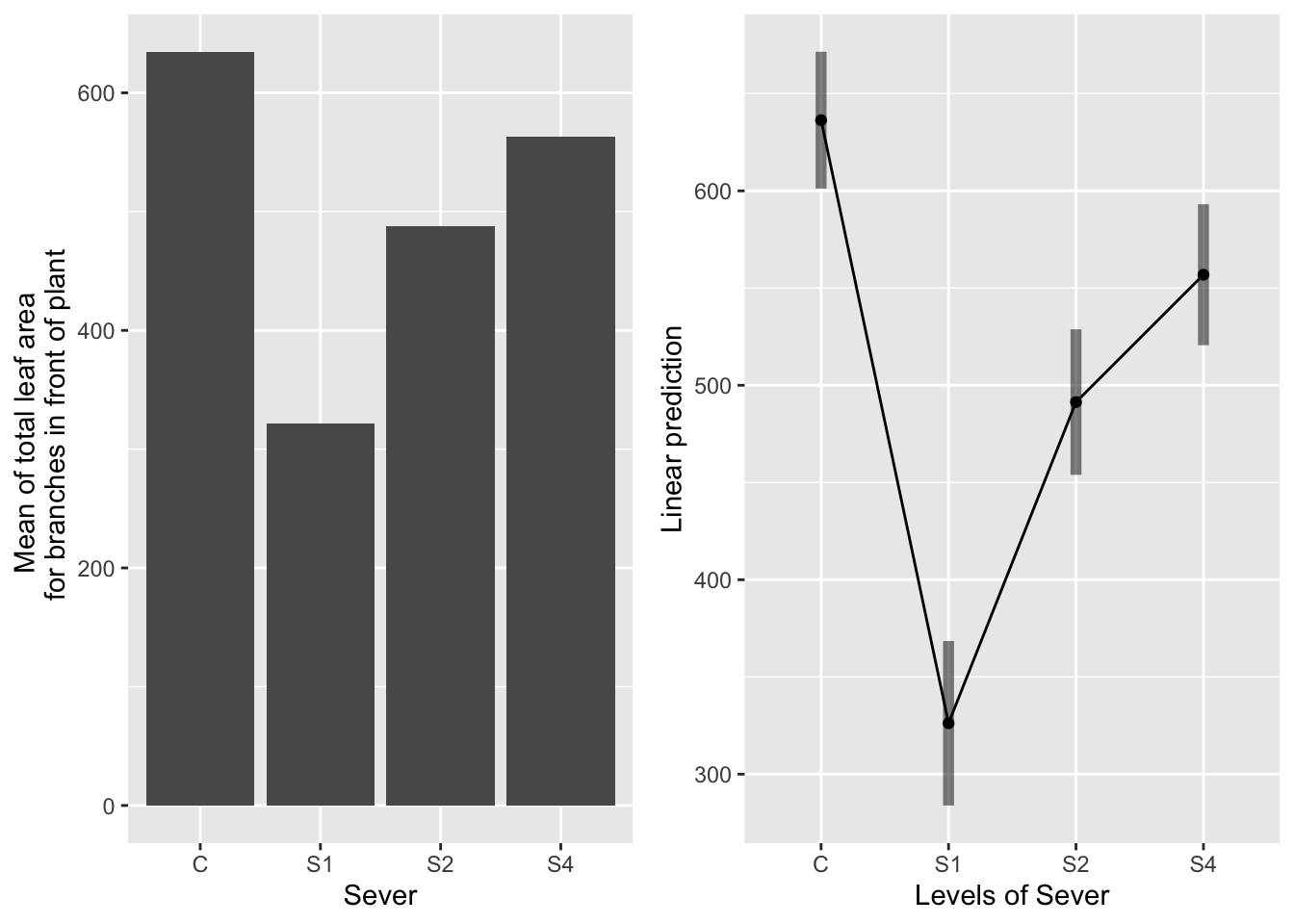
Control systems have the most leaf area. S1 systems have the least leaf area. S2 and S4 systems are intermediate and not different from each other.
the main effect of time
g1 <-ggplot(data=mayappleData, aes(x=Time, y=LfFtot_91)) +
  geom_bar(stat="summary", fun.y = "mean", position = "dodge") +
  ylab("Mean of total leaf area \n for branches in front of plant")

emmeans(mod91laf.bm, pairwise~Time, type="response")
## $emmeans
## Time emmean SE df lower.CL upper.CL
## T1 504 18.1 156 468 540
## T2 493 16.4 122 461 526
## T3 511 16.8 128 478 544
##
## Results are averaged over the levels of: Sex_90, Sever
## Degrees-of-freedom method: satterthwaite
## Confidence level used: 0.95
##
## $contrasts
## contrast estimate SE df t.ratio p.value
## T1 - T2 10.89 22.6 417 0.482 0.8797
## T1 - T3 -6.88 23.2 421 -0.297 0.9525
## T2 - T3 -17.77 21.3 421 -0.836 0.6811
##
## Results are averaged over the levels of: Sex_90, Sever
## Degrees-of-freedom method: satterthwaite
## P value adjustment: tukey method for comparing a family of 3 estimates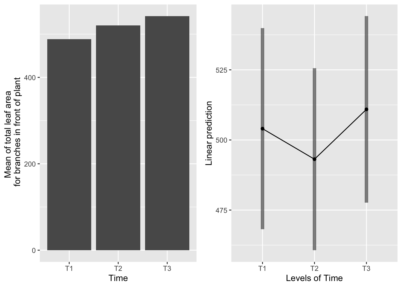
T1 and T2 have the same amount of leaf area. T3 has significantly more leaf area than T2, but not T1.
the main effect of leaf area
ggplot(data=mayappleData, aes(x=Lf_90, y=LfFtot_91, color=Sever)) +
  geom_point() + geom_smooth(method = "glm", se = FALSE, formula=y~poly(x,2))+
  facet_wrap(~Time) +
ylab("Mean of total leaf area \n for branches in front of plant") 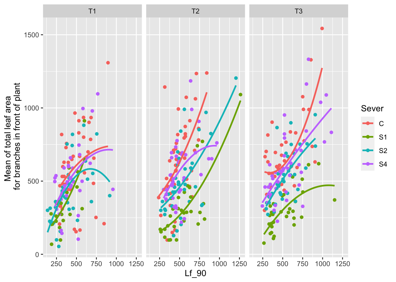
plots for MS
g1 <- emmip(mod91laf.bm,  Sex_90 ~ Sever  ,CIs = TRUE)+ ggtitle("The sex x sever interaction") +
  theme_bw()+theme(plot.title = element_text(face="italic"))+theme(panel.grid.major = element_blank(), panel.grid.minor = element_blank())
## Cannot use mode = "kenward-roger" because *pbkrtest* package is not installedg2 <- emmip(mod91laf.bm, ~ Sex_90 ,CIs = TRUE) +ggtitle("The main effect of sex")+
theme_bw()+theme(plot.title = element_text(face="italic"))+theme(panel.grid.major = element_blank(), panel.grid.minor = element_blank())## Cannot use mode = "kenward-roger" because *pbkrtest* package is not installed## NOTE: Results may be misleading due to involvement in interactionsg3 <- emmip(mod91laf.bm, ~ Sever ,CIs = TRUE) +ggtitle("The main effect of sever")+
theme_bw()+theme(plot.title = element_text(face="italic"))+theme(panel.grid.major = element_blank(), panel.grid.minor = element_blank())## Cannot use mode = "kenward-roger" because *pbkrtest* package is not installed
## NOTE: Results may be misleading due to involvement in interactionsg4 <- emmip(mod91laf.bm, ~ Time ,CIs = TRUE) + ggtitle("The main effect of time") +
theme_bw()+theme(plot.title = element_text(face="italic"))+theme(panel.grid.major = element_blank(), panel.grid.minor = element_blank())## Cannot use mode = "kenward-roger" because *pbkrtest* package is not installedmylist <- list(Lf_90=seq(150,1250,by=100))
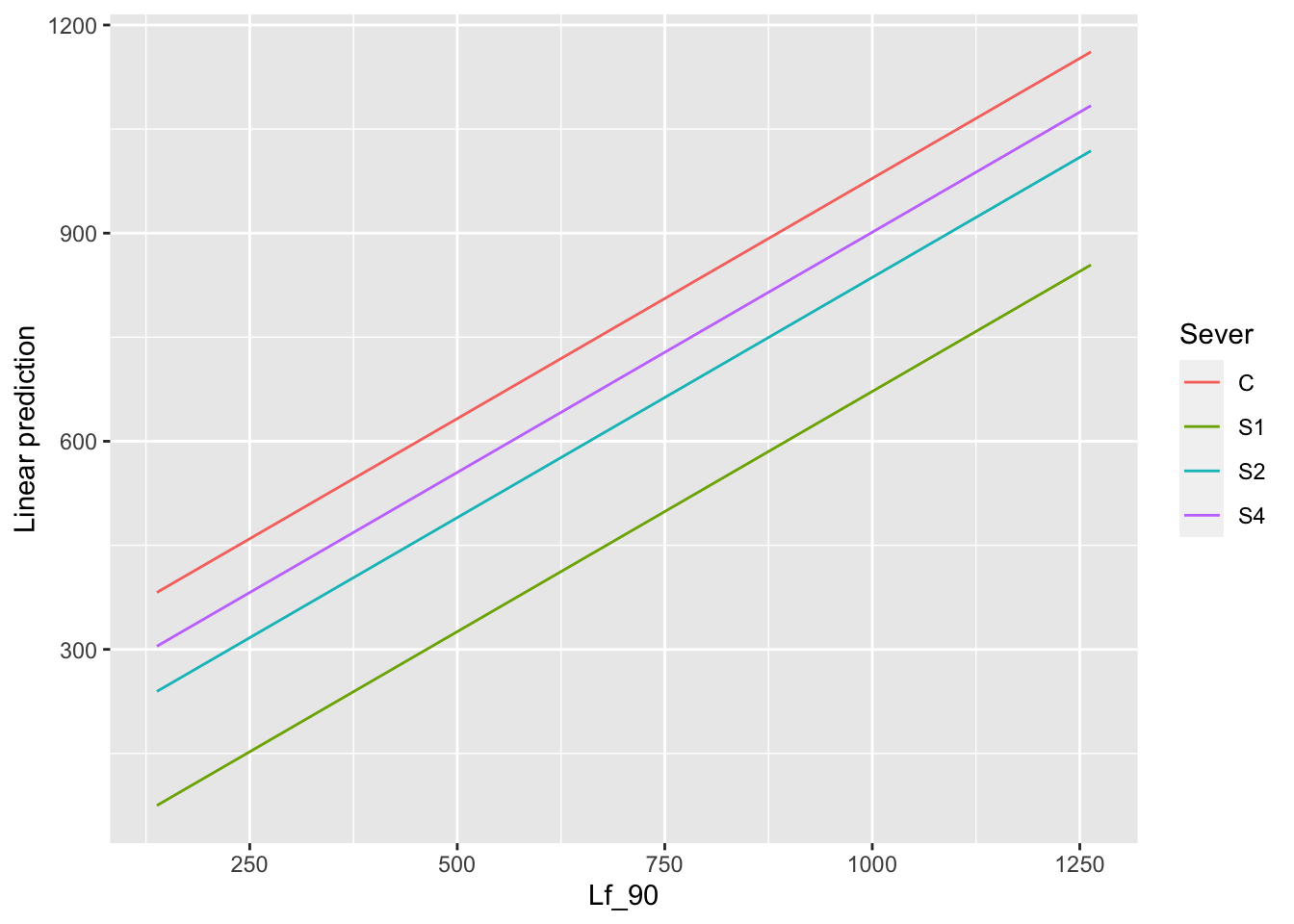
g5 <- emmip(mod91laf.bm, ~ Lf_90 , at=mylist, CIs = TRUE) + ggtitle("The main effect of Lf_1990") +
theme_bw()+theme(plot.title = element_text(face="italic"))+theme(panel.grid.major = element_blank(), panel.grid.minor = element_blank())## Cannot use mode = "kenward-roger" because *pbkrtest* package is not installedlibrary("cowplot")
ggdraw()+
draw_plot(g1, x=0, y=0.33, width = .5, height = .67)+
draw_plot(g2, x=0.5, y=0.67, width = 0.5, height = 0.33 ) +
draw_plot(g3, x=0.5, y=0.33, width = 0.5, height = 0.33) +
draw_plot(g4, x=0, y=0, width = 0.5, height = 0.33) +
draw_plot(g5, x=0.5, y=0,width = 0.5, height = 0.33 )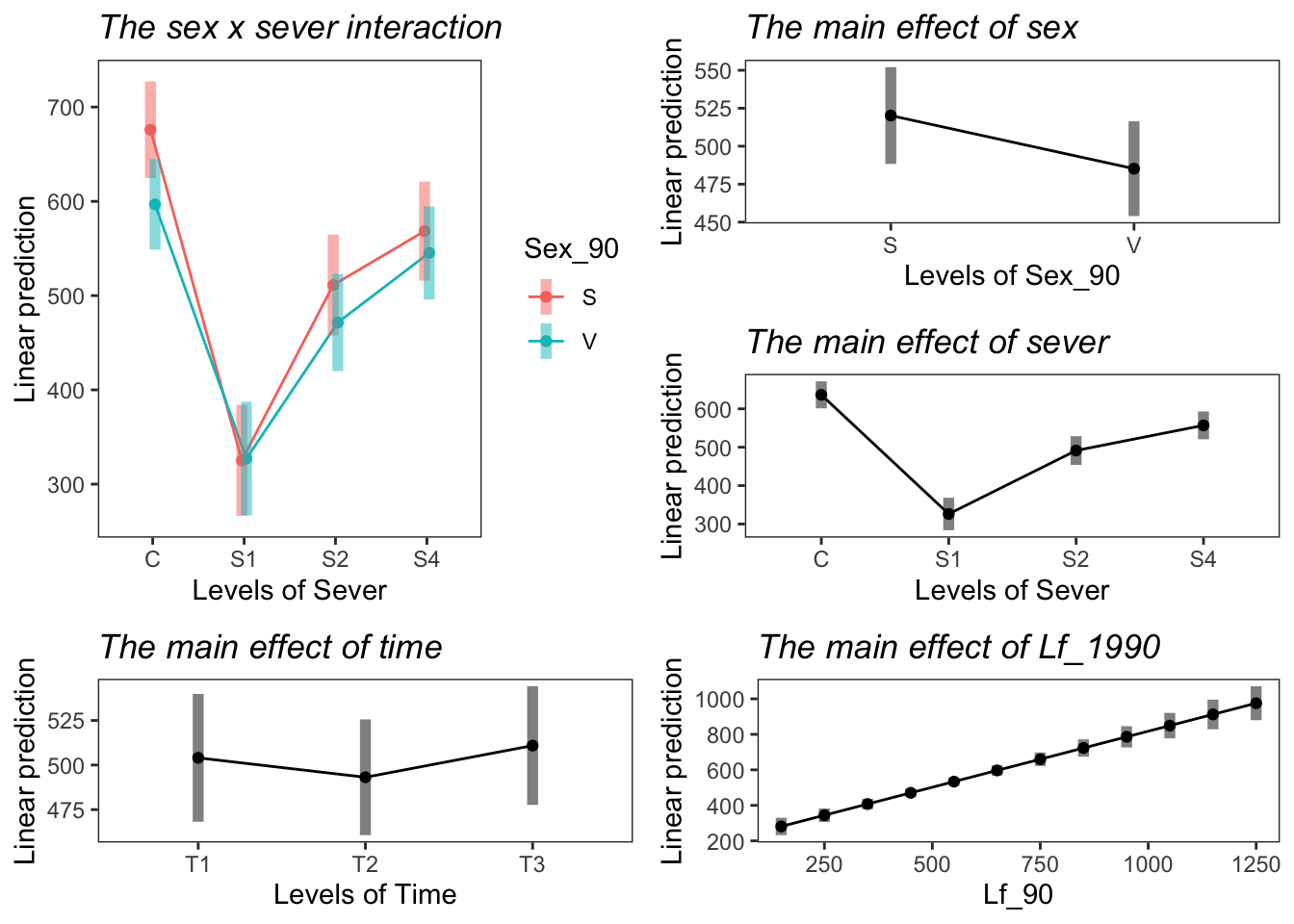
3.3 Branching
For these analyses, we filtered the dataset to only plants that are alive (1 or more branches) and created a binary variable for whether plants have 1 branch, or more than 1 branch.
3.3.1 Data & visualization
# filter the dataset to only plants that are alive (1 or more branches)
# create binary variable for plants that are have 1 branch (0) or more than 1 branch (1)
# append new variable to the new (filtered) dataframe
mayappleDatasetFull<-readxl::read_excel("Datasets/mayapple_1990_updated.xlsx", na=".")

mayappleData <- mayappleDatasetFull %>%
  dplyr::select(COLONY,Lf_90,brnoF_91,Sex_90,Sever,Time,SexF1_91,SexF2_91,SexF3_91,LfFtot_91) %>%
  filter(!is.na(Lf_90))


mayappleAliveData <- mayappleData %>%
  filter(!is.na(Lf_90)) %>%
  dplyr::filter(brnoF_91>=1) %>%
  dplyr::mutate(branchingBinary=ifelse(brnoF_91>1,1,0))

# create a plot showing the mean of the binary response variable in each category
# interpretation for values = 0, all responses were 0 in that category (all plants have 1 branch)
# interpretation for values = 1, all responses were 1 in that category (all plants have >1 branch)
ggplot(data=mayappleAliveData, aes(x=Sever, y=branchingBinary, fill = Time)) +
  stat_summary(fun = mean, geom = "bar",position="dodge") +
  stat_summary(fun.data = mean_se, geom = "errorbar", position="dodge")+
  facet_wrap(~Sex_90) +
  ylab("Mean of binary response for\n not branching/branching ") +
  scale_fill_brewer(palette="Set1")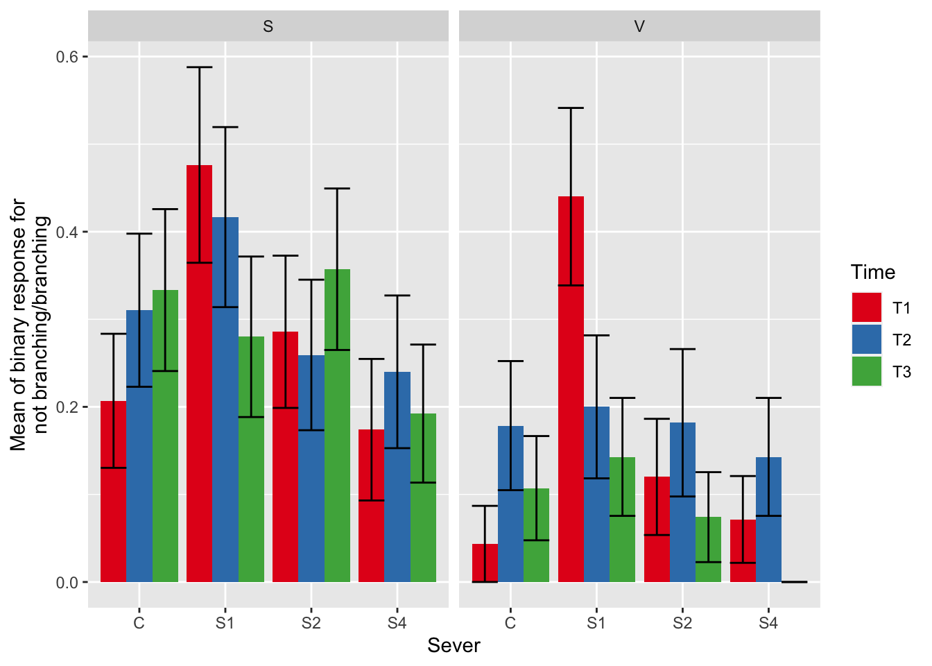
3.3.2 Model selection with leaf area
mod91brl<-glmmTMB(branchingBinary~ Sex_90*Sever*Time +  Lf_90 + (1|COLONY), data = mayappleAliveData,
                family="binomial")

#this is the global model
#MuMIn::getAllTerms(mod91brl) #this lets us see how to specify terms in the model

dr<-dredge(mod91brl, fixed=~cond(Lf_90))

tab <- head(dr, n=10) %>% gt() %>% cols_hide(columns=vars(`disp((Int))`)) %>%
  cols_label(`cond((Int))`="(Intercept)", `cond(Lf_90)`="Lf_90", `cond(Sever)`="Sever", `cond(Sex_90)`="Sex_90", `cond(Time)`="Time", `cond(Sever:Sex_90)`="Sever:Sex_90", `cond(Sever:Time)`="Sever:Time", `cond(Sex_90:Time)`= "Sex_90:Time") %>%
  fmt_number(columns = vars(`cond((Int))`, logLik, AICc, delta, weight), decimals = 2) %>%
  fmt_number(columns = vars(`cond(Lf_90)`), decimals = 4) %>%
  tab_spanner(label = "Fit information", columns = vars(df, logLik, AICc, delta, weight)) %>%
  tab_spanner(label = "Non-fixed parameters", columns = vars(`cond((Int))`,  `cond(Lf_90)`, `cond(Sever)`, `cond(Sex_90)`, `cond(Time)`, `cond(Sever:Sex_90)`, `cond(Sever:Time)`, `cond(Sex_90:Time)`)) %>%
  tab_spanner(label = "Fixed parameters", columns = vars(`cond((Int))`,  `cond(Lf_90)`)) %>%
    tab_style(style = cell_fill(color = "lightgrey"), locations = cells_body(columns = everything(),rows = delta <= 2)) %>%
  tab_style(style = cell_fill(color = "darkgrey"), locations = cells_body( columns = everything(), rows = 1))


tab %>% gtsave("front_91_br_a.png", vwidth=1200) 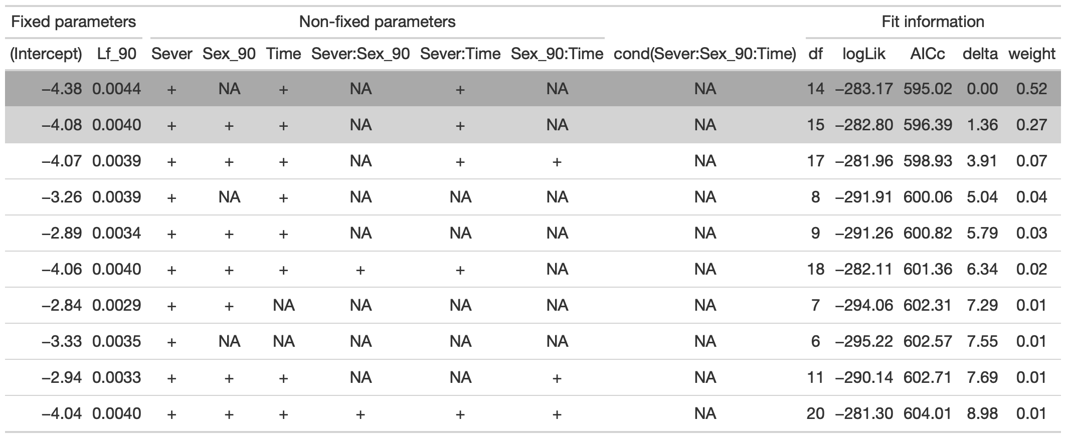
From this round of model selection, when Lf_90 is required to be in the models that are considered, there are two models within 2 AICc units: (1) Lf_90, Sever, Time, and Sever x Time (AICc 595); (2) Lf_90, Sever, Sex, Time, and Sever x Time (AICc 596.4).
3.3.3 Model selection without leaf area
dr<-dredge(mod91brl)

tab <- head(dr, n=10) %>% gt() %>% cols_hide(columns=vars(`disp((Int))`)) %>%
  cols_label(`cond((Int))`="(Intercept)", `cond(Lf_90)`="Lf_90", `cond(Sever)`="Sever", `cond(Sex_90)`="Sex_90", `cond(Time)`="Time", `cond(Sever:Sex_90)`="Sever:Sex_90", `cond(Sever:Time)`="Sever:Time", `cond(Sex_90:Time)`= "Sex_90:Time") %>%
  fmt_number(columns = vars(`cond((Int))`, logLik, AICc, delta, weight), decimals = 2) %>%
  fmt_number(columns = vars(`cond(Lf_90)`), decimals = 4) %>%
  tab_spanner(label = "Fit information", columns = vars(df, logLik, AICc, delta, weight)) %>%
  tab_spanner(label = "Non-fixed parameters", columns = vars(`cond((Int))`,  `cond(Lf_90)`, `cond(Sever)`, `cond(Sex_90)`, `cond(Time)`, `cond(Sever:Sex_90)`, `cond(Sever:Time)`, `cond(Sex_90:Time)`)) %>%
  tab_spanner(label = "Fixed parameters", columns = vars(`cond((Int))`)) %>%
    tab_style(style = cell_fill(color = "lightgrey"), locations = cells_body(columns = everything(),rows = delta <= 2)) %>%
  tab_style(style = cell_fill(color = "darkgrey"), locations = cells_body( columns = everything(), rows = 1))


tab %>% gtsave("front_91_br_b.png", vwidth=1200) 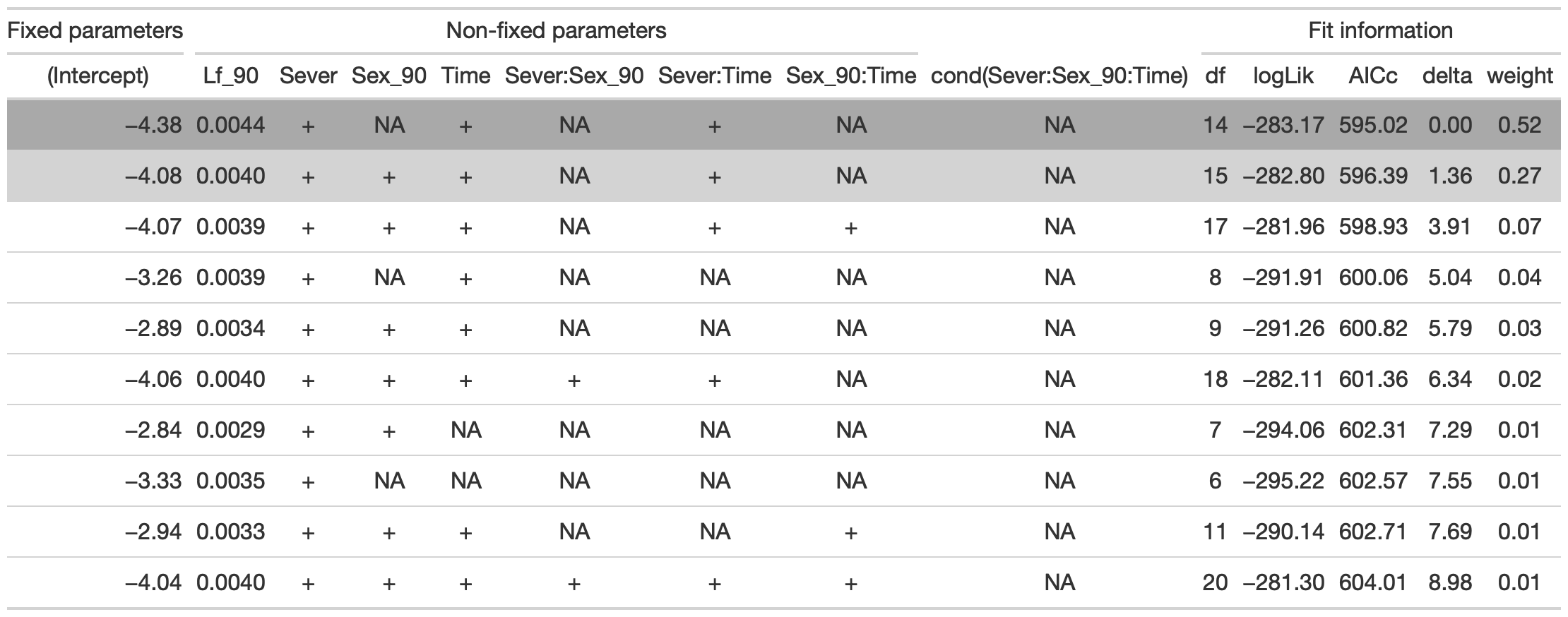
From this round of model selection, when Lf_90 is not required to be in the models that are considered, the same two models are returned as above.
3.3.4 Conclusion
mod_91brf_bm<-glmmTMB(branchingBinary~ Sever * Time + Lf_90 + (1|COLONY), data = mayappleAliveData,
                family="binomial")
The best and simplest model has main effects of Sever, Time, and Leaf area in 1990, and the Sever x Time interaction.
3.3.5 Estimated marginal means
Below are the relevant visualizations of the best model:
the sever x time interaction
g1 <- ggplot(data=mayappleAliveData, aes(x=Sever, y=branchingBinary, fill=Time)) +
  geom_bar(stat="summary", fun.y = "mean", position = "dodge") +
  ylab("Mean of binary response for\n not branching/branching ")

emmeans(mod_91brf_bm, pairwise~Time|Sever, type="response")
## $emmeans
## Sever = C:
## Time prob SE df lower.CL upper.CL
## T1 0.1016 0.0419 606 0.0439 0.218
## T2 0.2183 0.0605 606 0.1222 0.359
## T3 0.1636 0.0528 606 0.0840 0.294
##
## Sever = S1:
## Time prob SE df lower.CL upper.CL
## T1 0.5734 0.0868 606 0.4010 0.730
## T2 0.2444 0.0694 606 0.1339 0.403
## T3 0.1505 0.0510 606 0.0749 0.280
##
## Sever = S2:
## Time prob SE df lower.CL upper.CL
## T1 0.2294 0.0690 606 0.1215 0.391
## T2 0.1635 0.0553 606 0.0811 0.302
## T3 0.1642 0.0524 606 0.0849 0.294
##
## Sever = S4:
## Time prob SE df lower.CL upper.CL
## T1 0.1075 0.0463 606 0.0447 0.237
## T2 0.1404 0.0491 606 0.0684 0.266
## T3 0.0486 0.0256 606 0.0169 0.132
##
## Confidence level used: 0.95
## Intervals are back-transformed from the logit scale
##
## $contrasts
## Sever = C:
## contrast odds.ratio SE df t.ratio p.value
## T1 / T2 0.405 0.220 606 -1.662 0.2209
## T1 / T3 0.578 0.324 606 -0.977 0.5916
## T2 / T3 1.428 0.693 606 0.733 0.7440
##
## Sever = S1:
## contrast odds.ratio SE df t.ratio p.value
## T1 / T2 4.156 2.042 606 2.899 0.0108
## T1 / T3 7.584 3.883 606 3.957 0.0002
## T2 / T3 1.825 0.928 606 1.182 0.4642
##
## Sever = S2:
## contrast odds.ratio SE df t.ratio p.value
## T1 / T2 1.523 0.807 606 0.795 0.7064
## T1 / T3 1.515 0.778 606 0.809 0.6973
## T2 / T3 0.995 0.513 606 -0.010 0.9999
##
## Sever = S4:
## contrast odds.ratio SE df t.ratio p.value
## T1 / T2 0.738 0.441 606 -0.509 0.8672
## T1 / T3 2.361 1.652 606 1.228 0.4372
## T2 / T3 3.199 2.057 606 1.809 0.1674
##
## P value adjustment: tukey method for comparing a family of 3 estimates
## Tests are performed on the log odds ratio scale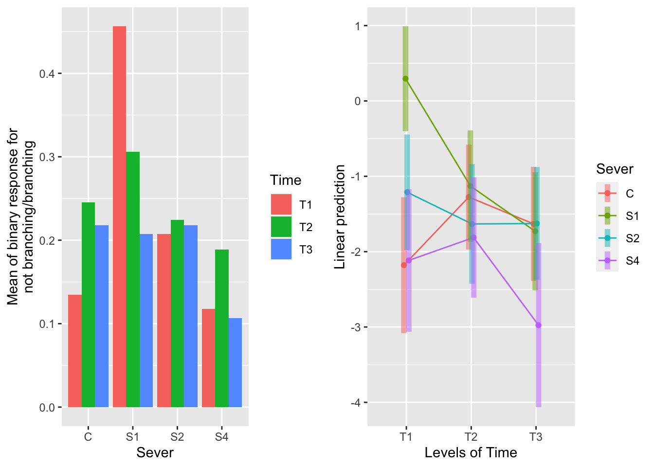
For T1 (in red on the raw data plot on the left), S1 systems are significantly more likely to branch than all other systems. In the emmeans plot on the right, we can see that the green bar for S1 at T1 is distinct from the other three severing treatment. The chances of branching do not vary across other times of severing.
the main effect of time
g1 <- ggplot(data=mayappleAliveData, aes(x=Time, y=branchingBinary)) +
  geom_bar(stat="summary", fun.y = "mean", position = "dodge") +
  ylab("Mean of binary response for\n not branching/branching ")

emmeans(mod_91brf_bm, pairwise~Time, type="response")
## $emmeans
## Time prob SE df lower.CL upper.CL
## T1 0.214 0.0404 606 0.1448 0.304
## T2 0.188 0.0350 606 0.1288 0.266
## T3 0.120 0.0273 606 0.0759 0.185
##
## Results are averaged over the levels of: Sever
## Confidence level used: 0.95
## Intervals are back-transformed from the logit scale
##
## $contrasts
## contrast odds.ratio SE df t.ratio p.value
## T1 / T2 1.17 0.319 606 0.585 0.8281
## T1 / T3 1.99 0.591 606 2.318 0.0541
## T2 / T3 1.70 0.462 606 1.941 0.1281
##
## Results are averaged over the levels of: Sever
## P value adjustment: tukey method for comparing a family of 3 estimates
## Tests are performed on the log odds ratio scale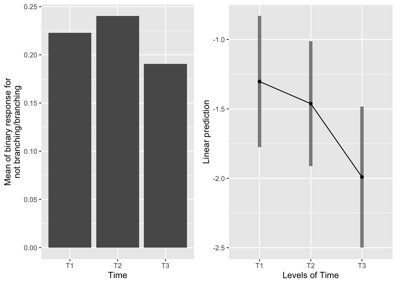
Likelihood of branching generally decreases from T1 to T2 to T3, but only the contrast between T1 and T3 is marginally significant; all others are non-significant.
the main effect of sever
g1 <- ggplot(data=mayappleAliveData, aes(x=Sever, y=branchingBinary)) +
  geom_bar(stat="summary", fun.y = "mean", position = "dodge") +
  ylab("Mean of binary response for\n not branching/branching ")

emmeans(mod_91brf_bm, pairwise~Sever, type="response")
## $emmeans
## Sever prob SE df lower.CL upper.CL
## C 0.155 0.0341 606 0.0992 0.234
## S1 0.298 0.0502 606 0.2100 0.405
## S2 0.184 0.0380 606 0.1206 0.270
## S4 0.091 0.0255 606 0.0518 0.155
##
## Results are averaged over the levels of: Time
## Confidence level used: 0.95
## Intervals are back-transformed from the logit scale
##
## $contrasts
## contrast odds.ratio SE df t.ratio p.value
## C / S1 0.431 0.128 606 -2.823 0.0253
## C / S2 0.814 0.246 606 -0.679 0.9051
## C / S4 1.833 0.625 606 1.777 0.2856
## S1 / S2 1.889 0.552 606 2.176 0.1312
## S1 / S4 4.250 1.436 606 4.280 0.0001
## S2 / S4 2.250 0.763 606 2.392 0.0796
##
## Results are averaged over the levels of: Time
## P value adjustment: tukey method for comparing a family of 4 estimates
## Tests are performed on the log odds ratio scale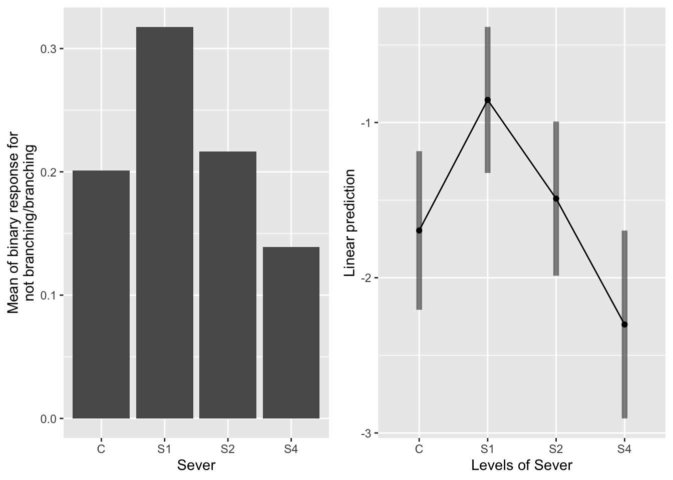
When pooling across the timing of severing, systems severed at S1 are more likely to branch than conrol or S4 systems. S1 and S2 actually aren’t significantly different.
the main effect of leaf area
newdat <- expand.grid(Lf_90=seq(min(mayappleAliveData$Lf_90,na.rm=TRUE), max(mayappleAliveData$Lf_90,na.rm=TRUE),len=100),
Sex_90=c("S","V"),
Time = c("T1","T2","T3"),
Sever = c("C","S1","S2","S4"),
COLONY = mayappleAliveData$COLONY)
newdat$brBinary = predict(mod_91brf_bm, newdata=newdat, type="response",re.form=~0)
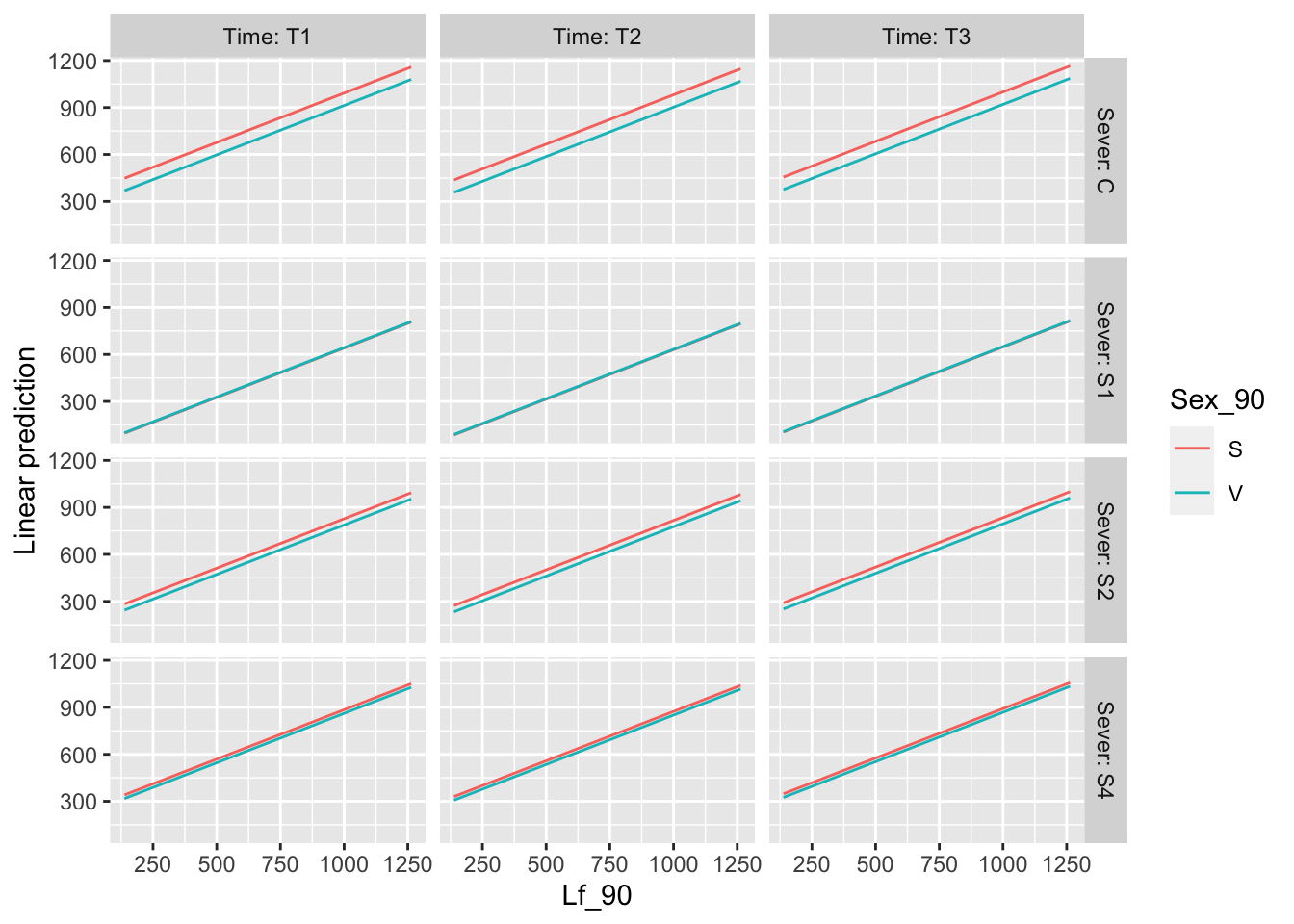
ggplot(data=mayappleAliveData, aes(x=Lf_90, y=branchingBinary, color=Sever)) +
geom_point() + geom_line(data=newdat, aes(x=Lf_90, y=brBinary, color=Sever))+
facet_wrap(~Time) +
ylab("Mean of binary response for\n not branching/branching ") 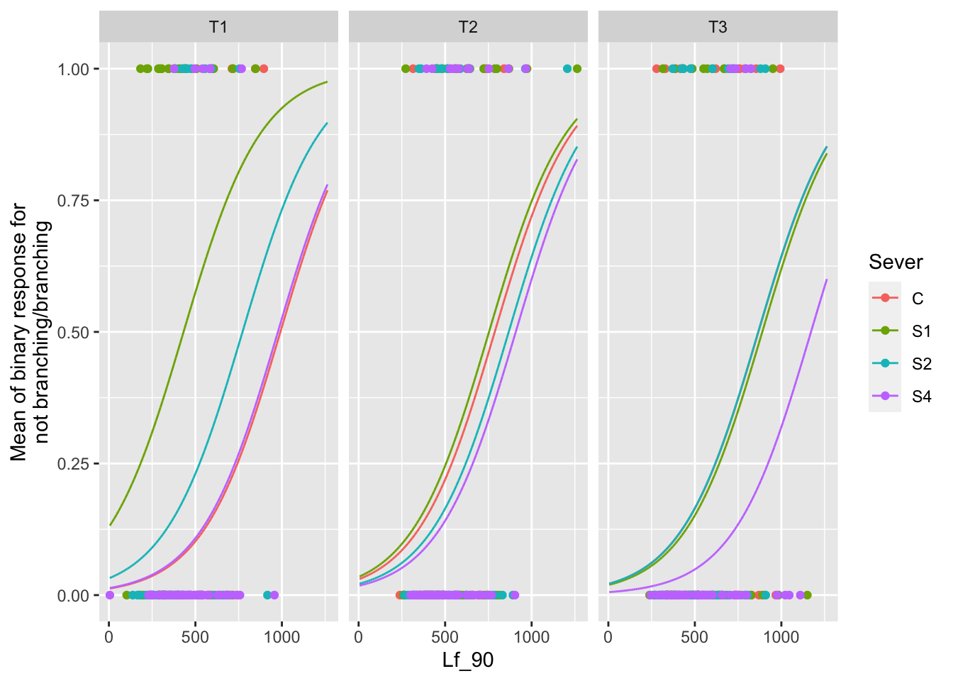
3.4 Sexual status
These analyses use systems that were alive in 1991; e.g., they had 1 or more branches. We are analyzing whether a system was sexual (had one or more sexual branches) or not (all branches were vegetative).
3.4.1 Data & visualization
# filter dataset to plants that have 1 or more branches
# recode the branch sex variables so that for each branch
# a vegetative branch is recorded as a 0
# a sexual branch is recorded as a 0
# sum across the rows to total the number of sexual branches
mayappleSexData <- mayappleDatasetFull %>%
  filter(!is.na(Lf_90)) %>%
  dplyr::filter(brnoF_91==1|brnoF_91==2|brnoF_91==3) %>%
  dplyr::mutate(SexF1_91 = as.numeric(ifelse(SexF1_91=="V",0,1)),
                SexF2_91 = as.numeric(ifelse(SexF2_91=="V",0,1)),
                SexF3_91 = as.numeric(ifelse(SexF3_91=="V",0,1))) %>%
  dplyr::rowwise() %>%
  dplyr::mutate(numberSexualBranches = sum(SexF1_91, SexF2_91, SexF3_91,na.rm=TRUE))

mayappleSexData$SexBr<-0
mayappleSexData$SexBr[mayappleSexData$numberSexualBranches==1|mayappleSexData$numberSexualBranches==2]<-1


ggplot(data=mayappleSexData, aes(x=Sever, y=numberSexualBranches, fill = Time)) +
  stat_summary(fun = mean, geom = "bar",position="dodge") +
  stat_summary(fun.data = mean_se, geom = "errorbar", position="dodge")+
  facet_wrap(~Sex_90) +
  ylab("Mean of binary variable for number of sexual branches\n per plant") +
  scale_fill_brewer(palette="Set1")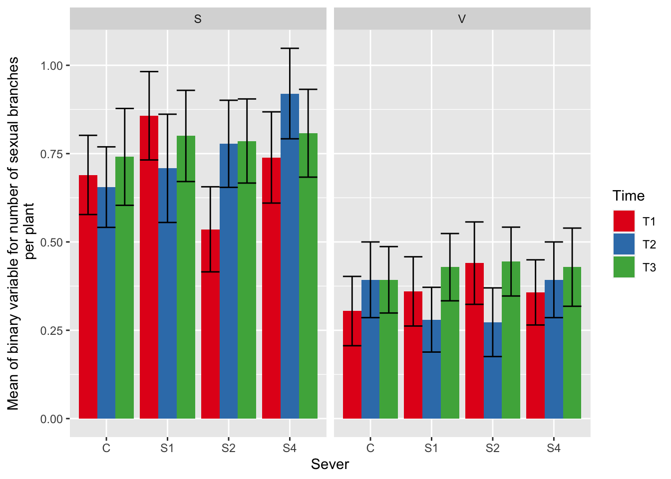
3.4.2 Model selection with leaf area
mod91sex0l<-glmmTMB(SexBr~ Sex_90*Sever *Time + Lf_90 + (1|COLONY), data = mayappleSexData,
                family="binomial")
#this is the global model
#MuMIn::getAllTerms(mod91sex0l) #this lets us see how to specify terms in the model

dr<-dredge(mod91sex0l, fixed=~cond(Lf_90))

tab <- head(dr, n=10) %>% gt() %>% cols_hide(columns=vars(`disp((Int))`)) %>%
  cols_label(`cond((Int))`="(Intercept)", `cond(Lf_90)`="Lf_90", `cond(Sever)`="Sever", `cond(Sex_90)`="Sex_90", `cond(Time)`="Time", `cond(Sever:Sex_90)`="Sever:Sex_90", `cond(Sever:Time)`="Sever:Time", `cond(Sex_90:Time)`= "Sex_90:Time") %>%
  fmt_number(columns = vars(`cond((Int))`, logLik, AICc, delta, weight), decimals = 2) %>%
  fmt_number(columns = vars(`cond(Lf_90)`), decimals = 4) %>%
  tab_spanner(label = "Fit information", columns = vars(df, logLik, AICc, delta, weight)) %>%
  tab_spanner(label = "Non-fixed parameters", columns = vars(`cond((Int))`,  `cond(Lf_90)`, `cond(Sever)`, `cond(Sex_90)`, `cond(Time)`, `cond(Sever:Sex_90)`, `cond(Sever:Time)`, `cond(Sex_90:Time)`)) %>%
  tab_spanner(label = "Fixed parameters", columns = vars(`cond((Int))`,  `cond(Lf_90)`)) %>%
    tab_style(style = cell_fill(color = "lightgrey"), locations = cells_body(columns = everything(),rows = delta <= 2)) %>%
  tab_style(style = cell_fill(color = "darkgrey"), locations = cells_body( columns = everything(), rows = 1))


tab %>% gtsave("front_91_sex_a.png", vwidth=1200) 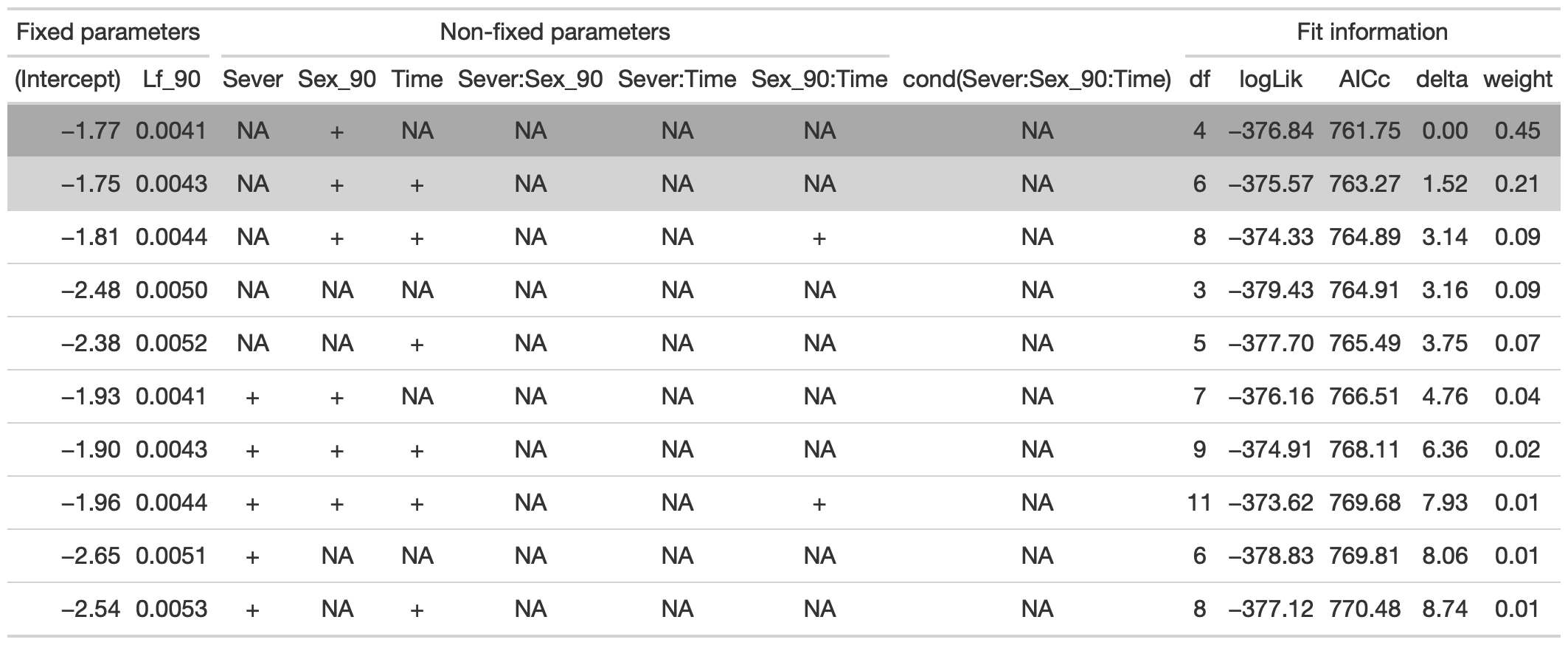
From this round of model selection, when Lf_90 is required to be in the models that are considered, there are two models within 2 AICc units: (1) Lf_90 and Sex_90 (AICc 761.7); (2) Lf_90, Sex_90, and Time (AICc 763.3).
3.4.3 Model selection without leaf area
dr<-dredge(mod91sex0l)

tab <- head(dr, n=10) %>% gt() %>% cols_hide(columns=vars(`disp((Int))`)) %>%
  cols_label(`cond((Int))`="(Intercept)", `cond(Lf_90)`="Lf_90", `cond(Sever)`="Sever", `cond(Sex_90)`="Sex_90", `cond(Time)`="Time", `cond(Sever:Sex_90)`="Sever:Sex_90", `cond(Sever:Time)`="Sever:Time", `cond(Sex_90:Time)`= "Sex_90:Time") %>%
  fmt_number(columns = vars(`cond((Int))`, logLik, AICc, delta, weight), decimals = 2) %>%
  fmt_number(columns = vars(`cond(Lf_90)`), decimals = 4) %>%
  tab_spanner(label = "Fit information", columns = vars(df, logLik, AICc, delta, weight)) %>%
  tab_spanner(label = "Non-fixed parameters", columns = vars(`cond((Int))`,  `cond(Lf_90)`, `cond(Sever)`, `cond(Sex_90)`, `cond(Time)`, `cond(Sever:Sex_90)`, `cond(Sever:Time)`, `cond(Sex_90:Time)`)) %>%
  tab_spanner(label = "Fixed parameters", columns = vars(`cond((Int))`, )) %>%
    tab_style(style = cell_fill(color = "lightgrey"), locations = cells_body(columns = everything(),rows = delta <= 2)) %>%
  tab_style(style = cell_fill(color = "darkgrey"), locations = cells_body( columns = everything(), rows = 1))


tab %>% gtsave("front_91_sex_b.png", vwidth=1200)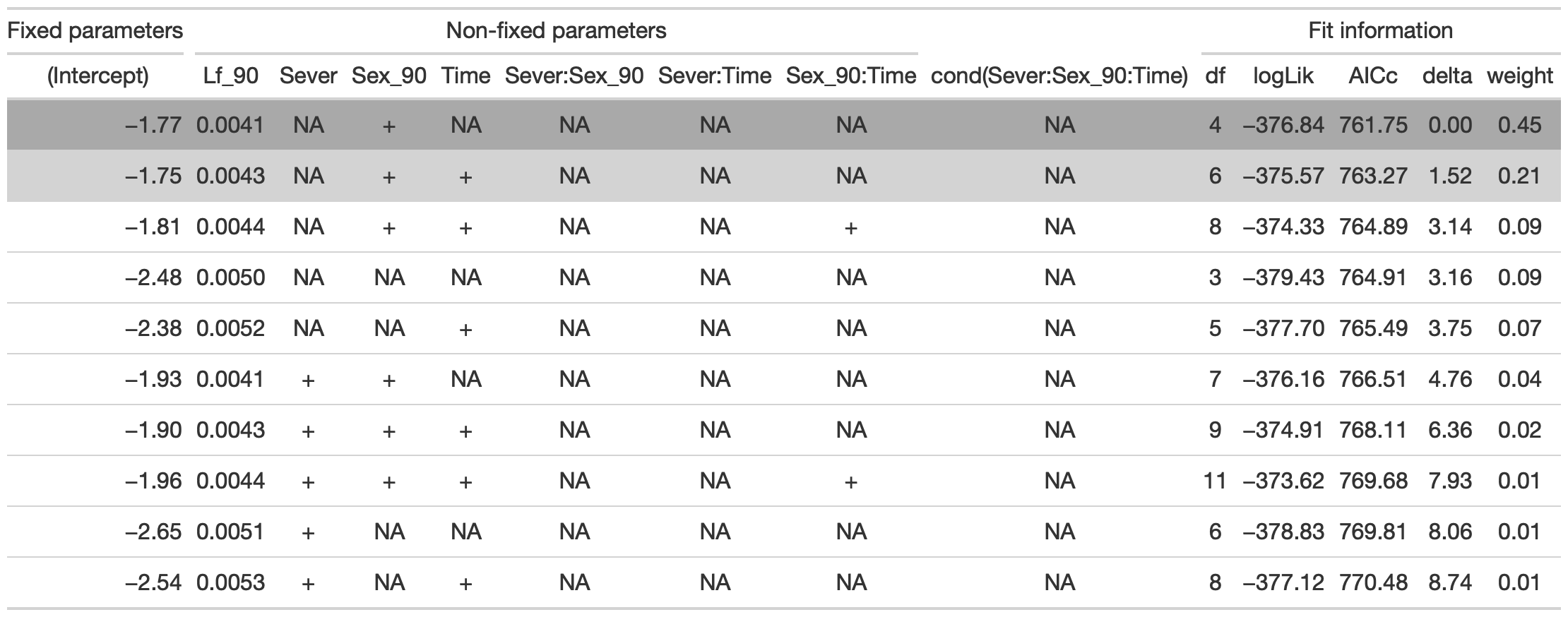
From this round of model selection, when Lf_90 is not required to be in the models that are considered, the same two models are returned as above.
3.4.4 Conclusion
The simplest model with the lowest AICc has main effects of Lf_90 and Sex_90.
3.4.5 Estimated marginal means
the main effect of sex
g1 <- ggplot(data=mayappleSexData, aes(x=Sex_90, y=SexBr)) +
  geom_bar(stat="summary", fun.y = "mean", position = "dodge") +
  ylab("Mean of binary variable for having zero vs. one or more sexual shoots")

emmeans(mod91sexbm, pairwise~Sex_90, type="response")
## $emmeans
## Sex_90 prob SE df lower.CL upper.CL
## S 0.567 0.0496 616 0.468 0.661
## V 0.442 0.0506 616 0.346 0.543
##
## Confidence level used: 0.95
## Intervals are back-transformed from the logit scale
##
## $contrasts
## contrast odds.ratio SE df t.ratio p.value
## S / V 1.65 0.364 616 2.281 0.0229
##
## Tests are performed on the log odds ratio scale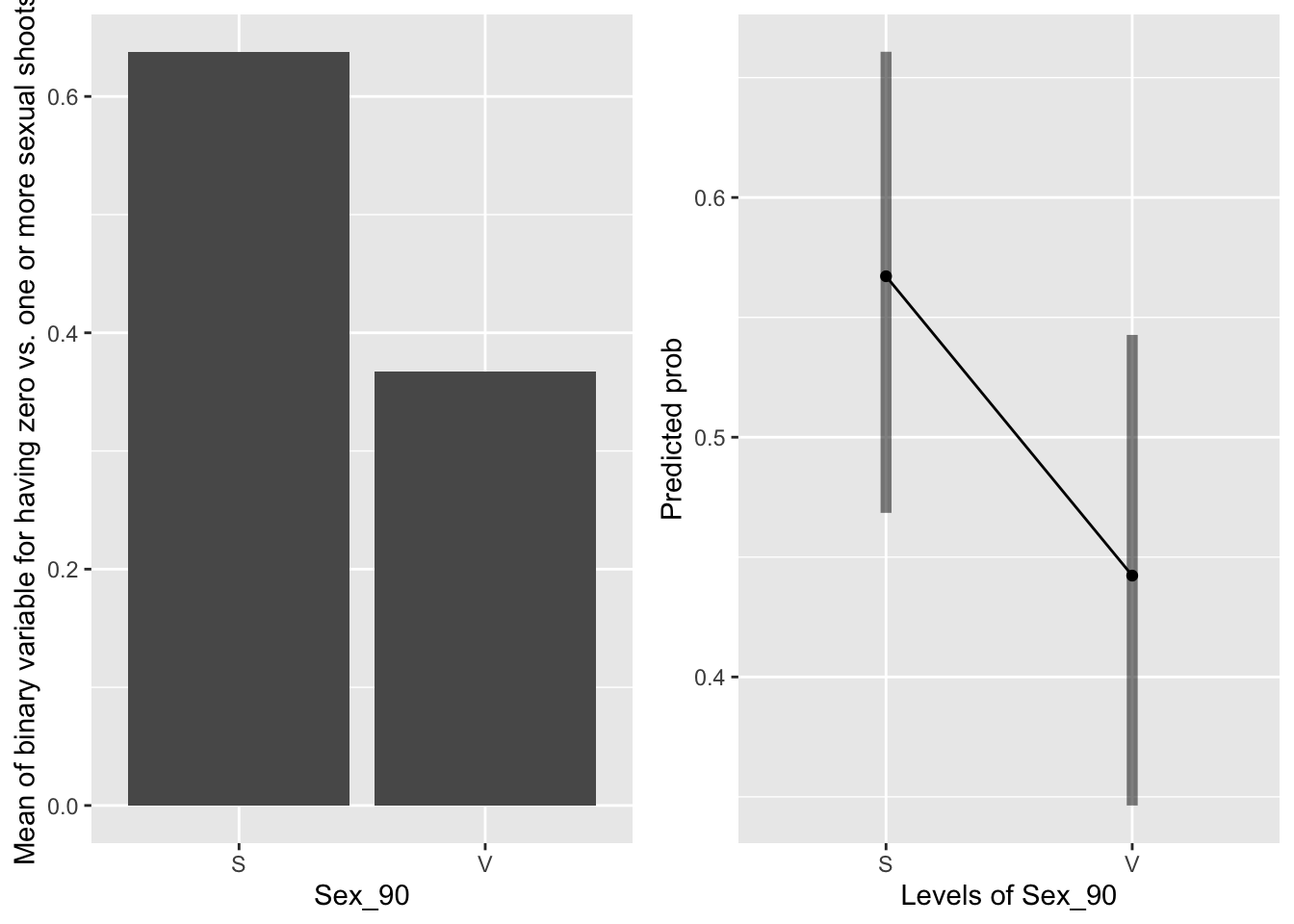
Systems that were sexual in 1990 are much more likely to be sexual in 1991.
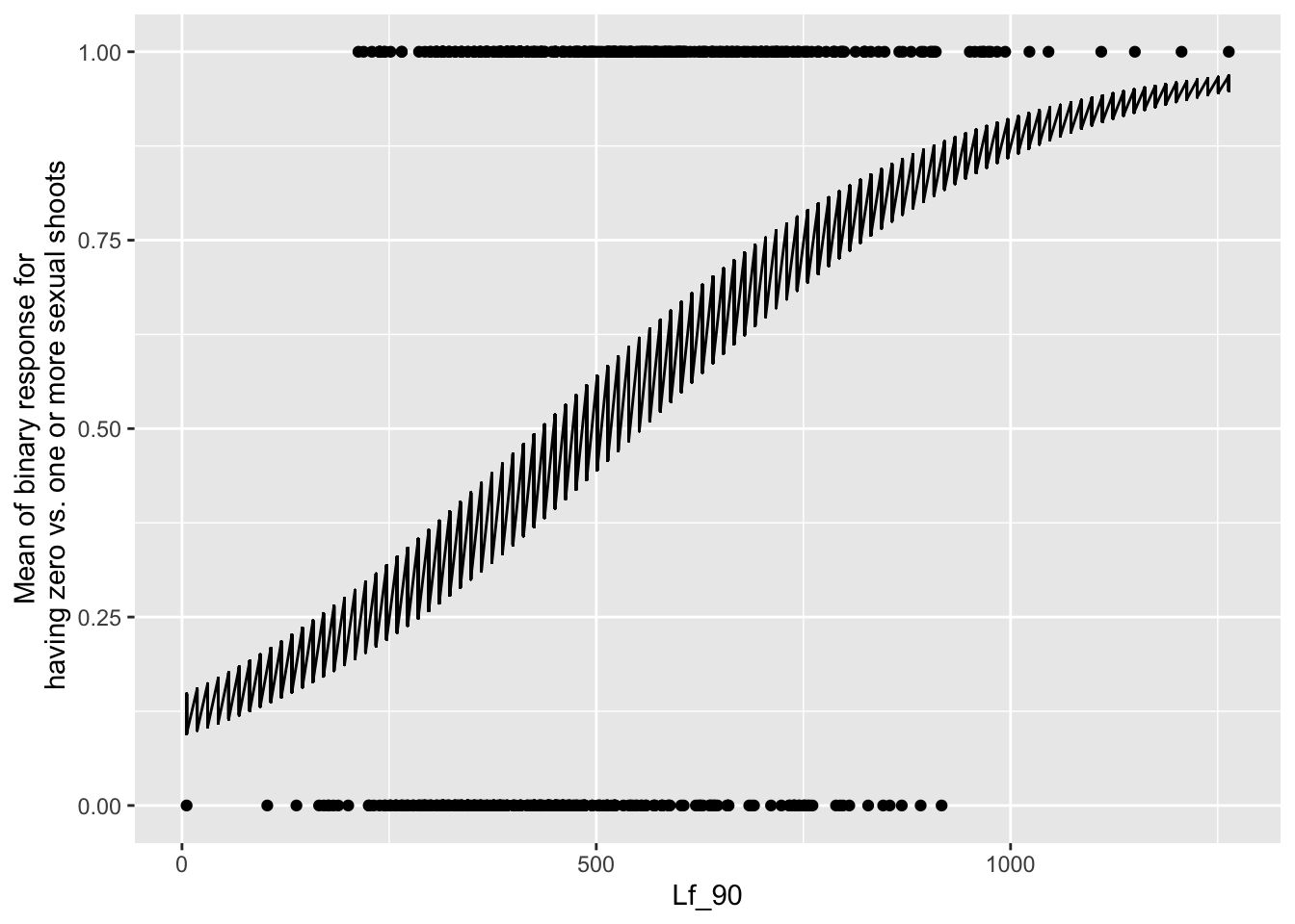
the main effect of leaf area
newdat <- expand.grid(Lf_90=seq(min(mayappleSexData$Lf_90,na.rm=TRUE), max(mayappleSexData$Lf_90,na.rm=TRUE),len=100),
                     Sex_90=c("S","V"),
                     COLONY = mayappleSexData$COLONY)
newdat$brBinary = predict(mod91sexbm, newdata=newdat, type="response",re.form=~0)

ggplot(data=mayappleSexData, aes(x=Lf_90, y=SexBr)) +
  geom_point() + geom_line(data=newdat, aes(x=Lf_90, y=brBinary))+
  ylab("Mean of binary response for\n having zero vs. one or more sexual shoots")