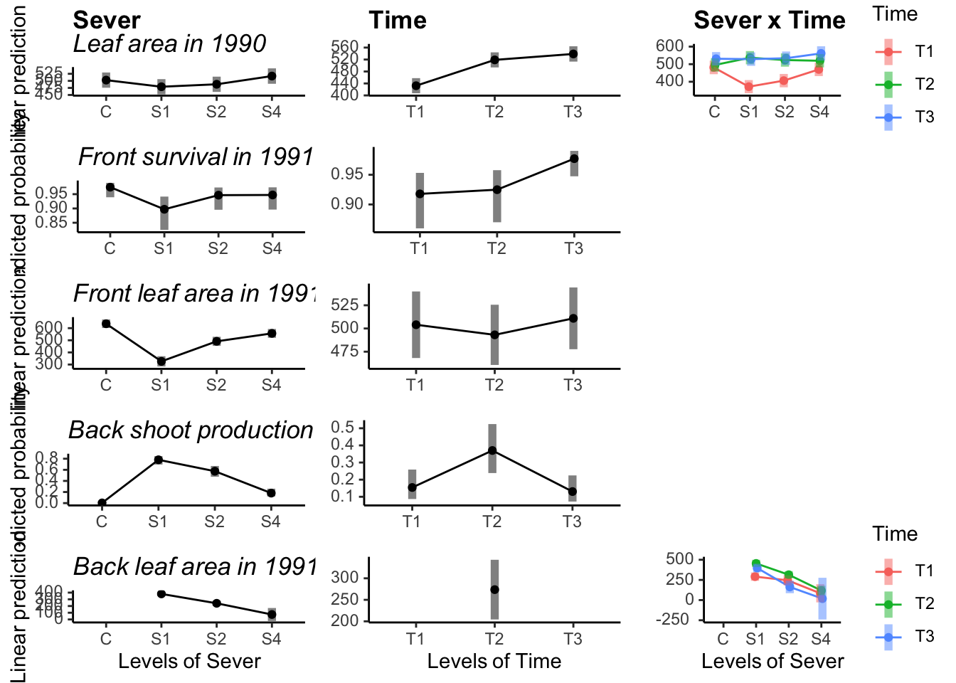
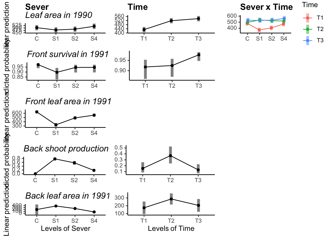
10 Multipanel figure for MS

10.1 Goals:

Pull code for the following models together into one place:

• Leaf area in 1990
• Front survival in 1991
• Front leaf area in 1991
• Back shoot production in 1991
• Back leaf area in 1991

Then, using that code, make the following figure panels:

Response	Sever	Time	Interaction
Leaf 1990	Yes	Yes	Yes
Front survival 1991	Yes	Yes
Front leaf area 1991	Yes	Yes
Back shoot production 1991	Yes	Yes
Back leaf area 1991	Yes	Yes	Yes

Then, put all of those panels into one 5 x 3 grid!

10.2 Leaf area in 1990

may<-read.csv("Datasets/mayapple_1990_updated.csv")
##need to make the variables we are working with numeric:
may$Lf_90<-as.numeric(as.character(may$Lf_90))

may<-may %>% 
  filter(!is.na(Lf_90))

10.2.1 Best model

model.bm<-lmer(Lf_90~Sex_90*Time+Sever*Time+(1|COLONY), data=may, na.action = "na.fail", REML=FALSE)

The best model includes fixed effects of Sever, Sex_90, Time, the Sever x Time interaction, and the Sex_90 x Time interaction.

10.2.2 Estimated marginal means

The main effect of Sever:

#emmeans(model.bm, pairwise~Sever, type="response")
library(mdthemes)

Sever_1 <- emmip(model.bm,  ~ Sever ,CIs = TRUE)+xlab("")+mdthemes::md_theme_classic() +ggtitle("**Sever**  
                                                                                                         *Leaf area in 1990*")

The main effect of Time:

#emmeans(model.bm, pairwise~Time, type="response")

Time_1 <- emmip(model.bm,  ~ Time ,CIs = TRUE)+xlab("")+ylab("")+mdthemes::md_theme_classic() +ggtitle("**Time**")                                                                                                  

The Sever x Time interaction:

#emmeans(model.bm, pairwise~Time|Sever, type="response")
Int_1 <- emmip(model.bm, Time  ~ Sever  ,CIs = TRUE)+xlab("")+ylab("")+mdthemes::md_theme_classic()+ggtitle("**Sever x Time**")

10.3 Front survival 1991

# set na.strings="." to recode '.' to NA
mayappleDatasetFull<-readxl::read_excel("Datasets/mayapple_1990_updated.xlsx", na=".")

# select variables for analysis and filter out rows that don't have a leaf area recorded in 1990
mayappleData <- mayappleDatasetFull %>% 
  dplyr::select(COLONY,Lf_90,brnoF_91,Sex_90,Sever,Time,SexF1_91,SexF2_91,SexF3_91,LfFtot_91) %>% 
  filter(!is.na(Lf_90))

# create binary variable for plants that are dead/have no branches (0) or have 1 or more branches (1)
# append new variable to the dataframe
mayappleData<- mayappleData %>% 
  dplyr::mutate(deadAliveBinary=ifelse(brnoF_91>0,1,0))

10.3.1 Best model

sur_91f_bm<-glmmTMB(deadAliveBinary~ Sever+Time +  (1|COLONY), data = mayappleData,
                family="binomial")

10.3.2 Estimated marginal means

The main effect of severing

#emmeans(sur_91f_bm, pairwise~Sever, type="response" )

Sever_2 <- emmip(sur_91f_bm,   ~ Sever  , type="response",CIs = TRUE)+xlab("")+ylab("Predicted probability")+mdthemes::md_theme_classic()+ggtitle("*Front survival in 1991*")

The main effect of time

#emmeans(sur_91f_bm, pairwise~Time, type="response" )

Time_2 <- emmip(sur_91f_bm,   ~ Time  ,type="response",CIs = TRUE)+xlab("")+ylab("")+mdthemes::md_theme_classic()

10.4 Front conditional leaf area 1991

mayappleData$LfFtot_91<-as.numeric(mayappleData$LfFtot_91)

mayappleData <- mayappleData %>% 
  filter(!is.na(LfFtot_91)) %>% 
  filter(LfFtot_91>0)

10.4.1 Best model

mod91laf.bm<-lmer(LfFtot_91~Sever+Lf_90 +(1|COLONY), data = mayappleData, na.action ="na.fail", REML=FALSE)

10.4.2 Estimated marginal means

the main effect of sever

#emmeans(mod91laf.bm, pairwise~Sever, type="response")

Sever_3cond <- emmip(mod91laf.bm,   ~ Sever  ,CIs = TRUE)+xlab("")+mdthemes::md_theme_classic()+ggtitle("*Front leaf area in 1991*")

10.5 Front leaf area 1991

mayappleData$LfFtot_91<-as.numeric(mayappleData$LfFtot_91)

mayappleData <- mayappleData %>% 
  filter(!is.na(LfFtot_91))

10.5.1 Best model

mod91laf.bm<-lmer(LfFtot_91~Sex_90*Sever+Time+Lf_90 +(1|COLONY), data = mayappleData, na.action ="na.fail", REML=FALSE)

10.5.2 Estimated marginal means

the main effect of sever

#emmeans(mod91laf.bm, pairwise~Sever, type="response")

Sever_3 <- emmip(mod91laf.bm,   ~ Sever  ,CIs = TRUE)+xlab("")+mdthemes::md_theme_classic()+ggtitle("*Front leaf area in 1991*")

Control systems have the most leaf area. S1 systems have the least leaf area. S2 and S4 systems are intermediate and not different from each other.

the main effect of time

#emmeans(mod91laf.bm, pairwise~Time, type="response")

Time_3 <- emmip(mod91laf.bm,   ~ Time  ,CIs = TRUE)+xlab("")+ylab("")+mdthemes::md_theme_classic()

10.6 Back shoot production 1991

# set na.strings="." to recode '.' to NA
mayappleDatasetFull<-readxl::read_excel("Datasets/mayapple_1990_updated.xlsx", na=".")

mayappleData <- mayappleDatasetFull %>% 
  dplyr::select(COLONY,Lf_90,Sex_90,Sever,Time,brnoB_91,LfB1_91,SexB1_91,LfB2_91,SexB2_91,LfBtot_91,Lftot_91) %>% 
  filter(!is.na(Lf_90))

mayappleData<- mayappleData %>% 
  dplyr::mutate(backShootBranchBinary=ifelse(brnoB_91>0,1,0)) %>% 
  filter(!is.na(backShootBranchBinary))

10.6.1 Best model

sur_91b_bm<-glmmTMB(backShootBranchBinary~ Sever+Time + Lf_90 +(1|COLONY), data = mayappleData,
                family="binomial")

10.6.2 Estimated marginal means

The main effect of severing

#emmeans(sur_91b_bm, pairwise~Sever, type="response" )

Sever_4 <- emmip(sur_91b_bm,   ~ Sever  ,type="response",CIs = TRUE )+xlab("")+ylab("Predicted probability")+mdthemes::md_theme_classic()+ggtitle("*Back shoot production in 1991*")

The main effect of time

#emmeans(sur_91b_bm, pairwise~Time, type="response" )

Time_4 <- emmip(sur_91b_bm,   ~ Time  ,type="response",CIs = TRUE )+xlab("")+ylab("")+mdthemes::md_theme_classic()

10.7 Back conditional leaf area 1991

mayappleData$LfBtot_91<-as.numeric(mayappleData$LfBtot_91)

## Warning: NAs introduced by coercion

mayappleData <- mayappleData %>% 
  filter(!is.na(LfBtot_91)) %>% 
  filter(LfBtot_91>0)

10.7.1 Best model

b_mod91la.bm<-lmer(LfBtot_91~Sex_90+Sever+Time +Lf_90+(1|COLONY), data = mayappleData, na.action ="na.fail", REML=FALSE)

10.7.2 Estimated marginal means

the main effect of sever

#emmeans(b_mod91la.bm, pairwise~Sever, type="response")

Sever_5cond <- emmip(b_mod91la.bm,  ~ Sever  ,CIs = TRUE )+mdthemes::md_theme_classic()+ggtitle("*Back leaf area in 1991*")

## Cannot use mode = "kenward-roger" because *pbkrtest* package is not installed

#emmeans(b_mod91la.bm, pairwise~Time, type="response")

Time_5cond <- emmip(b_mod91la.bm,  ~ Time  ,CIs = TRUE )+ylab("")+mdthemes::md_theme_classic()

## Cannot use mode = "kenward-roger" because *pbkrtest* package is not installed

10.8 Back leaf area 1991

mayappleData$LfBtot_91<-as.numeric(mayappleData$LfBtot_91)

mayappleData <- mayappleData %>% 
  filter(!is.na(LfBtot_91))

10.8.1 Best model

b_mod91la.bm<-lmer(LfBtot_91~Sex_90*Sever+Sever*Time +Lf_90+(1|COLONY), data = mayappleData, na.action ="na.fail", REML=FALSE)

## fixed-effect model matrix is rank deficient so dropping 3 columns / coefficients

10.8.2 Estimated marginal means

the main effect of sever

#emmeans(b_mod91la.bm, pairwise~Sever, type="response")

Sever_5 <- emmip(b_mod91la.bm,  ~ Sever  ,CIs = TRUE )+mdthemes::md_theme_classic()+ggtitle("*Back leaf area in 1991*")

## Cannot use mode = "kenward-roger" because *pbkrtest* package is not installed

## NOTE: Results may be misleading due to involvement in interactions

the main effect of time

#emmeans(b_mod91la.bm, pairwise~Time, type="response")

Time_5 <- emmip(b_mod91la.bm,  ~ Time  ,CIs = TRUE )+ylab("")+mdthemes::md_theme_classic()

## Cannot use mode = "kenward-roger" because *pbkrtest* package is not installed

## NOTE: Results may be misleading due to involvement in interactions

the sever x time interaction

#emmeans(b_mod91la.bm, pairwise~Time|Sever, type="response")

Int_5 <- emmip(b_mod91la.bm, Time  ~ Sever  ,CIs = TRUE )+ylab("")+mdthemes::md_theme_classic()

## Cannot use mode = "kenward-roger" because *pbkrtest* package is not installed

10.9 Multipanel figure

library("cowplot")

ggdraw() +
  draw_plot(Sever_1, x=0, y=0.8, width=0.33, height=0.2)+
  draw_plot(Sever_2, x=0, y=0.6,width=0.33, height=0.2)+
  draw_plot(Sever_3, x=0, y=0.4,width=0.33, height=0.2)+
  draw_plot(Sever_4, x=0, y=0.2,width=0.33, height=0.2)+
  draw_plot(Sever_5, x=0, y=0.0,width=0.33, height=0.2)+
  draw_plot(Time_1, x=0.33, y=0.8, width=0.33, height=0.2)+
  draw_plot(Time_2, x=0.33, y=0.6,width=0.33, height=0.2)+
  draw_plot(Time_3, x=0.33, y=0.4,width=0.33, height=0.2)+
  draw_plot(Time_4, x=0.33, y=0.2,width=0.33, height=0.2)+
  draw_plot(Time_5, x=0.33, y=0.0,width=0.33, height=0.2)+
  draw_plot(Int_1, x=0.67, y=0.8, width=0.33, height=0.2)+
  draw_plot(Int_5, x=0.67, y=0.0, width=0.33, height=0.2)

#For conditional leaf area:

ggdraw() +
  draw_plot(Sever_1, x=0, y=0.8, width=0.33, height=0.2)+
  draw_plot(Sever_2, x=0, y=0.6,width=0.33, height=0.2)+
  draw_plot(Sever_3cond, x=0, y=0.4,width=0.33, height=0.2)+
  draw_plot(Sever_4, x=0, y=0.2,width=0.33, height=0.2)+
  draw_plot(Sever_5cond, x=0, y=0.0,width=0.33, height=0.2)+
  draw_plot(Time_1, x=0.33, y=0.8, width=0.33, height=0.2)+
  draw_plot(Time_2, x=0.33, y=0.6,width=0.33, height=0.2)+
  draw_plot(Time_4, x=0.33, y=0.2,width=0.33, height=0.2)+
  draw_plot(Time_5cond, x=0.33, y=0.0,width=0.33, height=0.2)+
  draw_plot(Int_1, x=0.67, y=0.8, width=0.33, height=0.2)