6 1992 front system analyses

6.1 Leaf area

This analysis uses all systems that have a non-NA value for total leaf area of the front and back in 1991 and in 1992, excluding those systems for which 1990 leaf area was NA.

6.1.1 Data & visualization

Read in data

# set na.strings="." to recode '.' to NA
mayappleDatasetFull<-readxl::read_excel("Datasets/mayapple_1990_updated_version2.xlsx", na=".")

Select the total leaf area in front in 1992 variable, and the independent variables. Also filtering out rows that don’t have a leaf area record in 1990. We need to do this in order to be able to compare models from model set A (which don’t include leaf area, and so wouldn’t naturally be affected by the missing data) with models from model set B (which do include leaf area and would be affected by the missing data). In other words, removing these rows means that model set A and model set B will run using the exact same dataset, which is necessary in order for us to compare the models.

# select variables for analysis and filter out rows that don't have a leaf area recorded in 1990
mayappleData <- mayappleDatasetFull %>% 
  dplyr::select(COLONY,Lf_90,Sex_90,Sever,Time,LftotF_92, Lftot_91, LfBtot_91, LfFtot_91) %>% 
  mutate(LftotF_92=parse_double(LftotF_92), Lftot_91=parse_double(Lftot_91), LfBtot_91=parse_double(LfBtot_91), LfFtot_91=parse_double(LfFtot_91) ) %>% 
  filter(!is.na(Lf_90)) %>% 
  filter(!is.na(Lftot_91)) %>% 
  filter(!is.na(LftotF_92))

ggplot(data=mayappleData, aes(x=Sever, y=LftotF_92, fill = Time)) +
   stat_summary(fun = mean, geom = "bar",position="dodge") + 
  stat_summary(fun.data = mean_se, geom = "errorbar", position="dodge")+
  facet_wrap(~Sex_90) +
  ylab("Mean total leaf area \n in front shoots in 1992") +
  scale_fill_brewer(palette="Set1")

6.1.2 Model selection with leaf area in 1990 and 1991

d_mod92la.0l<-lmer(LftotF_92~Sex_90*Sever*Time +LfFtot_91+Lf_90+(1|COLONY), data = mayappleData, na.action ="na.fail", REML=FALSE)


#this is the global model 
#MuMIn::getAllTerms(d_mod92la.0l) #this lets us see how to specify terms in the model

dr<-dredge(d_mod92la.0l, fixed=~Lf_90+LfFtot_91)

tab <- head(dr, n=10) %>% gt() %>%
  fmt_number(columns = vars(`(Intercept)`, Lf_90, LfFtot_91, logLik, AICc, delta, weight), decimals = 2) %>% 
  tab_spanner(label = "Fit information", columns = vars(df, logLik, AICc, delta, weight)) %>% 
  tab_spanner(label = "Non-fixed parameters", columns = vars(`(Intercept)`,   Lf_90, LfFtot_91, Sever, Sex_90, Time,  `Sever:Sex_90`, `Sever:Time`, `Sex_90:Time`, `Sever:Sex_90:Time`)) %>% 
  tab_spanner(label = "Fixed parameters", columns = vars(`(Intercept)`,Lf_90, LfFtot_91)) %>% 
    tab_style(style = cell_fill(color = "lightgrey"), locations = cells_body(columns = everything(),rows = delta <= 2)) %>% 
  tab_style(style = cell_fill(color = "darkgrey"), locations = cells_body( columns = everything(), rows = 1)) 
  

tab %>% gtsave("front_92_a.png", vwidth=1200)  

From this round of model selection, when Lf_90 and LfFtot_91 are required to be in the models that are considered, there are three models within two AICc units: (1) Lf_90, and LfF_91 (AICc 2924.1) (2) Lf_90, LfF_91, and Time (AICc 2925.1) (3) Lf_90, LfF_91, and Sex_90 (AICc 2926)

6.1.3 Model selection with leaf area in 1991

dr<-dredge(d_mod92la.0l, fixed=~LfFtot_91)

tab <- head(dr, n=10) %>% gt() %>%
  fmt_number(columns = vars(`(Intercept)`, Lf_90, LfFtot_91, logLik, AICc, delta, weight), decimals = 2) %>% 
  tab_spanner(label = "Fit information", columns = vars(df, logLik, AICc, delta, weight)) %>% 
  tab_spanner(label = "Non-fixed parameters", columns = vars(`(Intercept)`,   Lf_90, LfFtot_91, Sever, Sex_90, Time,  `Sever:Sex_90`, `Sever:Time`, `Sex_90:Time`, `Sever:Sex_90:Time`)) %>% 
  tab_spanner(label = "Fixed parameters", columns = vars(`(Intercept)`, LfFtot_91)) %>% 
    tab_style(style = cell_fill(color = "lightgrey"), locations = cells_body(columns = everything(),rows = delta <= 2)) %>% 
  tab_style(style = cell_fill(color = "darkgrey"), locations = cells_body( columns = everything(), rows = 1)) 
  

tab %>% gtsave("front_92_b.png", vwidth=1200)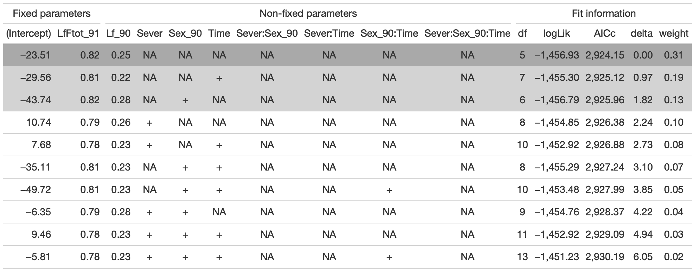  

From this round of model selection, when LfFtot_91 only is required to be in the models that are considered, the same three models are returned.

6.1.4 Model selection with leaf area in 1990

dr<-dredge(d_mod92la.0l, fixed=~Lf_90)

tab <- head(dr, n=10) %>% gt() %>%
  fmt_number(columns = vars(`(Intercept)`, Lf_90, LfFtot_91, logLik, AICc, delta, weight), decimals = 2) %>% 
  tab_spanner(label = "Fit information", columns = vars(df, logLik, AICc, delta, weight)) %>% 
  tab_spanner(label = "Non-fixed parameters", columns = vars(`(Intercept)`,   Lf_90, LfFtot_91, Sever, Sex_90, Time,  `Sever:Sex_90`, `Sever:Time`, `Sex_90:Time`, `Sever:Sex_90:Time`)) %>% 
  tab_spanner(label = "Fixed parameters", columns = vars(`(Intercept)`, Lf_90)) %>% 
    tab_style(style = cell_fill(color = "lightgrey"), locations = cells_body(columns = everything(),rows = delta <= 2)) %>% 
  tab_style(style = cell_fill(color = "darkgrey"), locations = cells_body( columns = everything(), rows = 1)) 
  

tab %>% gtsave("front_92_c.png", vwidth=1200)  

From this round of model selection, when Lf_90 is required to be in the models that are considered, the same three models are returned.

6.1.5 Model selection without leaf area

dr<-dredge(d_mod92la.0l)

## Fixed term is "(Intercept)"

tab <- head(dr, n=10) %>% gt() %>%
  fmt_number(columns = vars(`(Intercept)`, Lf_90, LfFtot_91, logLik, AICc, delta, weight), decimals = 2) %>% 
  tab_spanner(label = "Fit information", columns = vars(df, logLik, AICc, delta, weight)) %>% 
  tab_spanner(label = "Non-fixed parameters", columns = vars(`(Intercept)`,   Lf_90, LfFtot_91, Sever, Sex_90, Time,  `Sever:Sex_90`, `Sever:Time`, `Sex_90:Time`, `Sever:Sex_90:Time`)) %>% 
  tab_spanner(label = "Fixed parameters", columns = vars(`(Intercept)`)) %>% 
    tab_style(style = cell_fill(color = "lightgrey"), locations = cells_body(columns = everything(),rows = delta <= 2)) %>% 
  tab_style(style = cell_fill(color = "darkgrey"), locations = cells_body( columns = everything(), rows = 1)) 
  

tab %>% gtsave("front_92_d.png", vwidth=1200)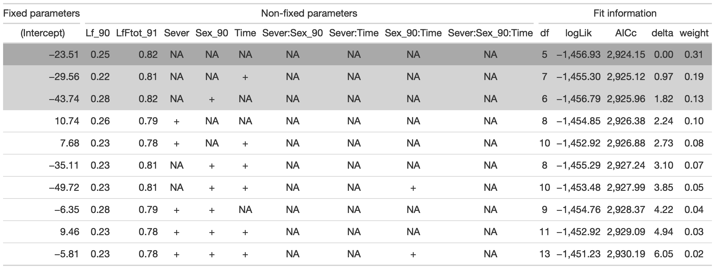  

From this round of model selection, when the leaf area effects are not required to be in the models that are considered, once again the same three models are returned.

6.1.6 Conclusion

d_mod92la.bm<-lmer(LftotF_92~+LfFtot_91+Lf_90+(1|COLONY), data = mayappleData, na.action ="na.fail")

The best model here contains fixed effects of leaf area in 1990 and 1991.

6.1.7 Estimated marginal means

the main effect of leaf area in 1990

mylist <- list(Lf_90=seq(150,1250,by=100))

g1 <- ggplot(data=mayappleData, aes(x=Lf_90, y=LftotF_92,color=Sever)) +
  geom_point(alpha=0.5) +
  ylab("Mean total leaf area \n in front shoots in 1992") 

g2 <- emmip(d_mod92la.bm,  ~ Lf_90 , at=mylist, CIs = TRUE)
gridExtra::grid.arrange(g1,g2,nrow=1)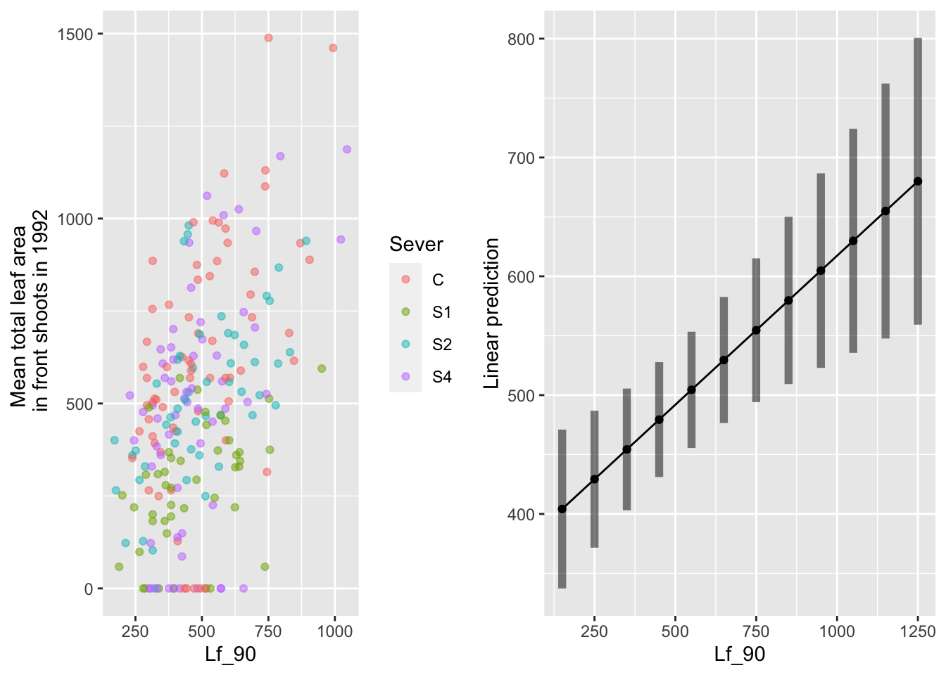

Of those systems that had non-zero leaf area in 1992, there is a positive relationship with leaf area in 1990.

the main effect of leaf area in 1991

mylist <- list(LfFtot_91=seq(0,1500,by=100))

g1 <- ggplot(data=mayappleData, aes(x=LfFtot_91, y=LftotF_92, color=Sever)) +
  geom_point(alpha=0.5) +
  ylab("Mean total leaf area \n in front shoots in 1992") 

g2 <- emmip(d_mod92la.bm,  ~ LfFtot_91 , at=mylist, CIs = TRUE)
gridExtra::grid.arrange(g1,g2,nrow=1)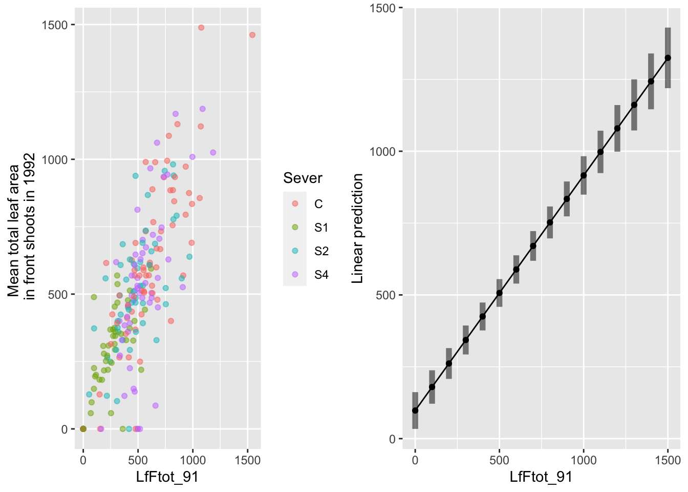

Aside from a small number of systems that had non-zero leaf area in 1991 and had zero leaf area in 1992, there is a positive relationship between leaf area in 1991 and 1992.

6.2 Conditional leaf area

This analysis uses all systems that have a non-NA value for total leaf area of the front and back in 1991 and in 1992, excluding those systems for which 1990 leaf area was NA. Furthermore, it restricts the analysis to those systems that have a non-zero leaf area in 1992.

6.2.1 Data & visualization

Read in data

# set na.strings="." to recode '.' to NA
mayappleDatasetFull<-readxl::read_excel("Datasets/mayapple_1990_updated_version2.xlsx", na=".")

Select the total leaf area in front in 1992 variable, and the independent variables. Also filtering out rows that don’t have a leaf area record in 1990. We need to do this in order to be able to compare models from model set A (which don’t include leaf area, and so wouldn’t naturally be affected by the missing data) with models from model set B (which do include leaf area and would be affected by the missing data). In other words, removing these rows means that model set A and model set B will run using the exact same dataset, which is necessary in order for us to compare the models.

# select variables for analysis and filter out rows that don't have a leaf area recorded in 1990
mayappleData <- mayappleDatasetFull %>% 
  dplyr::select(COLONY,Lf_90,Sex_90,Sever,Time,LftotF_92, Lftot_91, LfBtot_91, LfFtot_91) %>% 
  mutate(LftotF_92=parse_double(LftotF_92), Lftot_91=parse_double(Lftot_91), LfBtot_91=parse_double(LfBtot_91), LfFtot_91=parse_double(LfFtot_91) ) %>% 
  filter(!is.na(Lf_90)) %>% 
  filter(!is.na(Lftot_91)) %>% 
  filter(!is.na(LftotF_92)) %>% 
  filter(LftotF_92>0)

ggplot(data=mayappleData, aes(x=Sever, y=LftotF_92, fill = Time)) +
   stat_summary(fun = mean, geom = "bar",position="dodge") + 
  stat_summary(fun.data = mean_se, geom = "errorbar", position="dodge")+
  facet_wrap(~Sex_90) +
  ylab("Mean total leaf area \n in front shoots in 1992") +
  scale_fill_brewer(palette="Set1")

6.2.2 Model selection with leaf area in 1990 and 1991

d_mod92la.0l<-lmer(LftotF_92~Sex_90*Sever*Time +LfFtot_91+Lf_90+(1|COLONY), data = mayappleData, na.action ="na.fail", REML=FALSE)


#this is the global model 
#MuMIn::getAllTerms(d_mod92la.0l) #this lets us see how to specify terms in the model

dr<-dredge(d_mod92la.0l)

tab <- head(dr, n=10) %>% gt() %>%
  fmt_number(columns = vars(`(Intercept)`, Lf_90, LfFtot_91, logLik, AICc, delta, weight), decimals = 2) %>% 
  tab_spanner(label = "Fit information", columns = vars(df, logLik, AICc, delta, weight)) %>% 
  tab_spanner(label = "Non-fixed parameters", columns = vars(`(Intercept)`,   Lf_90, LfFtot_91, Sever, Sex_90, Time,  `Sever:Sex_90`, `Sever:Time`, `Sex_90:Time`, `Sever:Sex_90:Time`)) %>% 
  tab_spanner(label = "Fixed parameter", columns = vars(`(Intercept)`,Lf_90, LfFtot_91)) %>% 
    tab_style(style = cell_fill(color = "lightgrey"), locations = cells_body(columns = everything(),rows = delta <= 2)) %>% 
  tab_style(style = cell_fill(color = "darkgrey"), locations = cells_body( columns = everything(), rows = 1)) 
  

tab %>% gtsave("front_92_conditional.png", vwidth=1200)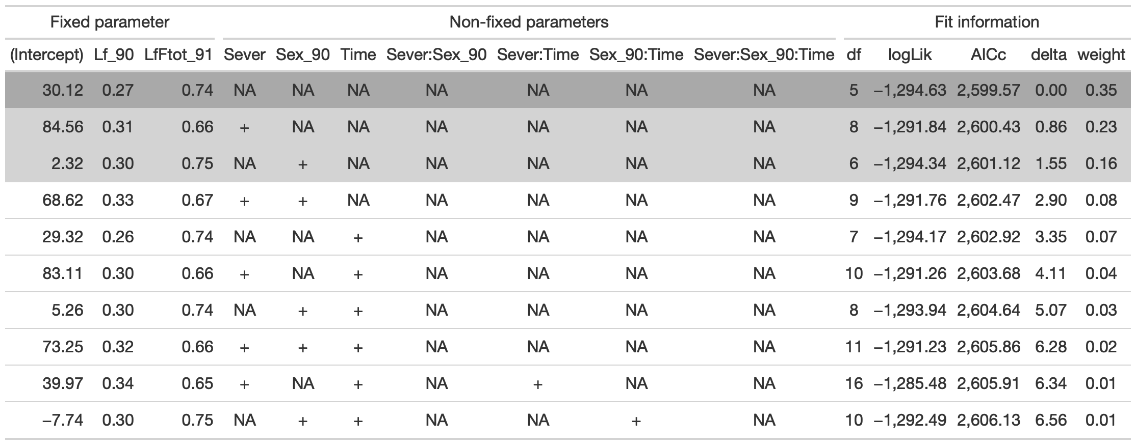  

The best model has fixed effects of Lf_90 and LfF_91.

6.2.3 Conclusion

d_mod92la.bm<-lmer(LftotF_92~+LfFtot_91+Lf_90+(1|COLONY), data = mayappleData, na.action ="na.fail")

The best model here contains fixed effects of leaf area in 1990 and 1991.

6.2.4 Estimated marginal means

the main effect of leaf area in 1990

mylist <- list(Lf_90=seq(150,1250,by=100))

g1 <- ggplot(data=mayappleData, aes(x=Lf_90, y=LftotF_92,color=Sever)) +
  geom_point(alpha=0.5) +
  ylab("Mean total leaf area \n in front shoots in 1992") 

g2 <- emmip(d_mod92la.bm,  ~ Lf_90 , at=mylist, CIs = TRUE)
gridExtra::grid.arrange(g1,g2,nrow=1)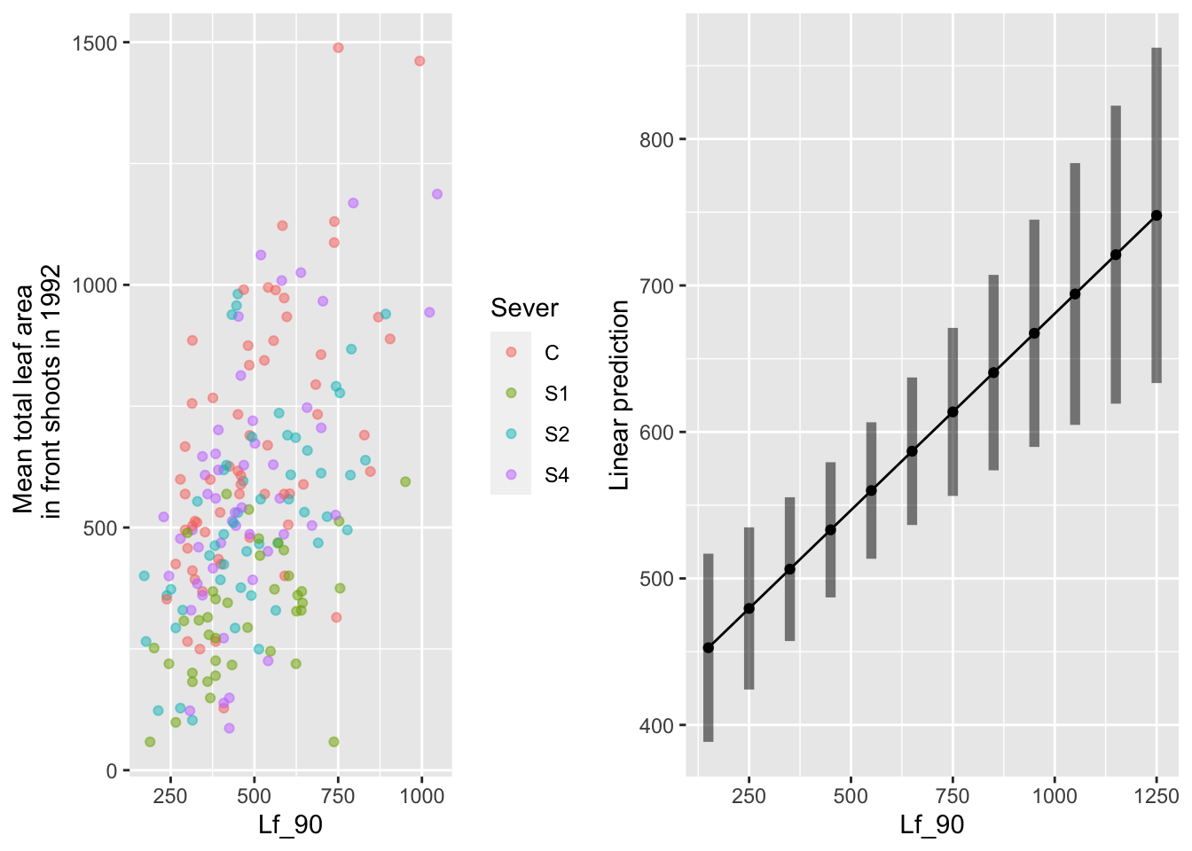

Of those systems that had non-zero leaf area in 1992, there is a positive relationship with leaf area in 1990.

the main effect of leaf area in 1991

mylist <- list(LfFtot_91=seq(0,1500,by=100))

g1 <- ggplot(data=mayappleData, aes(x=LfFtot_91, y=LftotF_92, color=Sever)) +
  geom_point(alpha=0.5) +
  ylab("Mean total leaf area \n in front shoots in 1992") 

g2 <- emmip(d_mod92la.bm,  ~ LfFtot_91 , at=mylist, CIs = TRUE)
gridExtra::grid.arrange(g1,g2,nrow=1)