Unit 10 GLPs

a GLP is a linear filter with a white noise input

We take white noise input and put it through a filter and get something that isnt white noise.

$$\sum_{j=0}^\infty \psi_j a_{t-j} = X_t - \mu$$

GLP’s are an infinite sum of white noise terms. This might be weird now but later on this concept will return.

The $\psi_j$’s are called psi weights, these will be useful again later. AR, MA, and ARMA are all special cases of GLP’s, and will be useful when we study confidence intervals.

10.1 AR(1) Intro

AR(p) in which p = 1

We will go through well known forms of the AR(1) model.

$$X_t = \beta + \phi_1 X_{t-1} + a_t$$

$$\beta = (1-\phi_1)\mu$$

Beta is moving average constant

We are saying that the vluse of x depends on some constant, the previous value of x, and some random white noise. Looks a lot like regression except there is a wierd variable

we can rewirte tis as

$$X_t = (1-\phi_1)\mu + \phi_1 X_{t-1} + a_t$$

An are 1 process is stationary iff the magnitude of $\phi_1$ is less than 1

We will deal with this a lot in the near future

10.1.1 AR(1) math zone

$$E\left[ X_t \right] = \mu ?$$ $$E \left[ X_t \right] =E \left[ 1-\phi_1 \mu \right] + E \left[ \phi_1 X_{t-1} \right] + E[a_t]$$

We can rewrite this as $$E \left[ X_t \right] = 1-\phi_1 \mu + \phi_1E \left[ X_{t} \right] + 0$$

$$E \left[ X_t \right] ( 1-\phi_1) = 1-\phi_1 \mu$$ $$E\left[ X_t \right] = \mu$$

Mean does not depend on T

The variance also does not, and if phi1 is less than one variance is finite

$$\sigma_X^2 = \frac{\sigma_a^2}{1-\phi_1^2}$$

and rhok is phi1 to the k

$$\rho_k = \phi_1^k, k \geq 0$$

Spectral Density of AR(1) also does not depend on time, it just monotonically increases or decreases depending on phi1:

$$S_X(f) = \frac{\sigma_a^2}{\sigma_X^2} \left( \frac{1}{\mid 1 - \phi_1 e^{-2\pi i f}\mid^2} \right)$$

10.1.2 the zero mean form of AR1

with zero mean, $$X_t = \phi_1 X_{t-1} + a_t$$ OR $$X_t- \phi_1 X_{t-1}$$ A

10.1.3 AR1 with positive phi

remember we have $$\rho_k = \phi_1^k$$

With positive $\phi_1$, we have:

realizations are wandering and aperiodic

Autocorrelations are damped exponentials

Spectral density Peaks at zero.

Higher values = stronger versions of these characterstics

10.1.4 AR1 with negative phi

We have:

realization are oscillating

Autocorrelations are damped and alternating(negative to a power you fool)

Spectral density* has a peak at f = 0.5 (cycle length of 2)

Higher magnitude = stronger characteristics

10.1.5 Nonstationary

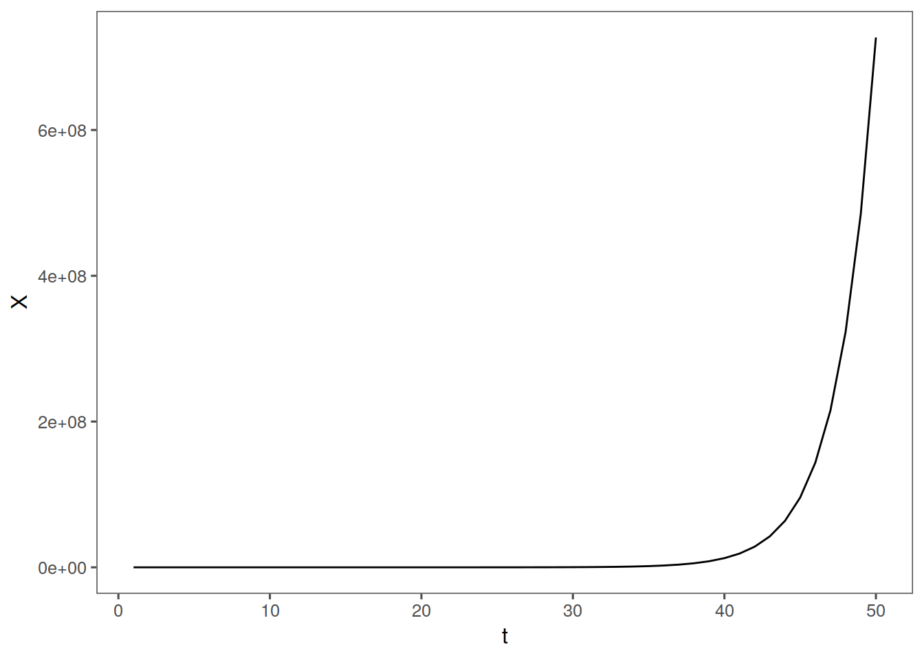
if phi = 1 or phi> 1, we have that realizations are from a nonstationary process. with it equal to one, it looks ok, and is actualy a special ARIMA model. WIth it > 1, we have crazy explosive realizations. Check this out:

nonstarma <- function(n, phi) {
    x <- rep(0, n)
    a <- rnorm(n)
    x[1:n] <- 0
    for (k in 2:n) {
        x[k] = phi * x[k - 1] + a[k]
    }
    tplot(x)
}

nonstarma(n = 50, phi = 1.5) + th