Unit 25 AR(p) forecast math

$$\hat{X}_{t_0} (\ell) = \phi_1 \hat{X}_{t_0}(\ell -1) + ... + \phi_p \hat{X}_{t_0}(\ell - p) + \bar{X} (1 - \phi_1 - ... - \phi_p))$$

25.1 AR(p) forecasts:

arpgen <- function(vec, l, mu, phi) {
    v <- vec[length(vec):(length(vec) - (length(phi) - 1))]
    f <- sum(phi * (v)) + mu * (1 - sum((phi)))
    if (l == 1) 
        return(f)
    return(arpgen(append(vec, f), l - 1, mu, phi))
    
}

arp <- function(vec, l, mu, phi) {
    as.numeric(lapply(1:l, arpgen, phi = phi, vec = vec, mu = mu))
}
x <- c(27.7, 23.4, 21.2, 21.1, 22.7)
p <- c(1.6, -0.8)
avg <- 29.4
arp(phi = p, vec = x, l = 5, mu = avg)

## [1] 25.32000 28.23200 30.79520 32.56672 33.35059

25.1.1 With tswge

25.1.1.1 positive phi, AR(1)

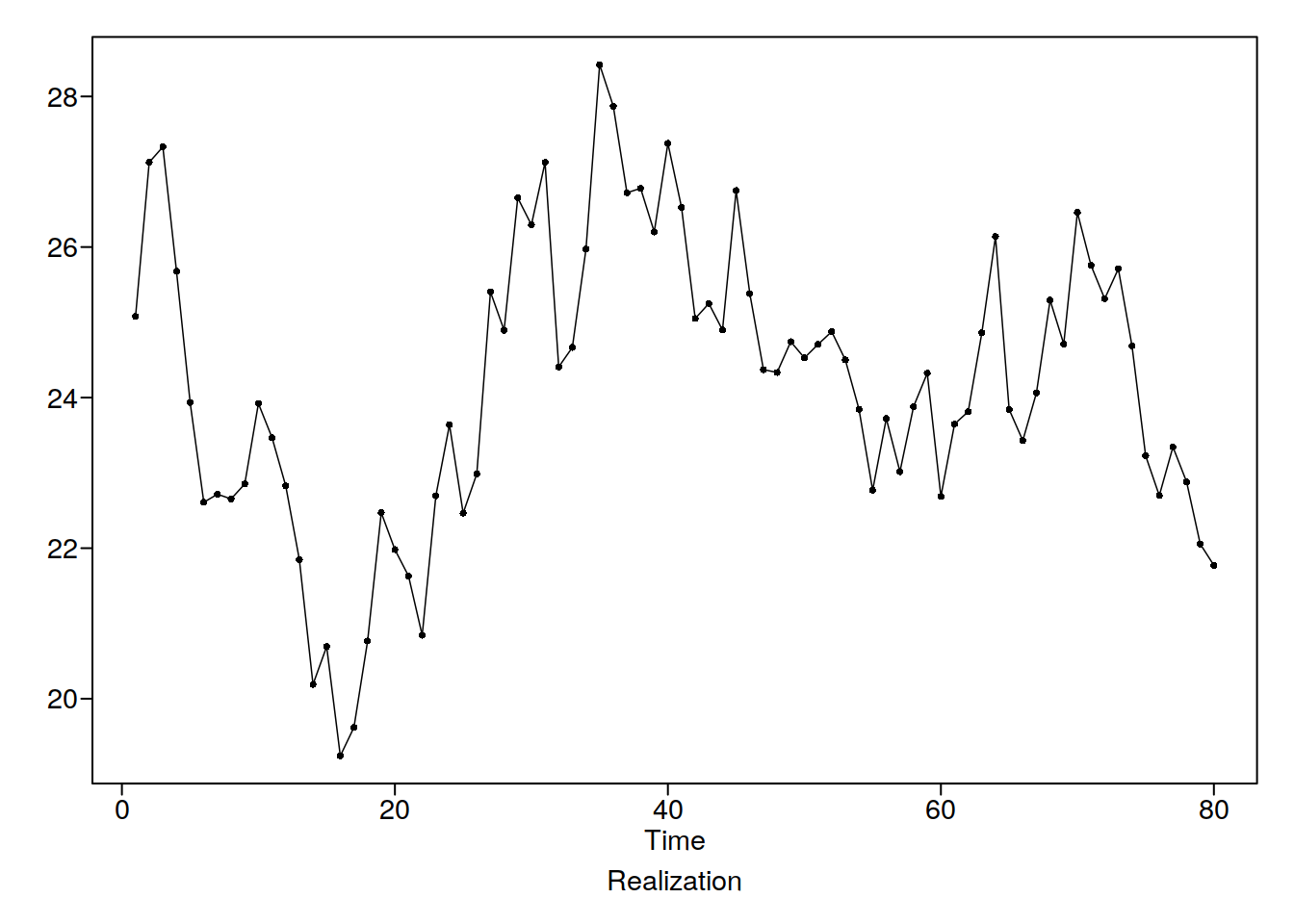
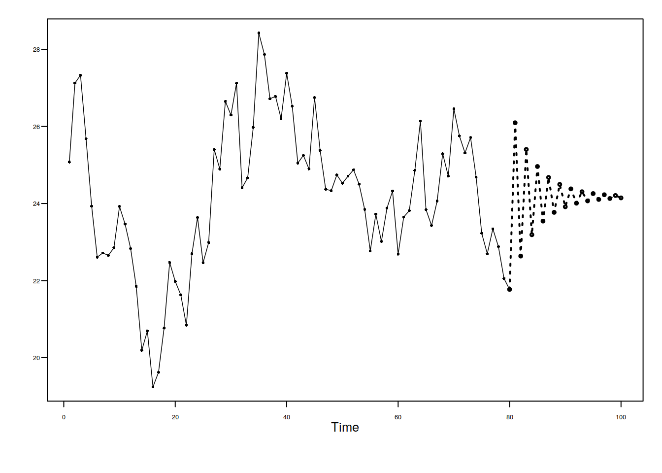
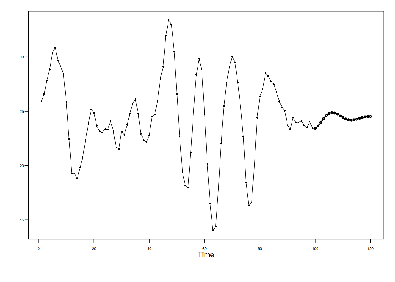
data(fig6.1nf)
plotts.wge(fig6.1nf)
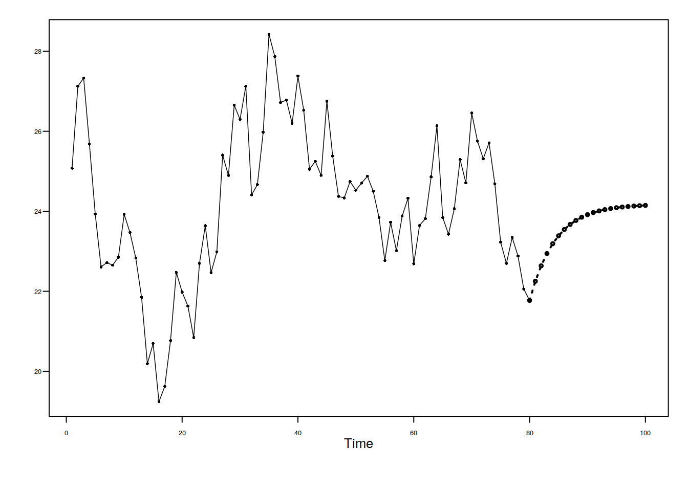
fore.arma.wge(fig6.1nf, phi = 0.8, n.ahead = 20, limits = F)

25.1.1.2 Negative phi, AR(1)

ts100 <- tswgen(100, sn = 24)
X1 <- ts100$sig(phi = -0.8)

fore.arma.wge(fig6.1nf, phi = -0.8, n.ahead = 20, limits = F)

It has the same behavior as the AR(functions). Sweet.

25.1.1.3 AR(2)

X2 <- ts100$sig(phi = c(1.6, -0.8))

X2 <- X2 + 25
plotts.wge(X2)

fore.arma.wge(X2, phi = c(1.6, -0.8), n.ahead = 20, limits = F)