Unit 5 Autocorrelation Concepts and Notation

5.1 Theoretical concept of $\rho$

$$\rho = \frac{E\left[\left(X-\mu_X\right)\left(Y-\mu_Y\right)\right]}{\sigma_X \sigma_Y} = \frac{\mathrm{covariance between X+y}}{\sigma_X \sigma_Y}$$

In a stationary time series, we have autocorrelation and autocovariance

5.2 autocovariance

$$\gamma_k = E\left[\left(X_t - \mu\right)\left(X_{t+k} - \mu\right)\right]$$

5.3 autocorrelation

$$\rho_k =\frac{E\left[\left(X_t - \mu\right)\left(X_{t+k} - \mu\right)\right]}{\sigma_{X_t} \sigma_{X_{t+k}}} = \frac{E\left[\left(X_t - \mu\right)\left(X_{t+k} - \mu\right)\right]}{\sigma^2_X} = \frac{\gamma_k}{\sigma_X^2}$$

This works because of constant variance and constant mean!

Note that in a stationary time series:

$$\sigma_X^2 = 1E[(X_t - \mu)^2] = E[(X_t -\mu )(X_t - \mu)] = \gamma_0$$

Therefore:

$$\rho_k = \frac{\gamma_k}{\gamma_0}$$

5.4 Stationary Covariance

Correlation is not affected by where, only by how far apart, that is: $$\rho_h = \mathrm{Cor} \left(X_t, X_{t+h}\right)$$

Let us try it out with this little snippet:

ggsplitacf <- function(vec) {
    h1 <- vec[1:(length(vec)/2)]
    h2 <- vec[(length(vec)/2):length(vec)]
    first <- ggacf(vec) + ggthemes::theme_few()
    second <- ggacf(h1) + ggthemes::theme_few()
    third <- ggacf(h2) + ggthemes::theme_few()
    cowplot::plot_grid(first, second, third, labels = c("original", "first half", 
        "second half"), nrow = 2, align = "v")
}

Realize = gen.arma.wge(500, 0.95, 0, sn = 784)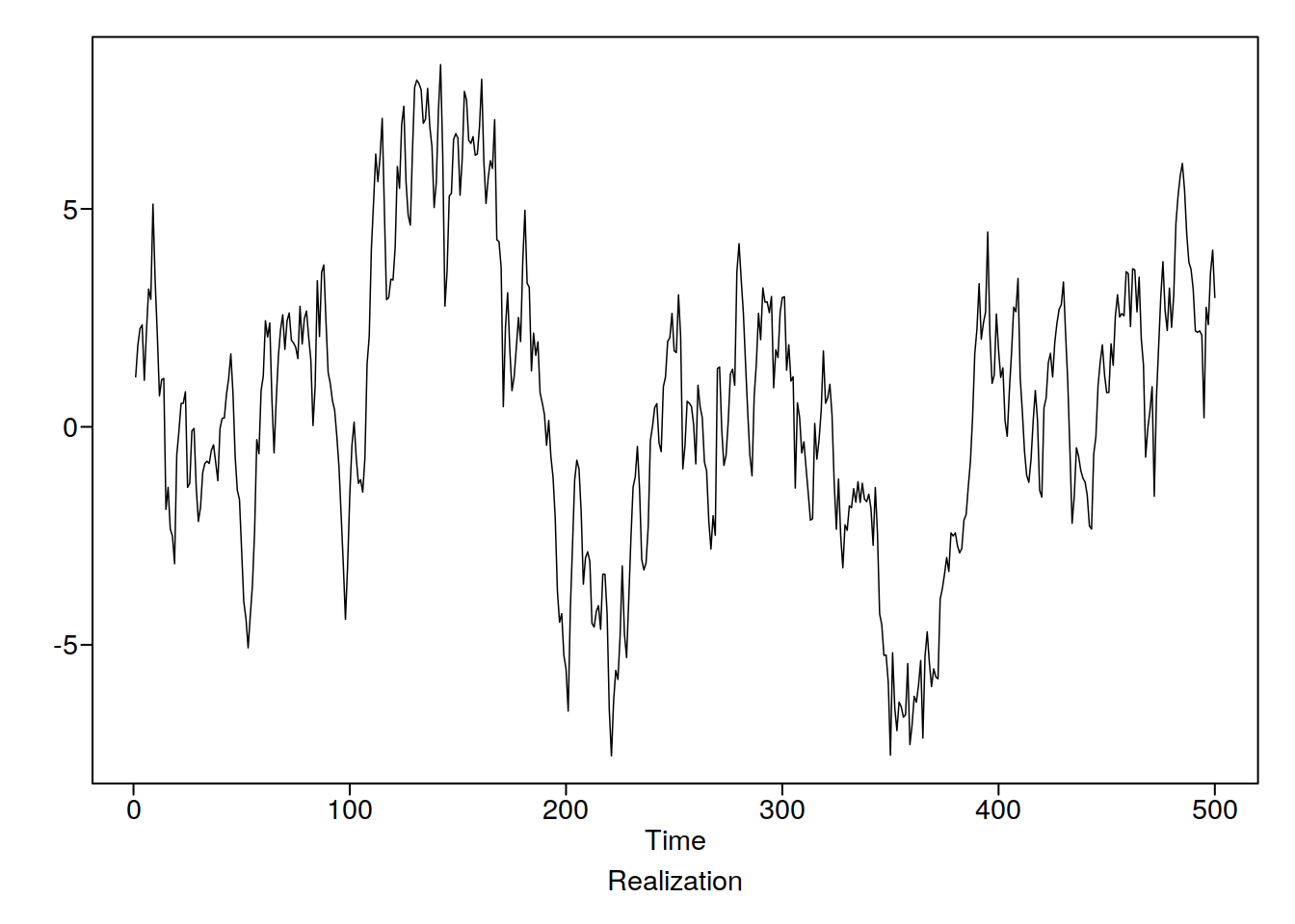

Lets check out the ACF

ggsplitacf(Realize)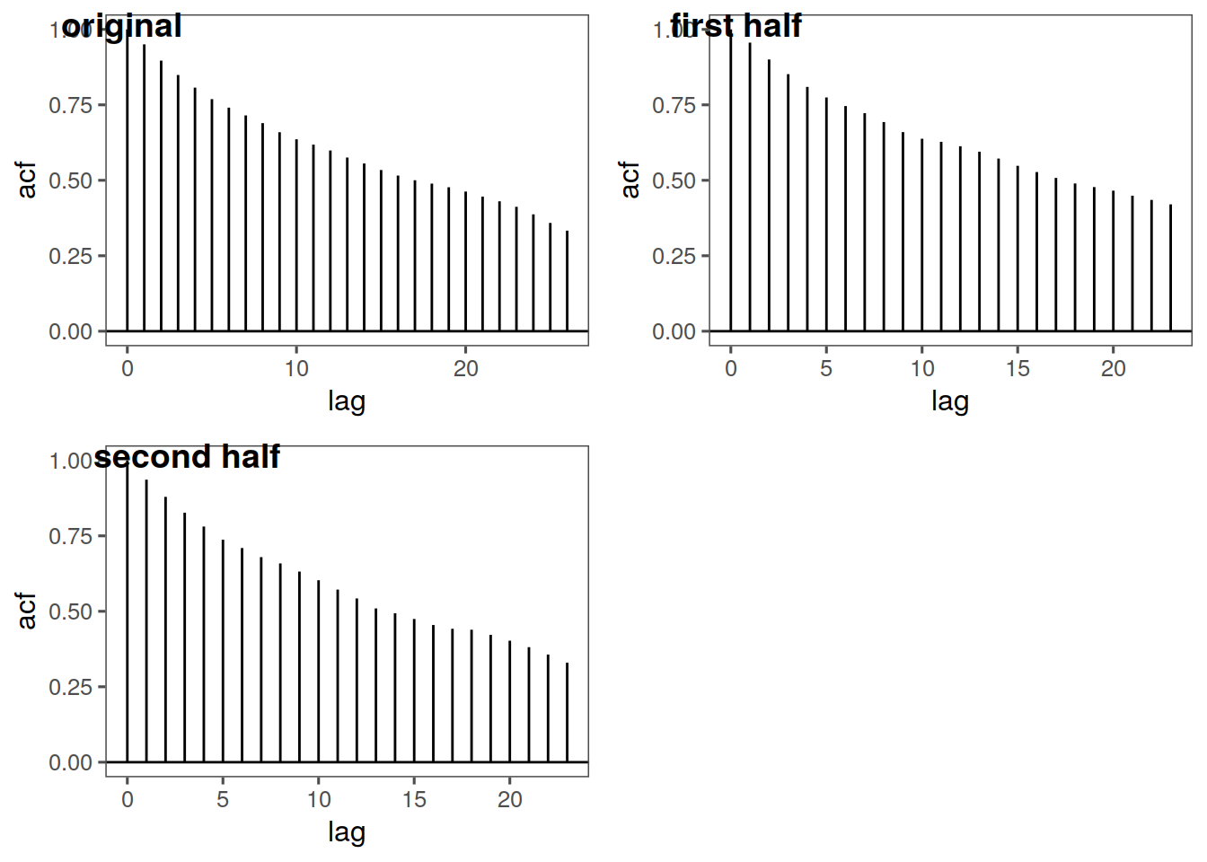

This looks pretty stationary to me! Let’s try with some sample data:

data("noctula")
tplot(noctula) + ggthemes::theme_few()
ggsplitacf(noctula)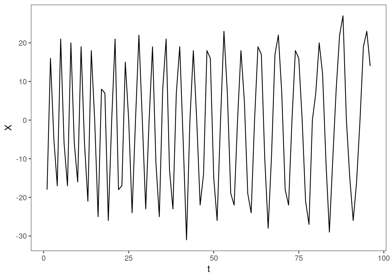

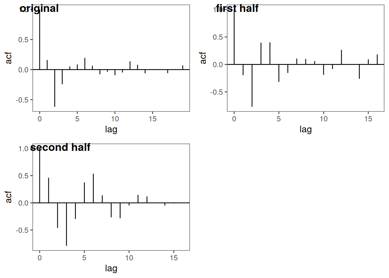
So in this case our mean probably looks constant, our variance could be constant as well, however the ACFs are clearly different. Let’s look at a different dataset:

data(lavon)
tplot(lavon) + ggthemes::theme_few()
ggsplitacf(lavon)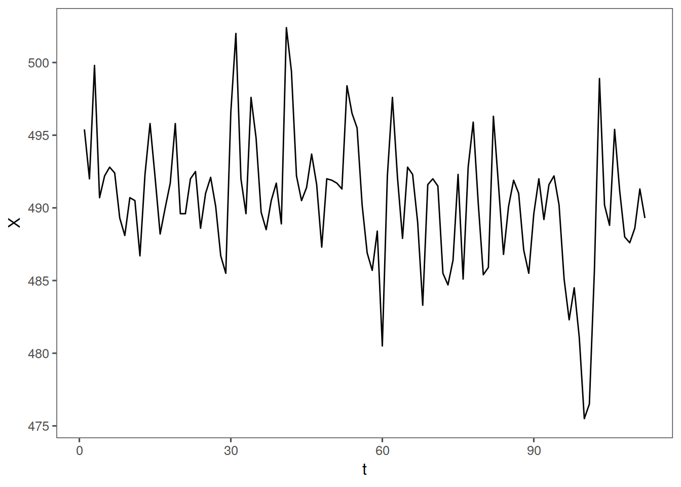

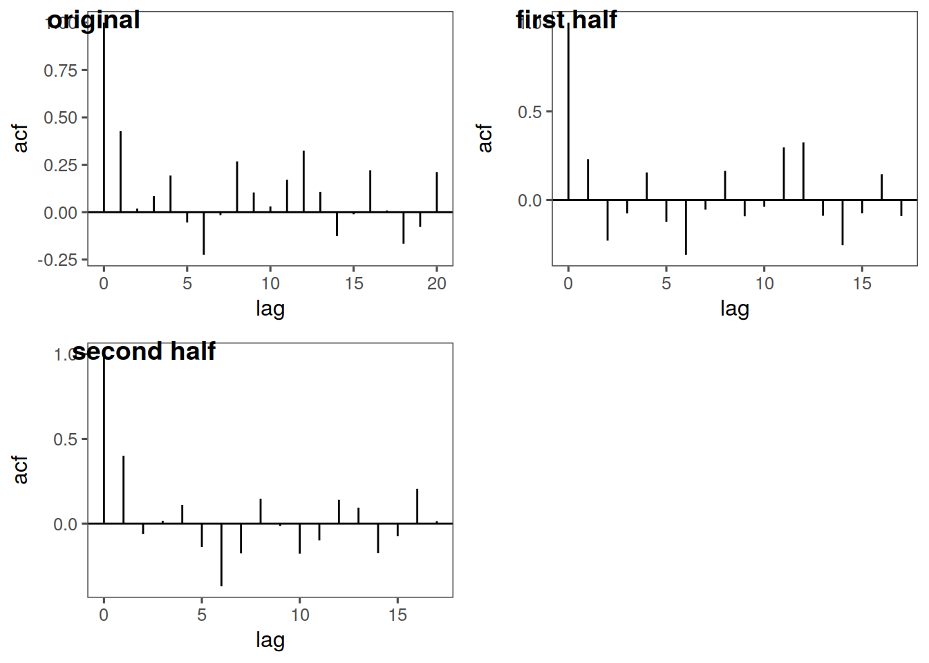
In this case, our mean looks maybe to be constant around 495, our variance does not appear to be constant, and our ACF looks pretty good, however I would say overall this probably is not stationary, due to the variance and slightly off ACF.