Unit 3 A Brief Discussion of Stationarity

In order for a time series to be considered stationary, it must satisfy three conditions:

• Constant Mean with Time

• Constant Variance with Time

• Constant Autocorellation with Time

3.1 Condition One: Constant Mean

Mean is constant with time. That is \(E[X_t] = \mu\). Note the lack of a little tiny t in mu! It is indepoent of tine! That is stationarity condition number 1!

Important result: If we assume constant mean, we can use all of the data to estimate the mean

Here we can see after 5 realizations that the mean is clearly not constant with time

library(tswge)
a1 = gen.sigplusnoise.wge(100, coef = c(5, 0), freq = c(0.1, 0), psi = c(3, 
    0), vara = 3, plot = F)
b1 = gen.sigplusnoise.wge(100, coef = c(5, 0), freq = c(0.1, 0), psi = c(3, 
    0), vara = 3, plot = F)
c1 = gen.sigplusnoise.wge(100, coef = c(5, 0), freq = c(0.1, 0), psi = c(3, 
    0), vara = 3, plot = F)
d1 = gen.sigplusnoise.wge(100, coef = c(5, 0), freq = c(0.1, 0), psi = c(3, 
    0), vara = 3, plot = F)
e1 = gen.sigplusnoise.wge(100, coef = c(5, 0), freq = c(0.1, 0), psi = c(3, 
    0), vara = 3, plot = F)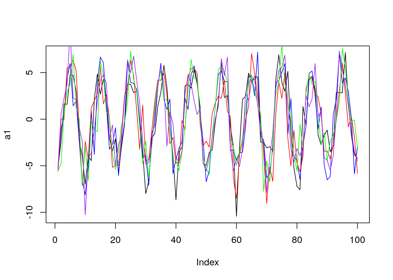

Now lets look at 5 realizations which come from the same realization, which might not have a constant mean:

a2 = gen.sigplusnoise.wge(100, coef = c(5, 0), freq = c(0.1, 0), psi = c(runif(1, 
    0, 2 * pi), 0), vara = 3, plot = F)
b2 = gen.sigplusnoise.wge(100, coef = c(5, 0), freq = c(0.1, 0), psi = c(runif(1, 
    0, 2 * pi), 0), vara = 3, plot = F)
c2 = gen.sigplusnoise.wge(100, coef = c(5, 0), freq = c(0.1, 0), psi = c(runif(1, 
    0, 2 * pi), 0), vara = 3, plot = F)
d2 = gen.sigplusnoise.wge(100, coef = c(5, 0), freq = c(0.1, 0), psi = c(runif(1, 
    0, 2 * pi), 0), vara = 3, plot = F)
e2 = gen.sigplusnoise.wge(100, coef = c(5, 0), freq = c(0.1, 0), psi = c(runif(1, 
    0, 2 * pi), 0), vara = 3, plot = F)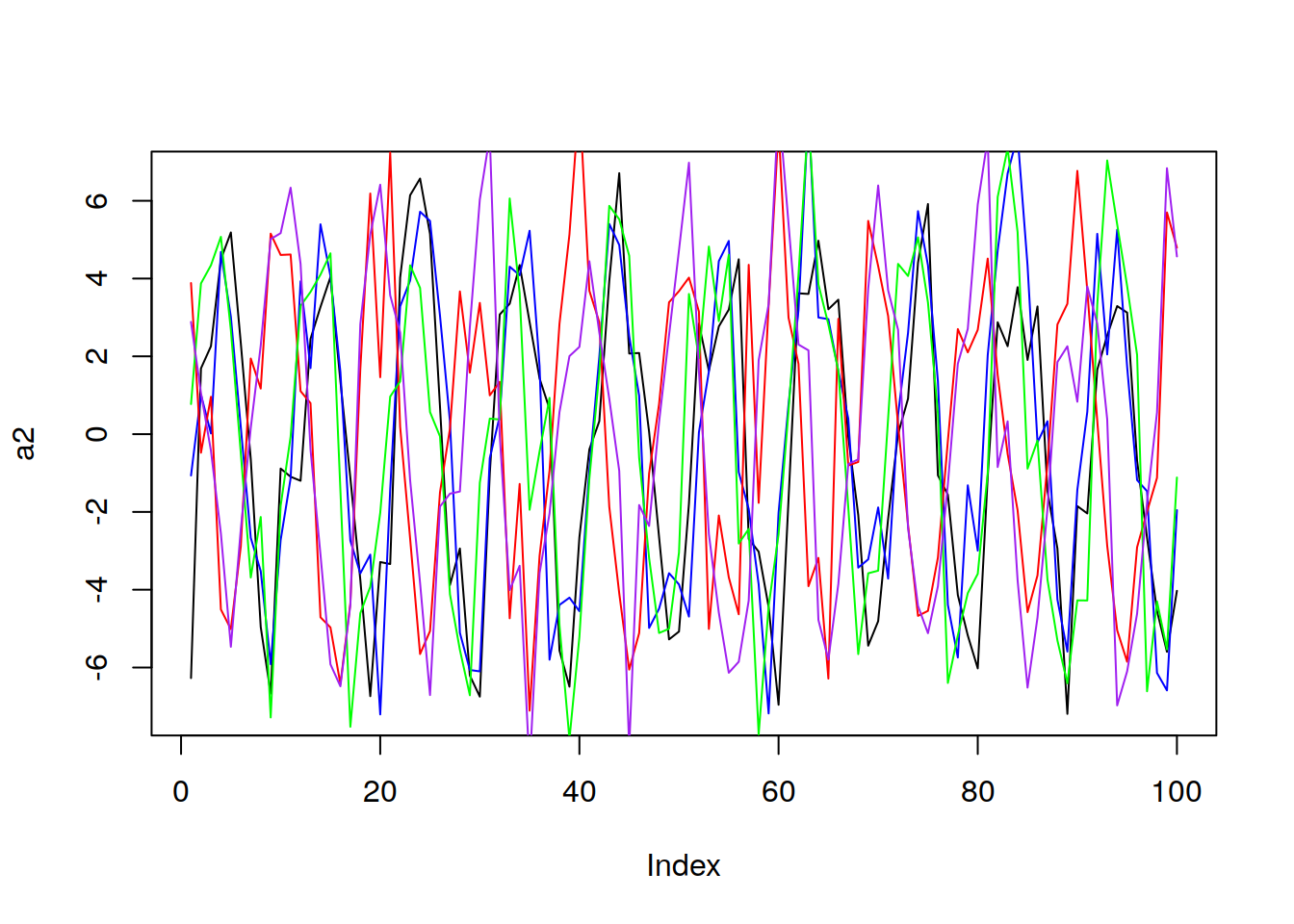

We cannot say for sure whether the mean is constant or not in this case!

3.2 Condition Two: Constant Variance

Variance does not depend on time

Variance is constant and finite*

That is :

\[Var[X_t] = \sigma^2 \neq \infty\]

If we can make this assumption, then we can use all of the data to make the variance. This is typically the hardest one to tell, and it will take some practice to see.

3.3 Condition 3: Constant autocorrelation

Correlation of \(X_{t_1} and X_{t_2}\) only depends on \(t_2 - t_1\)

That is, the correlation between points depends only on how far apart they are in time, not where they are in time.

To describe this mathematically:

Let \[h = t_2 - t_1\]

then \[\mathrm{Cor}\left(X_t,X_{t+h}\right) = \rho_h\]

\(\rho\) represents the population correlation coefficient.