Unit 20 ARIMA and ARUMA
Ok this is gonna be a light week, basically, in our notation, we have that ARIMA is an ARMA model with a wandering term, eg an equation with a root at exactly 1, and just one of them, while an ARUMA is a model where the backshift operator is squared. Mathematically we have:
20.1 ARIMA
\[(1 - B)^n X_t = a_t\] is an ARIMA (0,n,0) model. Note that because this is not stationary, we cannot view the plotts.true.wge :(
20.2 ARUMA
\[(1 - B^n) X_t = a_t \] is an ARUMA(0,n,0) model, or an ARIMA(0,0,0) model with a seasonal component of order n. This is pretty easy.
20.3 But what do they do????
ARIMA adds a wandering component, since the root is exactly one, while ARUMA is a seasonal model, because of sines and cosines and Euler’s theorem etc. Dont worry too much about it, try some stuff out with artrans.wge, gen.arima.wge, gen.aruma.wge etc. Here are some wrapper functions for artrans.wge:
20.3.1 ARIMA Transform
library(tswge)
arimatr <- function(xs, d) {
    f <- artrans.wge(xs, phi.tr = 1)
    if (d == 1) {
        f
    } else {
        arimatr(f, d - 1)
    }
}

x = gen.arima.wge(500, phi = c(0.6, -0.8), d = 2, theta = 0.3, sn = 35, plot = F)
d <- artrans.wge(x, phi.tr = 1)
d2 <- artrans.wge(d, phi.tr = 1)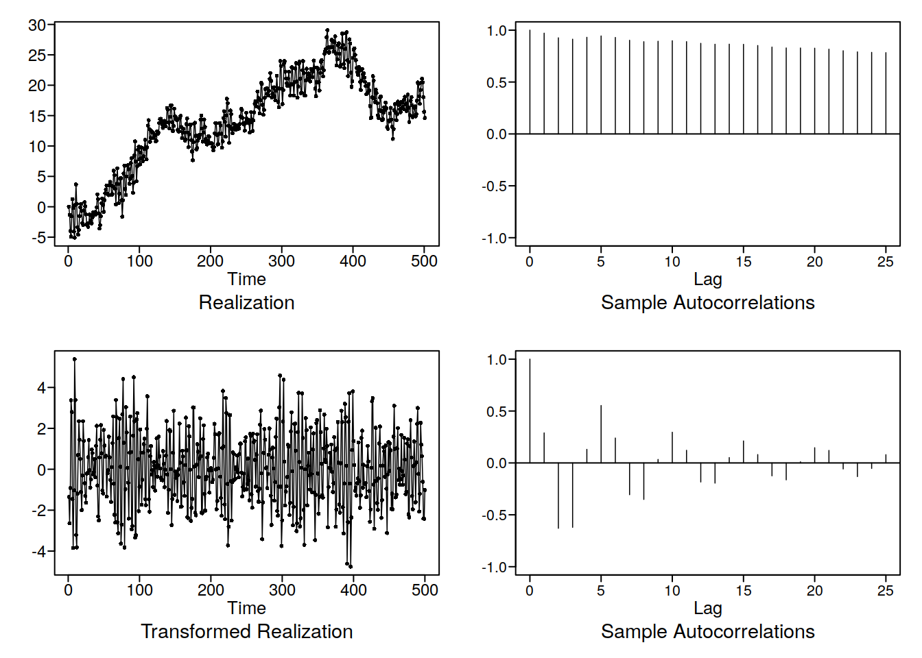
d3 <- arimatr(x, 2)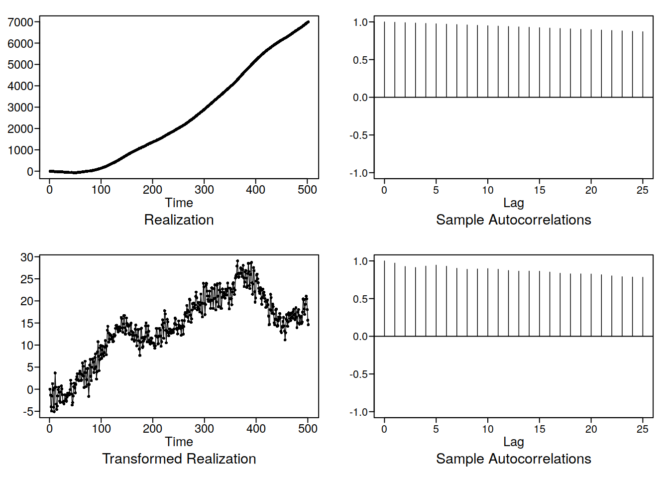

20.3.2 ARUMA Transform
arumatr <- function(xs, s) {
    artrans.wge(xs, phi.tr = c(rep(0, s - 1), 1))
}

x2 <- gen.aruma.wge(n = 200, s = 7, plot = F)
arumatr(x2, 7)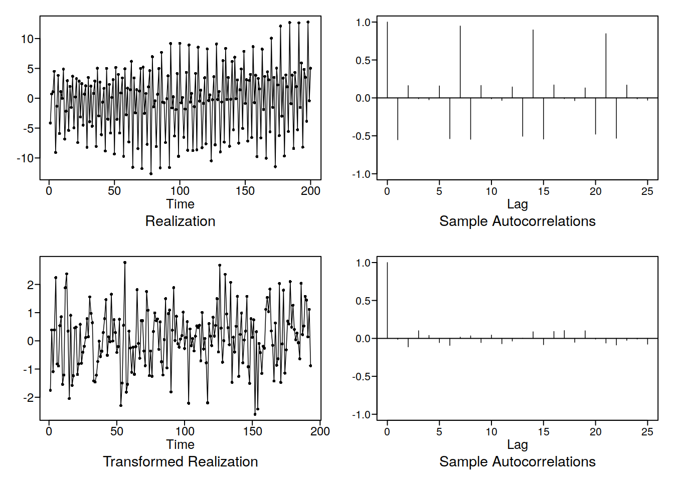
Again by transforming away the non stationary nonsense we end up with pure white noise in this case. We can check that with aic5.wge, it should be very confused